Semi-Analytical Solution Model for Bending Deformation of T-Shaped Aviation Aluminium Alloy Components under Residual Stress

Abstract

Structures composed of aviation aluminium alloys, characterized by their limited rigidity and thin-walled configurations, frequently exhibit deformation after processing. This paper presents an investigation into T-shaped components fabricated from pre-stretched 7075-T7451 aviation aluminium alloy sheets, examining the effects of residual stress and the geometrical parameters of T-shaped components on their deformational behavior. A semi-analytical model, developed to elucidate the bending deformation of T-shaped components subjected to residual stress, was validated through finite element analysis and empirical cutting experiments. The experimental results revealed that the bending deformation deflection of the T-shaped specimen was 0.920 mm, deviating by a mere 0.011 mm from the prediction provided by the semi-analytical model, resulting in an inconsequential error margin of 1.2%. This concordance underscores the precision and accuracy of the semi-analytical model specifically designed for T-shaped components. Moreover, the model’s simplicity and ease of application make it an effective tool for predicting the bending deformation of thin-walled T-shaped components under a range of residual stresses and dimensional variations, thereby demonstrating its significant utility in engineering applications.

1. Introduction

Aviation aluminium alloys, characterized by their lightweight properties and high specific strength, are extensively utilized in the aerospace sector [1]. Structures fabricated from aluminium alloy sheets, especially those of a thin-walled nature, are predominantly selected for aviation applications due to their capacity to enhance production efficiency, reduce product mass, shorten assembly durations, and decrease manufacturing expenses [2]. Nonetheless, these thin-walled aluminium alloy constructions routinely experience deformation post-manufacture. The accumulation of residual stress acts as a primary determinant of the extensive deformation observed in components, with the degree of deformation increasing in conjunction with residual stress levels [3]. The origin of residual stresses can be principally divided into two categories: initial residual stress (IRS) and machining-induced residual stress (MIRS) [4]. aluminium alloy plates, used as blanks for aerospace constructs, undergo complex fabrication processes that result in significant, heterogeneous residual stress fields within the material, termed initial residual stress. Furthermore, the mechanical machining process, especially cutting operations on thin-walled configurations which involve extensive material removal and lead to decreased rigidity of the component post-machining, generates cutting residual stress that further affects component deformation [5]. This type of residual stress is identified as machining-induced residual stress. Additionally, the likelihood of deformation in thin-walled components is intricately connected to the large dimensions of the component [6]. Aerospace structures, often elongated and capable of extending to several tens of meters in length, show reduced rigidity, making them prone to deformation following mechanical processing. Such deformation significantly impacts the precision of aerospace component fabrication, leading to increased production costs and reduced manufacturing efficiency [7].

Extensive investigations have been dedicated to elucidating the deformation mechanisms and developing predictive models for thin-walled structures. Weber et al. utilized the finite element method (FEM) to examine the effects of variable wall thicknesses, initial residual stresses, and machining-induced residual stresses on the deformation characteristics of integral thin-walled aluminium alloy double-frame components [8]. Using 2219 aluminium alloy thin-walled ring components as a case study, Li et al. developed a finite element simulation model based on ANSYS to analyze the deformation patterns during the machining of thin-walled components under various parameter conditions, concluding that residual stress within 2219 aluminium alloy ring components significantly affects the machining deformation of thin-walled structural components [9]. Yao et al., applying FEM techniques, assessed the impact of residual stress on the deformation of blade structural components and developed a deformation prediction model based on residual stress [10]. Wang et al., concentrating on 7075-T651(GB/T3880.2–2006) aluminium alloy three-frame thin-walled structural components, proposed an analytical model derived from elasticity theory to predict the effects of residual stress on deformation through different machining stages [11]. Jiang et al., analyzing multi-frame thin-walled structural components, investigated the effects of residual stress on deformation and established predictive models using software platforms such as ADVANTEDGE/DEFORM and ABAQUS [12]. Conducting finite element analysis, Li et al. modelled the layered milling of straight-face micro-thin-walled features with varying thicknesses to explore deformation patterns along the height and length of thin walls [13]. By adjusting the milling depth, Zheng et al. explored the machining deformation and stress distribution patterns under different cutting thicknesses, proposing a predictive model for machining deformation under varied milling conditions based on the theory of elastic deformation [14]. Zhu et al. considered both initial residual stresses and the operational loads on workpieces, creating a comprehensive model that includes equilibrium equations and stress boundary conditions through finite element methods to predict the resulting deformation in workpieces [15]. Ye developed a mechanical model for the machining deformation of 7075 aluminium alloy integral structural components using three-frame thin-walled structures and proposed a finite element model for analyzing the deformation of integral parts, demonstrating that simulation values closely align with calculated values with an error margin not exceeding 20% [16]. Integrating finite element analysis with empirical studies, Li et al. examined the impact of different material removal strategies and initial stress conditions on the deformation of aluminium alloy plates, noting the significant influence of asymmetric stress states on the deformation of thin plates [17]. Ju introduced a new analytical model based on the energy equation, incorporating the residual stress field informed by three-dimensional elasticity theory and the principle of minimum potential energy, using modified Rayleigh-Ritz and pseudoinverse methods to solve energy equations under various processing conditions for predicting the machining deformation of thin-walled ring components [18]. Gao et al., using 7075 aluminium alloy and Ti6Al4V titanium alloy as examples, investigated the effect of bending stiffness and residual stress on the dimensional stability of frame-like thin-walled workpieces through the finite element method [19].

Recently, interest has burgeoned in the investigation of the synergistic impact of initial and machining-induced residual stresses on the deformation behavior of components. Li et al. utilized the Bayesian network probabilistic graphical model as a framework to assess the uncertainties involved in the machining deformation of thin-walled entities. This exploration yielded an algorithmic approach to quantitatively elucidate the uncertainties associated with these factors, resulting in the development of a predictive deformation model [20]. Xue et al. focused their study on 2219 aluminium alloy’s thin-walled ring components, using both theoretical and finite element methods to analyze the spatial distribution of initial and machining-induced residual stresses, thereby revealing the deformational patterns under the influence of these stresses [21]. Zheng et al. investigated the effects of initial and machining-induced residual stresses on H-shaped thin-walled structural components, using finite element analysis [22]. Li et al., in their study, combined calculations of equivalent stiffness with plate and shell theory principles, proposing a predictive model that integrates both types of residual stress [23]. Li further advanced the discussion with a combined theoretical and numerical analysis of machining deformation mechanisms, establishing a springback model for tensile bending that incorporates the interplay of bending and machining-induced residual stresses, supported by a numerical model based on shell elements and submodel analysis techniques [24]. This approach highlighted that deformation trends are directly linked to the combined effects of cutting and bending residual stresses. Weber et al., considering the combined effects of initial and machining-induced residual stresses, advocated for a 3D linear elasticity finite element model. Applying this to frame-like structural components, they critically analyzed the impact of milling paths and wall thickness on the deformation of frame-like aluminium alloy thin-walled structures [25].

In summary, current research predominantly focuses on the deformation behavior and prediction for frame-like, plate-like, and ring-like thin-walled structures under the influence of residual stresses, with a notable lack of attention towards T-shaped configurations. Stemming from their origins in plate and beam designs due to superior load-bearing capabilities, T-shaped components are extensively utilized in various sectors, especially in aerospace and aviation, where they play crucial roles in aviation engine mounts and guide vanes, among others. This highlights the essential need for conducting deformation analysis and predictive modeling for T-shaped structures. Predominantly, current research methods rely on the FEM and the application of plate and shell theory. However, FEM requires specific computational hardware and software capabilities, along with extended computation times, while the use of plate and shell theory is hindered by its complex solving process, making both methods somewhat impractical for direct engineering applications. This study concentrates on T-section structural components made from 7075 aluminium alloy, noted for their reduced rigidity. It adopts an integrated methodological approach that combines theoretical analysis, finite element modeling, and empirical experimentation to enable the predictive study of deformation in these T-section structures. Moreover, this research introduces a semi-analytical model specifically designed to describe the bending deformation behaviors of T-section structural components when subjected to residual stresses.

2. Research Framework and Hypotheses

This study delineates an investigation into T-shaped structures fabricated from pre-stretched 7075-T7451 aviation aluminium alloy sheets manufactured by SOUTHWEST ALUMINIUM (GROUP) CO, LTD (Chongqing, China). The research is based on the following hypotheses [26]:

(1)

Internal residual stresses are assumed to be uniformly distributed at identical depths throughout the billet.

(2)

Residual stresses within the component are presumed to exist solely in the longitudinal and transverse directions, with any residual stresses in the thickness direction disregarded.

(3)

The study adheres to Kirchhoff’s hypothesis, which is applicable to the small deflection bending theory of thin plates. A thin plate is defined as having a thickness ($h$) less than one-fifth of its minimum characteristic dimension ($L$), symbolized as $h<L/5$. The small deflection bending of thin plates refers to instances where the plate’s maximum deflection ($w_{max}$) is less than one-fifth of its thickness ($h$), denoted as $w_{max}<h/5$.

(4)

Residual stresses are treated as internal forces. In addressing the bending deformation of components subjected to initial residual stresses, an equivalence principle of effect is employed, whereby initial residual stresses are analogously considered as external forces for analysis. Consequently, under this principle, deformations resulting from the release of residual stresses following material removal are equivalently analyzed as bending deformations induced by external forces. The methodology for this equivalence is detailed below.

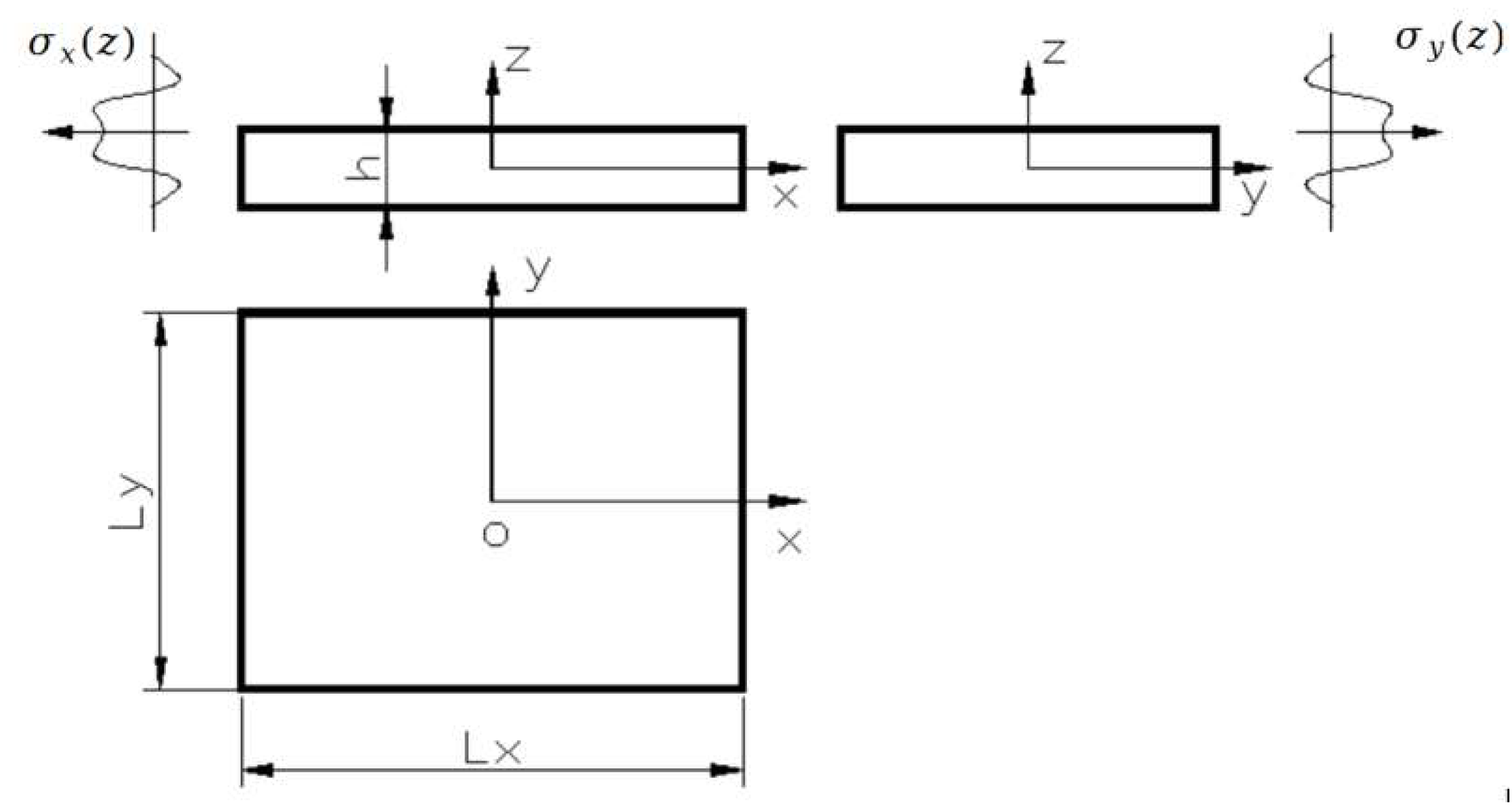
Assuming the post-processing model as shown in Figure 1, it is hypothesized that within the rectangular thin plate, there are initial residual stresses distributed along the thickness in the length direction ($L_x$) denoted as ${\sigma }_x\left(z\right)$, and in the width direction ($L_y$) denoted as ${\sigma }_y\left(z\right)$. Taking the central plane of the thin plate’s thickness as the reference plane, the bending moments $M_x$ and $M_y$, resulting from the stress components ${\sigma }_x$ and ${\sigma }_y$ acting on the central plane of the plate’s thickness, can be obtained using Equations (1) and (2).

$$M_x=\underset{-h/2}{\overset{h/2}{\int }}{\sigma }_x·z·dz$$

(1)

$$M_y=\underset{-h/2}{\overset{h/2}{\int }}{\sigma }_y·z·dz$$

(2)

$M_x$, $M_y$ are the uniformly distributed equivalent bending moments generated by the stresses ${\sigma }_x$, ${\sigma }_y$, respectively.

$M_x$ and $M_y$ can be calculated by Equations (1) and (2). The mechanical model of a rectangular thin plate with distributed moments on all four free edges is shown as Figure 2. Its bending deformation can be solved using plate and shell theory.

As shown in Figure 2, the geometric center of the rectangular plate is defined as the coordinate origin. When two sets of opposite edges are subjected to an equal reverse moments $M_x$ and $M_y$ respectively, the bending curvature can be expressed with the second derivative of the deflection function, bending moment, bending stiffness D, Poisson’s ratio μ, and modulus of elasticity E.

$$\frac{{\partial }^{2}w(x,y)}{\partial x^2}=\frac{M_x-\mu M_y}{D(1-{\mu }^2)}$$

(3)

$$\frac{{\partial }^{2}w(x,y)}{\partial y^2}=\frac{M_y-\mu M_x}{D(1-{\mu }^2)}$$

(4)

$$D=\frac{E{h}^3}{12(1-{\mu }^2)}$$

(5)

Here, $w(x,y)$ represents the deflection function which is expressed as Equation (6).

$$w(x,y)=\frac{M_x-\mu M_y}{2D(1-{\mu }^2)}{x}^2+\frac{M_y-\mu M_x}{2D(1-{\mu }^2)}{y}^2+C_{1}x+C_{2}y+C_3$$

(6)

When the tangent plane of the bent midplane at the origin is selected as the base plane of the variable $w$, $C_1$ = $C_2$ = $C_3$ = 0. Equation (6) can be transformed to Equation (7):

$$w(x,y)=\frac{M_x-\mu M_y}{2D(1-{\mu }^2)}{x}^2+\frac{M_y-\mu M_x}{2D(1-{\mu }^2)}{y}^2$$

(7)

When $M_y={\mu M}_x$, Equation (7) can be transformed to Equation (8). It can be seen from Equation (8) that the midplane is bent into a cylindrical surface, and it’s generatrix is parallel to the axis $y$.

$$w=\frac{M_x}{2D}{x}^2$$

(8)

Through the equivalence method, the equivalent stress situation of the T-shaped component is depicted in Figure 3. It is quite difficult to solve the deformation problem using plate and shell theory for the T-shaped component. A characteristic feature of T-shaped component is the presence of a central stiffener with significant height, which offers high bending resistance. However, while the web plate of a T-shaped component is notably thin and positioned far from the central stiffener, it is prone to early buckling before the entire component does. This observation has prompted the proposal of a novel method for analyzing the bending deformation of T-shaped components, dividing the analysis into separate evaluations for the bending deformations of T-beams and plates. Thus, the method for analyzing the bending deformation of T-shaped sections under residual stress, as shown in Figure 3, involves a separated approach, including the deformation analyses of both T-beams and rectangular cantilever plates. The sum of these individual deformations equates to the total bending deformation of the T-shaped component, as illustrated in Equation (9).

$$w=w_T+w_C$$

(9)

In Equation (9), $w_T$ represents the bending deformation of the T-beam, which can be calculated using well-established bending equations from mechanics of materials, as specified in Equation (10).

$$w_T=\frac{M_e·l^2}{2·E·I}$$

(10)

$M_e$ stands for the applied moment, $l$ indicates the length of the beam, $E$ is the elastic modulus, and $I$ denotes the moment of inertia relevant to the T-section.

In Equation (9), $w_c$ signifies the deformation of the rectangular web plate of the T-section component.

Cantilever thin plate is an important structural element while its bending has been one of the most difficult problems in the theory of elastic thin plate for the complexity in both the governing equation and the boundary conditions. The bending of rectangular thin plates with various combinations of boundary conditions has been investigated for many years by different authors [27]. However, the existing solutions are relatively complex and not convenient for engineering application. Therefore, a solution model for bending deformation of rectangular cantilever thin plates with simple calculation, convenience, and high accuracy, is the primary focus of this study.

3. Solution for Bending Deformation of Rectangular Cantilever Plates

When the central rib of a T-shaped structural component possesses significant height, its web can be viewed as a cantilever plate. This configuration’s load model is illustrated in Figure 4, where one side is fixed, and the remaining three sides are subjected to uniformly distributed moments $M_x$ and $M_y$. In this context, $M_x$ acts on the free edge, while $M_y$ is exerted on the edges parallel to the axis, with $M_y$ appearing in pairs. It is established that when $M_x$ and $M_y$ induce a concave deformation at the center of the plate, $M_x$ and $M_y$ are deemed positive, and conversely, negative when the effect is opposite. Utilizing this model, the controlled variable method is applied, with the finite element software ABAQUS (the version used in the study is 6.14-2) used to investigate the impact of cantilever length $L$, plate width $W$, plate thickness $t$, the ratio of cantilever length to plate width ($W/L$), and the magnitudes and ratio of $M_x$ to $M_y$ on the bending deformation of the cantilever plate, thereby deriving a solution model for the bending deformation of the cantilever plate.

3.1. Effect of Moment Magnitude on Cantilever Plate Deformation

3.1.1. Effect of $M_y$ Value on Rectangular Cantilever Thin Plate Bending Deformation

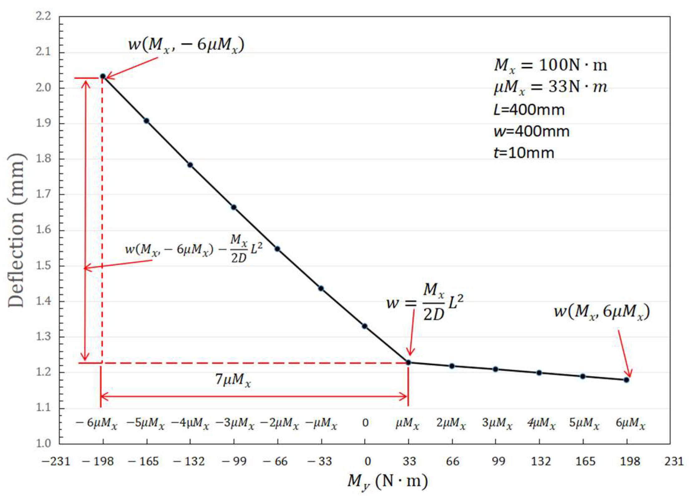
Using pre-stretched 7075-T7451 plate material, the dimensions of the cantilever thin plate are set to $L=W=400 \mathrm{mm}, t=10 \mathrm{mm}$. Bending deformation finite element simulations are conducted using the ABAQUS finite element software. The finite element model is established as shown in Figure 5, employing eight-node hexahedral linear non-conforming elements, with an element size of 2.5 mm × 2.5 mm × 1 mm (the billet is divided into ten layers along the thickness direction, each layer being 1 mm thick), totaling 256,000 elements. Other parameters are as shown in

Table 1. Parameters of finite element model.

Parameter Name	Parameter Values
Unit type	Eight node hexahedral linear non conforming mode
Unit size	2.5 mm × 2.5 mm × 1 mm
Number of units	256,000
Material density	2850 kg/m3
Elastic modulus	70.3 GPa
Poisson’s ratio	0.33
Yield limit	455 MPa

. To ensure that the thin plate belongs to the problem of small deflection bending (the deflection of the plate is less than 1/5 of the plate thickness), the applied load should be with in a certain range. For ease of comparative analysis, the applied load $M_x$ is set to whole values in $100 \mathrm{N}·\mathrm{m}$, with $M_y$ as a variable, tentatively taking thirteen different values for simulation analyses. The $M_y$ values are set as integer multiples of $\mu M_x$ (here $\mu$ is the Poisson’s ratio), with the values being: −198, −165, −132, −99, −66, −33, 0, 33, 66, 99, 132, 165, 198 $\mathrm{N}·\mathrm{m}$. Note that these moments are per unit length moments, considered as uniformly distributed moments. When applying them as concentrated moments in finite element analysis, the acting length must be multiplied. Post-simulation, the maximum deflection values of the cantilever thin plate are as shown in

Table 2. Deflection values of cantilever plate under different $M_y$ values.

Test Code	1	2	3	4	5	6	7	8	9	10	11	12	13
Mx ($\mathrm{N}·\mathrm{m}$)	100	100	100	100	100	100	100	100	100	100	100	100	100
My ($\mathrm{N}·\mathrm{m}$)	−198	−165	−132	−99	−66	−33	0	33	66	99	132	165	198
Deflection $w$ (mm)	2.032	1.907	1.783	1.664	1.547	1.436	1.330	1.228	1.218	1.209	1.199	1.189	1.179

. Since the deflection value of the rectangular cantilever plate reaches 1/5 of the plate thickness when value of $M_y$ is 198 $\mathrm{N}·\mathrm{m}$, 198 $\mathrm{N}·\mathrm{m}$ is determined as the maximum value of $M_y$ here.

To analyze the trend of deflection values of rectangular cantilever thin plates as a function of $M_y$ values, the data from Table 2 is represented graphically in Figure 6. It can be observed that the curve of deflection values approximates two intersecting straight lines with different slopes, intersecting at the applied moments of $M_x=100 \mathrm{N}·\mathrm{m}$ and $M_y=33 \mathrm{N}·\mathrm{m}$. When $M_y>33$ (i.e., $\mu M_x$), the deflection values $w$ approximately decrease linearly with an increase in $M_y$, showing minimal variation. Conversely, when $M_y<33$ (i.e., $\mu M_x$), the deflection values $w$ approximately increase linearly as $M_y$ increases negatively. Moreover, moments are applied as shown in Figure 4 and when $M_y=\mu M_x$, the cantilever thin plate bends in a cylindrical form, with the generatrices of the cylinder parallel to the Y-axis, as shown in Figure 7. The deflection value under these conditions can be determined with Equation (8) to obtain an analytical solution. The result calculated from Equation (8) is 1.217 mm, consistent with the simulation results (with an error of only 1%).

3.1.2. Effect of Linear Variation of Moments on the Bending Deformation of Rectangular Cantilever Plates

To analyze the influence of variations in moments $M_x$ and $M_y$ on deflection values, data from Table 1 was utilized as a basis to investigate the trend of deflection changes with proportional variations in $M_x$ and $M_y$. The $M_x$ and $M_y$ in

Table 3. Deflection values of cantilever plate bending deformation when moments are reduced by half.

Test Code	1	2	3	4	5	6	7	8	9	10	11	12	13
Mx ($\mathrm{N}·\mathrm{m}$)	50	50	50	50	50	50	50	50	50	50	50	50	50
My ($\mathrm{N}·\mathrm{m}$)	−99	−82.5	−66	−49.5	−33	−16.5	0	16.5	33	49.5	66	82.5	99
Deflection $w$ (mm)	1.016	0.953	0.892	0.832	0.774	0.716	0.665	0.614	0.609	0.604	0.599	0.595	0.59

are half those of the corresponding $M_x$ and $M_y$ in Table 1, as determined using finite element software to obtain the deflection values of the cantilever thin plate, as shown in Table 1. It was observed that the deflection values decreased by half compared to the values in Table 1. Through multiple analyses, it has been understood that, within the yield limit, when the applied moments $M_x$ and $M_y$ are varied linearly, the deflection values also exhibit a linear change in the same direction.

As demonstrated in Figure 6, after determining the deflection value at the intersection point using Equation (8), the deflection values under any moment can be ascertained by simply calculating the slopes of these two curves. To enhance calculation precision, the endpoints of the two lines in Figure 6 can be considered, namely, at $M_y=6\mu M_x$ and $M_y=-6\mu M_x$. The deflection value of the two endpoints are denoted as $w(M_x,-6\mu M_x)$ and $w(M_x,6\mu M_x)$. The slope of the two lines in Figure 6 can be expressed as $\left[w(M_x,-6\mu M_x)-\frac{M_x}{2D}·L^2\right]/(-6\mu M_x-\mu M_x)$ and $\left[w(M_x,6\mu M_x)-\frac{M_x}{2D}·L^2\right]/(6\mu M_x-\mu M_x)$ respectively. The deflection values under any moment can subsequently be calculated using Equations (11) and (12).

For $M_y\le \mu M_x$, it is derived as Equation (11).

$$w=\frac{w·(M_x,-6\mu M_x)-\frac{M_x}{2·D}·L^2}{-7\mu M_x}\times (M_y-\mu M_x)+\frac{M_x}{2D}·L^2$$

(11)

For $M_y>\mu M_x$, it is formulated as Equation (12).

$$w=\frac{w·(M_x, 6\mu M_x)-\frac{M_x}{2·D}·L^2}{5\mu M_x}\times (M_y-\mu M_x)+\frac{M_x}{2·D}·L^2$$

(12)

Here, $M_x$, $M_y$ are the uniformly distributed equivalent bending moments loaded on the four free edges as shown in Figure 4, D is bending stiffness, $D=\frac{E{·t}^3}{12(1-{\mu }^2)}$, μ is Poisson’s ratio, E is modulus of elasticity, L is the length of the cantilever plate, and t is the thickness of the cantilever plate.

Deflection w in Table 2 are also calculated according to Equations (11) and (12). The maximum error between the calculation results and the simulation results is only 1.65%, which reveals that formula Equations (11) and (12) are reliable.

Although the forms of Equations (11) and (12) are simple, it was impossible to obtain the maximum deflection value of a rectangular cantilever thin plate with the two equations. The boundary conditions of the free edges of the cantilever plate are asymmetric, which results in complex analytical solutions for the deflection values ($w(M_x,-6\mu M_x)$ and $w(M_x,-6\mu M_x)$) at both endpoints of the straight line. How to obtain the value of $w(M_x,-6\mu M_x)$ and $w(M_x,-6\mu M_x)$ has become the key to deflection values under any moment. Given that the finite element method can handle such complex boundary conditions and provide stable numerical solutions, the finite element method is employed to obtain the deflection value at these endpoints.

However, the finite element analysis method has limitations and computational complexity, such as its results being affected by the accuracy and type of mesh division. A mesh type that is too rough may not capture the details of the structure, leading to inaccurate results, while a mesh type that is too fine usually requires a large amount of computing resources, such as memory and processor resources, which result in high computational costs and long time. Therefore, when the finite element method is applied to obtain the solution of $w(M_x,-6\mu M_x)$ and $w(M_x,6\mu M_x)$, we pay more attention to analyze the influencing factors of $w(M_x,-6\mu M_x)$ and $w(M_x,6\mu M_x)$, and the influence laws, in order to obtain a simple, convenient, and universal mathematical solution model.

3.2. Effect of Cantilever Dimensions on Deformation

3.2.1. Effect of Plate Dimension Ratio ($W/L$) on Cantilever Plate Bending Deformation

Equations (11) and (12) can be utilized to calculate the deflection values of a cantilever plate with dimensions 400 mm × 400 mm × 10 mm under any applied moments. The applicability of these equations when the width of the plate varies is a question that warrants investigation. Accordingly, this paper analyzes the pattern of deformation of cantilever plates as the $W/L$ ratio changes.

A constant cantilever length of $L=400 \mathrm{m}\mathrm{m}$ and thickness of $t=10 \mathrm{m}\mathrm{m}$ were selected. The width $W$ was varied across nine series: 80 mm, 100 mm, 200 mm, 300 mm, 400 mm, 500 mm, 600 mm, 700 mm, and 800 mm, resulting in nine plates in total. Each plate was subjected to the moments listed in Table 1 for simulation analysis, yielding the deflection values as shown in

Table 4. Deflection Values of Cantilever Plates with Different Width Dimensions.

Test Code	1	2	3	4	5	6	7	8	9	10	11	12	13
Mx ($\mathrm{N}·\mathrm{m}$)	100	100	100	100	100	100	100	100	100	100	100	100	100
My ($\mathrm{N}·\mathrm{m}$)	−198	−165	−132	−99	−66	−33	0	33	66	99	132	165	198
$w_{80}$ (mm)	2.159	2.030	1.896	1.762	1.628	1.495	1.361	1.228	1.100	0.972	0.843	0.715	0.587
$w_{100}$ (mm)	2.135	2.005	1.875	1.745	1.616	1.486	1.357	1.228	1.107	0.986	0.864	0.743	0.621
$w_{200}$ (mm)	2.043	1.924	1.806	1.687	1.570	1.456	1.341	1.228	1.144	1.059	0.974	0.890	0.805
$w_{300}$ (mm)	2.020	1.901	1.783	1.667	1.553	1.442	1.334	1.228	1.182	1.136	1.089	1.043	0.997
$w_{400}$ (mm)	2.032	1.907	1.783	1.664	1.547	1.436	1.330	1.228	1.218	1.209	1.199	1.189	1.179
$w_{500}$ (mm)	2.050	1.918	1.788	1.664	1.544	1.431	1.327	1.228	1.250	1.271	1.293	1.315	1.336

. To depict the pattern of change, the data from Table 4 is graphically represented in Figure 8. It is observed that for each specification of the plate, the variation pattern of deflection under applied moments is consistent with that shown in Figure 6, characterized by two intersecting lines of different slopes at the 8th point (applied moments: $M_x=100 \mathrm{N}·\mathrm{m}, M_y=\mu M_x=33 \mathrm{N}·\mathrm{m}$). The only difference is the slope of the lines, which varies with the plate dimension. The $W/L$ ratio change results in the change of its bending stiffness D, which cause different slopes of straight lines. From Table 4, it can be seen that when W, the width of the plate changes linearly, the deflection of the plates does not show a linear change pattern, though the plates are subjected the moments of the same magnitude. This can also be seen from the non-uniform changes of the slopes of each straight line in Figure 8. It can be concluded that the bending stiffness of a rectangular cantilever thin plate is not linearly related to the variation of its dimension. The nonlinear change poses difficulties in solving the problem. It is also noted that irrespective of the changes in plate $W/L$ ratio, as long as the condition $M_y=\mu M_x$ is met, Equation (8) can be used to obtain an analytical solution for the bending deformation of the cantilever plate under such moments. As long as the deflection values $w(M_x,-6\mu M_x)$ and $w(M_x,6\mu M_x)$ at the endpoints of the straight line are obtained, the deflection values of these cantilever plates can be calculated with Equations (11) and (12).

The challenge in calculating deflection values using Equations (11) and (12) arise from the determination of the slopes in Figure 7. This challenge can be transformed into the problem of calculating the deflection values at the endpoints of the two lines, specifically at $M_y=-6\mu M_x$ and $M_y=6\mu M_x$, denoted as $w·(M_x,-6\mu M_x)$, $w·(M_x, 6\mu M_x)$. These deflection values must be obtained through finite element analysis for each instance. Identifying a pattern in the variation of these deflection values with changes in plate dimensions would resolve the issue of computing the deflection for a cantilever plate with a length of 400 mm and a thickness of 10 mm.

To discern the pattern of change in the deflection values at the endpoints of the lines depicted in Figure 8 with varying plate dimensions, 23 cantilever plates were selected. These plates have a constant length of $L=400 \mathrm{m}\mathrm{m}$, a thickness of $t=10 \mathrm{m}\mathrm{m}$, and its $W/L$ ratio is selected in the range of $0.1\le W/L\le 10$ according to the actual engineering applications. Considering the uniformity of distribution, the specific width is determined as 40 mm, 60 mm, 80 mm, 100 mm, 200 mm, 300 mm, 400 mm, 500 mm, 600 mm, 700 mm, 800 mm, 900 mm, 1000 mm, 1200 mm, 1400 mm, 1600 mm, 1800 mm, 2000 mm, 2400 mm, 2800 mm, 3200 mm, 3600 mm, 4000 mm.

After applying torques of $M_x=100 \mathrm{N}·\mathrm{m}$ and $M_y=198 \mathrm{N}·\mathrm{m}$, as well as $M_x=100 \mathrm{N}·\mathrm{m}$ and $M_y=-198 \mathrm{N}·\mathrm{m}$, to these 23 groups of cantilever plates, the simulation results for deflection values are shown in

Table 5. Deflection values under different plate dimension ratios.

x (W/L)	0.1	0.15	0.2	0.25	0.5	0.75	1	1.25
f1(x) (mm)	2.230	2.195	2.159	2.136	2.043	2.02	2.032	2.050
f2(x) (mm)	0.52	0.552	0.586	0.621	0.805	0.997	1.179	1.336
x (W/L)	1.5	1.75	2	2.25	2.5	3	3.5	4
f1(x) (mm)	2.050	2.048	2.022	1.984	1.938	1.839	1.774	1.743
f2(x) (mm)	1.460	1.552	1.617	1.662	1.691	1.722	1.734	1.736
x (W/L)	4.5	5	6	7	8	9	10
f1(x) (mm)	1.727	1.700	1.705	1.694	1.683	1.670	1.656
f2(x) (mm)	1.735	1.732	1.725	1.715	1.705	1.694	1.683

. The variation in deflection values as a function of the plate dimension ratio ($W/L$) is depicted in Figure 9. The curve labelled $f_1\left(x\right)$ illustrates the trend in deflection values with the plate dimension ratio ($W/L$) when a torque of $M_x=100 \mathrm{N}·\mathrm{m}$ and $M_y=-198 \mathrm{N}·\mathrm{m}$ is applied to the cantilever plates; similarly, the curve labelled $f_2\left(x\right)$ shows the trend in deflection values with the plate dimension ratio ($W/L$) when a torque of $M_x=100 \mathrm{N}·\mathrm{m}$ and $M_y=198 \mathrm{N}·\mathrm{m}$ is applied.

From Table 5 and Figure 9, it can be seen that for the curve $f_1\left(x\right)$, as the plate dimension ratio ($W/L$) increases, the deflection value shows a trend of decreasing ($0.1\le W/L\le 0.75$), increasing ($0.75\le W/L\le 1$), decreasing ($1\le W/L\le 5$), and finally slowly decreasing ($5\le W/L\le 10$); For the curve $f_2\left(x\right)$, as the plate dimension ratio ($W/L$) increases, the deflection value shows a trend of first increasing ($0.1\le W/L\le 4$) and then slowly decreasing ($4\le W/L\le 10$). It becomes apparent that the relationship between the plate dimension ratio ($W/L$) and deflection values is not linear. The data from Table 5 were fitted using MATLAB (the version used in the study is matlab2013a) to derive formulas for calculating deflection values, presented as Equations (13) and (14). Equation (13) represents the formula for calculating deflection values under the influence of $M_x=100 \mathrm{N}·\mathrm{m}$ and $M_y=-198 \mathrm{N}·\mathrm{m}$, while Equation (14) for the influence of $M_x=100 \mathrm{N}·\mathrm{m}$ and $M_y=198 \mathrm{N}·\mathrm{m}$.

$$\begin{gathered} f_1\left(x\right)=-5.143\times {10}^{-7}{x}^9+3.127\times {10}^{-5}{x}^8-7.896\times {10}^{-4}{x}^7+1.082\times {10}^{-2}{x}^6-8.78\times {10}^{-2}{x}^5 \\ +4.284\times {10}^{-1}{x}^4-1.214x^3+1.816x^2-1.264x+2.347 \end{gathered}$$

(13)

$$\begin{gathered} f_2\left(x\right)=-8.312\times {10}^{-7}{x}^9+4.175\times {10}^{-5}{x}^8-8.942\times {10}^{-4}{x}^7+1.062\times {10}^{-2}{x}^6-7.603\times {10}^{-2}{x}^5 \\ +3.306\times {10}^{-1}{x}^4-8.183\times {10}^{-1}{x}^3+8.685\times {10}^{-1}{x}^2+3.897\times {10}^{-1}x+2.347 \end{gathered}$$

(14)

Here, $x$ represents the dimension ratio ($W/L$).

From the foregoing analysis, for cantilever plates with a length of $L=400 \mathrm{m}\mathrm{m}$, a thickness of $t=10 \mathrm{m}\mathrm{m}$, and $0.1\le W/L\le$ 10, the deflection values under any applied torque can be calculated using Equations (15) and (16).

When $M_y\le \mu M_x$, it is expressed as Equation (15).

$$w=\frac{f_1(\frac{W}{L})·\frac{M_x}{100}-\frac{M_x}{2D}·L^2}{-7\mu M_x}\times {(M}_y-\mu M_x)+\frac{M_x}{2D}·L^2$$

(15)

when $M_y>\mu M_x$, it is articulated as Equation (16).

$$w=\frac{f_2(\frac{W}{L})·\frac{M_x}{100}-\frac{M_x}{2D}·L^2}{5\mu M_x}\times {(M}_y-\mu M_x)+\frac{M_x}{2D}·L^2$$

(16)

3.2.2. Effect of Plate Thickness ($t$) on the Deformation of Cantilever Plates

To analyze the influence of plate thickness ($t$) on the deformation pattern of cantilever plates, the dimensions of the plate surface ($L,W$) were held constant, while the thickness ($t$) dimension values were varied to examine the trend in deflection changes.

Table 6. Variation of deflection with proportional changes in plate thickness.

Applied Torque		400 mm × 600 mm × 10 mm	400 mm × 600 mm × 12 mm	$\frac{{\mathit{\omega }}_{10}}{{\mathit{\omega }}_{12}}$	${\left(\frac{12}{10}\right)}^3$
${\mathit{M}}_{\mathit{x}} (\mathbf{N}·\mathbf{m}$)	${\mathit{M}}_{\mathit{y}} (\mathbf{N}·\mathbf{m}$)	Deflection w10 (mm)	Deflection w12 (mm)
100	−198	2.0503	1.193	1.719	1.728
100	33	1.228	0.7107	1.728	1.728
100	198	1.46	0.845	1.728	1.728

presents data for plates with dimensions $L\times W\times t$ of 400 mm × 600 mm × 10 mm and 400 mm × 600 mm × 12 mm. Using ABAQUS, the deflection values under three sets of torques were analyzed. The obtained deflection values of the cantilever thin plates are shown in Table 6. From Table 6, it can be observed that when the plate dimensions remain unchanged and the applied torques are the same, the deflection values of the cantilever plates are inversely proportional to the cube of their thickness dimension ratios.

Thus, after obtaining the bending deformation deflection of a cantilever plate at a certain thickness, this pattern can be used to determine the deflection values for any thickness dimension under the same plate dimensions.

3.2.3. Effect of Proportional Changes in Plate Dimensions on the Deformation of Cantilever Plates

Plates with dimensions $L\times W\times t$ of 400 mm × 300 mm × 10 mm and 600 mm × 450 mm × 10 mm were considered, where the ratio of plate dimensions for these two plates is 1.5. The values of torques $M_x$, $M_y$, and the deflection values of the cantilever thin plates obtained through simulation are presented in

Table 7. Variation in deflection values with proportional changes in plate dimensions.

Applied Torque		Cantilever Plate 400 mm × 300 mm	Cantilever Plate 600 mm × 450 mm	$\frac{{\mathit{\omega }}_{600}}{{\mathit{\omega }}_{400}}$	${\left(\frac{600}{400}\right)}^2$
Mx $(\mathbf{N}·\mathbf{m}$)	My $(\mathbf{N}·\mathbf{m}$)	Deflection w400 /mm	Deflection w600 /mm
100	−198	2.020	4.528	2.242	2.25
100	33	1.228	2.764	2.251	2.25
100	198	0.997	2.251	2.258	2.25

. It is evident that, when the thickness remains constant and the applied torques are identical, the deflection values of cantilever plates with proportionally varied plate dimensions are approximately directly proportional to the square of their dimension ratios.

4. Semi-Analytical Model for Rectangular Cantilever Plates

From the preceding analysis, it is understood that based on a cantilever with dimensions $L=400 \mathrm{m}\mathrm{m}$ and thickness $t=10 \mathrm{m}\mathrm{m}$, by utilizing Equations (8), (15) and (16) as a foundation and through various proportional relationships, the bending deformation deflection values of cantilever plates under any size and any applied torque can be determined. The semi-analytical solution model for cantilever plates under the effect of residual stresses is summarized from the analysis process as follows.

Let the geometric dimensions of the cantilever plate be $L\times W\times t$. $L$ is the length of the cantilever, $W$ is the width of the cantilever plate, and $t$ is the thickness of the cantilever plate. By using Equations (1) and (2) to equate residual stresses and obtaining equivalent torques $M_x$ and $M_y$, their bending deformation deflections can be determined based on the size relationship between ${\mu M}_x$ and $M_y$, using Equations (17) and (18).

When $M_x>0$ and $M_y\le {\mu M}_x$, it is derived as Equation (12).

$$w=\frac{f_1(\frac{W}{L})·\frac{M_x}{100}·{\left(\frac{L}{400}\right)}^2·{\left(\frac{10}{t}\right)}^3-\frac{M_x}{2D}·L^2}{-7\mu M_x}\times (M_y-\mu M_x)+\frac{M_x}{2D}·L^2$$

(17)

When $M_x>0$ and $M_y>{\mu M}_x$, it is derived as Equation (13).

$$w=\frac{f_2(\frac{W}{L})·\frac{M_x}{100}·{\left(\frac{L}{400}\right)}^2·{\left(\frac{10}{t}\right)}^3-\frac{M_x}{2D}·L^2}{5\mu M_x}\times (M_y-\mu M_x)+\frac{M_x}{2D}·L^2$$

(18)

Notes that In Equations (12) and (13), if $M_x<0$, the signs of $M_x$ and $M_y$ should be reversed.

In the formulas,

$$\begin{gathered} f_1(x)=-5.143\times {10}^{-7}{x}^9+3.127\times {10}^{-5}{x}^8-7.896\times {10}^{-4}{x}^7+1.082\times {10}^{-2}{x}^6-8.78\times {10}^{-2}{x}^5 \\ +4.284\times {10}^{-1}{x}^4-1.214x^3+1.816x^2-1.264x+2.347 (x=W/L) \end{gathered}$$

$$\begin{gathered} f_2\left(x\right)=-8.312\times {10}^{-7}{x}^9+4.175\times {10}^{-5}{x}^8-8.942\times {10}^{-4}{x}^7+1.062\times {10}^{-2}{x}^6-7.603\times {10}^{-2}{x}^5 \\ +3.306\times {10}^{-1}{x}^4-8.183\times {10}^{-1}{x}^3+8.685\times {10}^{-1}{x}^2+3.897\times {10}^{-1}x+2.347 (x=W/L) \end{gathered}$$

$$D=\frac{E·t^3}{12·(1-{\mu }^2)}$$

Here, $D$ represents the bending stiffness, $\mu$ is the Poisson’s ratio, $E$ is the modulus of elasticity, and t is the thickness of the cantilever plate.

To verify the accuracy of the semi-analytical solution model previously discussed, simulation analysis was conducted using ABAQUS for a cantilever plate with the following dimensions: length $L=650 \mathrm{m}\mathrm{m}$, width $W=880 \mathrm{m}\mathrm{m}$, and thickness $t=15 \mathrm{m}\mathrm{m}$, subjected to torques $M_x=62 \mathrm{N}·\mathrm{m}$ and $M_y=-54 \mathrm{N}·\mathrm{m}$. The deflection value was calculated to be $w=0.801 \mathrm{m}\mathrm{m}$ using Equation (17), where $E$ is set as 70.3 GPa and $\mu$ as 0.33. The ABAQUS simulation results, depicted in Figure 10, show a maximum deflection value of 0.784 mm.

The discrepancy between the semi-analytical solution model and the finite element simulation analysis results is 2.17%, proving the correctness and precision of the proposed semi-analytical model.

5. Machining Deformation Solution and Experimental Verification for T-Shaped Weak Stiffness Thin-Walled Component

There are many factors that affect the machining deformation of aviation structural components, such as blank stress, machining stress, clamping conditions, material characteristics, and cutting path and so on. Complex coupling effects exists among these factors, and the deformation mechanism is complex. Residual stress is the most prominent impact factors on the machining deformation of structural components [28]. Nevertheless, it is necessary to control the various influencing factors during the experimental process to ensure the accuracy of the experimental results.

5.1. Specimen Preparation and Initial Residual Stress Testing

(1)

Specimen Preparation

The experimental specimens were fabricated from 7075-T7451 aluminium alloy pre-stretched plates, cut from a 50 mm thick 7075-T7451 aluminium alloy pre-stretched large plate. Two specimens were prepared. One was with dimensions of 400 mm × 300 mm × 50 mm, milled into a T-shaped component as illustrated in Figure 11 for verification purposes. The other was 200 mm × 200 mm × 50 mm, designated for the determination of initial residual stresses.

(2)

Determination of Initial Residual Stress

The initial residual stresses of the specimen, in both the length and width directions, were measured using the modified layer removal method proposed in reference [29]. This method is simple, practical, and consistent with the results obtained by the crack compliance method. Four strain gauges were affixed to the bottom of the specimen, and the UT7110 static strain gauge from Wuhan YOUTAI Electronic Technology Co., Ltd. (Wuhan, China), was employed to detect and record the strain data following each layer’s milling.

Layer milling was conducted on the top of the specimen using a 50 mm diameter face milling cutter, with each test layer milled to a thickness of 2 mm in two phases: rough milling to a depth of 1.8 mm, and finish milling to 0.2 mm, at a spindle speed of 4000 rpm and a feed rate of 1000 mm/min. A total of 15 layers, cumulating to 30 mm, were milled from the specimen. After each layer was milled, the workpiece was released, and a 2-min wait ensued to allow the strain gauge readings to stabilize before data recording. The residual stress distribution within the material of the workpiece was ascertained after processing the strain data. The procedure for detecting residual stress is depicted in Figure 12, and the experimentally determined residual stresses are presented in Figure 13. Curve “X-direction” refers to the residual stress in X direction shown in Figure 11 at different thickness of the specimen, while Curve “Y-direction” refers to the residual stress in Y direction shown in Figure 11 at different thickness of the specimen.

5.2. Determination of Milling Process Parameters

The milling cutter selected was a HEYE M2Al 4-flute alloy cutter produce by HEYE SPECIAL STEEL CO, LTD (Shijiazhuang, China) specifically designed for aluminium applications, featuring a 20 mm diameter, a 50 mm cutting edge length, and a helix angle of 30°. The parameters for the milling process are as follows.

For rough milling, the parameters included a spindle speed of $n=3000 \mathrm{r}\mathrm{p}\mathrm{m}$, a feed rate of $F=1000 \mathrm{m}\mathrm{m}/\mathrm{m}\mathrm{i}\mathrm{n}$, a depth of cut $a_p=5 \mathrm{m}\mathrm{m}$, and a milling width $a_e=15 \mathrm{m}\mathrm{m}$. For fine milling, the parameters were set to a spindle speed of $n=3000 \mathrm{r}\mathrm{p}\mathrm{m}$, a feed rate of $F=120 \mathrm{m}\mathrm{m}/\mathrm{m}\mathrm{i}\mathrm{n}$, a depth of cut $a_p=0.5 \mathrm{m}\mathrm{m}$, and a milling width $a_e=15 \mathrm{m}\mathrm{m}$.

Throughout the milling process, as the material is continuously removed, the equilibrium state is disturbed, necessitating the component to undergo deformation to maintain balance. Insufficient clamping rigidity can lead to continuous deformation of the component during machining, resulting in over-cutting or under-cutting, and thus affecting the dimensional accuracy of the component. Hence, the choice of clamping scheme significantly influences the deformation of the component. To counteract this, a clamping method that securely holds all four sides is adopted to improve clamping rigidity, thereby minimizing the deformation caused by material removal during machining and preventing the occurrence of over-cutting and under-cutting.

5.3. Application of Residual Stresses

By comparison analysis Using ABAQUS software, it is found that when the ribs are thin, the internal residual stress plays a minimal role to the overall deformation of the component. The deformation of the T-shaped component as shown in the Figure 11 is mainly caused by the residual stress distributed at the bottom of the component. The contribution of the internal residual stress of the ribs to the overall deformation is less than 1%, which can be ignored. Thus, to simplify calculations, residual stresses are applied only to the web plate. In the X-direction, residual stresses are applied as indicated by the red stress curve in Figure 13. Similarly, in the Y-direction, the residual stresses are applied as indicated by the black stress curve in Figure 13.

The same milling process is employed for both the top and bottom surfaces to ensure a consistent distribution of residual stresses. According to the milling residual stress back-propagation (BP) neural prediction model provided in the literature [5], the equivalent residual stress value in the feed direction is −85.83 MPa, and perpendicular to the feed direction, it is −66.87 MPa. Consequently, identical milling-induced residual stresses are applied within the top and bottom 0.12 mm thick surface layers of the web plate, with −85.83 MPa in the X-direction and −66.87 MPa in the Y-direction.

5.4. Calculation of Bending Deformation

Using Equations (1) and (2), the equivalent torque per unit length on the cantilever plate in the Y-direction was determined to be 93.20 N·m, and in the X-direction, it was 40.38 N·m, i.e., $M_x=40.38 \mathrm{N}·\mathrm{m}$ and $M_y=93.20 \mathrm{N}·\mathrm{m}$. By employing Equation (18), the bending deformation of the cantilever plate was calculated to be $w_C=0.696 \mathrm{m}\mathrm{m}$. Furthermore, using Equation (10), the bending deformation of the T-beam was calculated to be $w_T=0.235 \mathrm{m}\mathrm{m}$. Therefore, the total bending deformation of the T-shaped component is calculated as $w=w_T+w_C=0.931 \mathrm{m}\mathrm{m}$.

The ABAQUS simulation resulted in a deformation of 0.912 mm, as depicted in Figure 14, with a discrepancy of 0.019 mm between the calculated and simulated deformations.

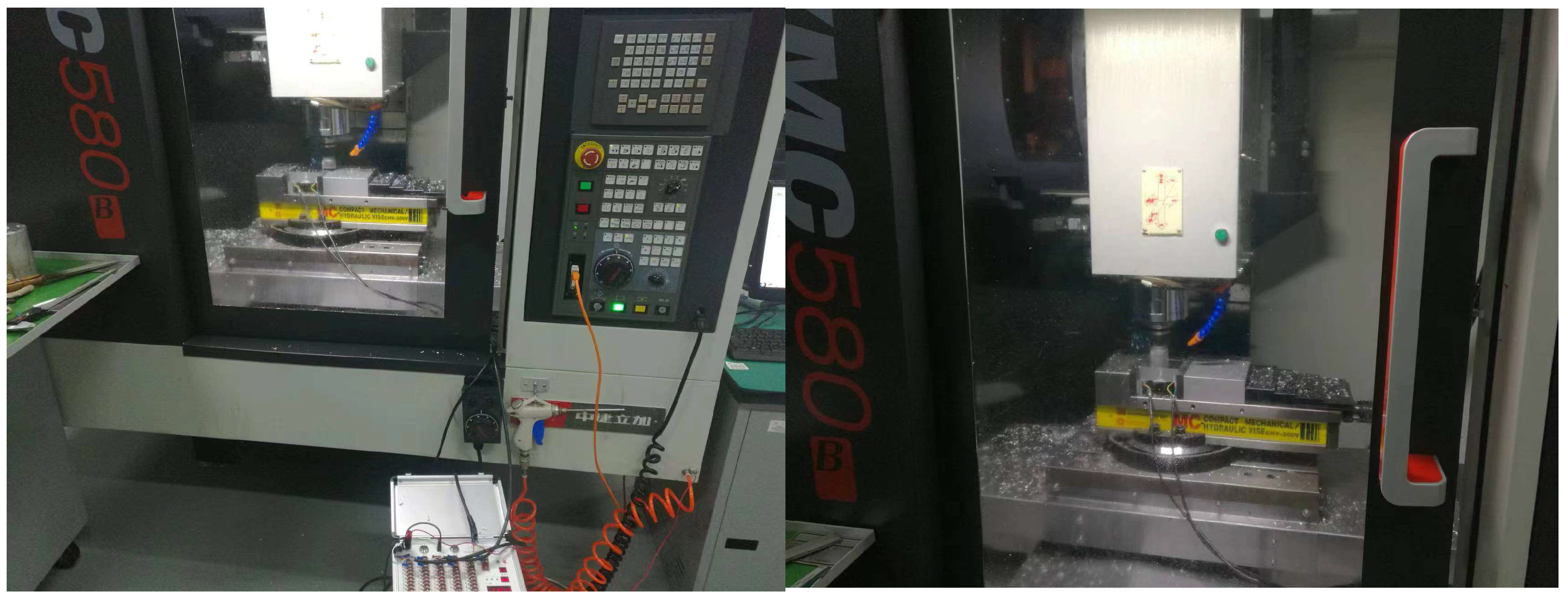
5.5. Experimental Verification

The cutting experiment was conducted on the Shenyang VMC580B vertical machining centre produced by GENERTEC SHENYANG MACHINE TOOL(Shenyang, China). After milling the specimen into the T-shaped component as shown in Figure 11, the deformation of the large flat surface (bottom surface) of the T-shaped component was measured using the MQ8106 Coordinate Measuring Machine (CMM) produced by Xi’an Edwards (Xi’an, China), with a measurement accuracy of 0.0025 mm over 250 mm, as depicted in Figure 15. The experimentally measured flatness error of the bottom surface of the T-shaped component was 0.920 mm. This value differs from the theoretical calculation by only 0.011 mm, an error margin of merely 1.2%, indicating a very close match. This outcome confirms the accuracy of the semi-analytical solution model established for T-shaped components.

6. Conclusions and Prospect

This paper begins with the structural characteristics of T-shaped components, investigates the problem of solving for bending deformation of T-shaped section components under the influence of residual stresses, and arrives at the following conclusions.

(1)

For T-shaped components with relatively thin webs, the calculation of bending deformation under residual stresses can be decomposed into the solutions for bending deformation of T-beams and cantilever plates. The sum of these deformations represents the total bending deformation of the T-shaped component.

(2)

The small deflection bending problem of rectangular cantilever thin plates belongs to linear elastic problems. Its maximum deflection value is related to its geometric dimension and moments subjected. For a rectangular cantilever plate with certain geometric dimension, its deflection value can be solved according to $w=\frac{M_x}{2D}{x}^2$ when the uniformly distributed moments meet $M_y$ = ${\mu M}_x$. While $M_y\ne {\mu M}_x$, the deflection $w$ exhibits a linear variation pattern to $M_y$. And the slopes are different when $M_y>{\mu M}_x$ and $M_y<{\mu M}_x$. The deflection $w$ of rectangular cantilever thin plate shows a non-linear variation patterns to the variation of its dimension ratio ($W/L$).

(3)

An analysis of the impact of residual stresses within the cantilever plate on its dimensional changes and bending deformation has been conducted. This analysis has led to the establishment of a semi-analytical predictive model for the bending deformation of rectangular cantilever plates.

(4)

Experimental validation has confirmed that the semi-analytical solution model developed for T-shaped structural members can accurately calculate the bending deformation of T-shaped thin-walled components under the action of residual stresses. The model demonstrates high solution accuracy and possesses significant engineering application value.

The study focused mainly on the bending deformation of cantilever thin plate and T-shaped aviation aluminium alloy components under residual stress. In the future, the coupling effects between residual stress and other factors, such as temperature changes and load effects, should be considered. Research on coupling effects would prompt the comprehensive understanding of the bending deformation behavior of aviation aluminum alloy components.

References

- Chatterjee, B.; Bhowmik, S. Evolution of Material Selection in Commercial Aviation Industry—A Review. In Sustainable Engineering Products and Manufacturing Technologies; Academic Press: Cambridge, MA, USA, 2019; pp. 199–219. [Google Scholar] [CrossRef]
- Sedeh, M.R.N.; Ghaei, A. The Effects of Machining Residual Stresses on Springback in Deformation Machining Bending Mode. Int. J. Adv. Manuf. Technol. 2021, 114, 1087–1098. [Google Scholar] [CrossRef]
- Zhang, Z.; Luo, M.; Tang, K.; Zhang, D. A New In-Processes Active Control Method for Reducing the Residual Stresses Induced Deformation of Thin-Walled Parts. J. Manuf. Process. 2020, 59, 316–325. [Google Scholar] [CrossRef]
- Aurrekoetxea, M.; Llanos, I.; Zelaieta, O.; López de Lacalle, L.N. Towards Advanced Prediction and Control of Machining Distortion: A Comprehensive Review. Int. J. Adv. Manuf. Technol. 2022, 122, 2823–2848. [Google Scholar] [CrossRef]
- Yi, S.; Wu, Y.; Gong, H.; Peng, C.; He, Y. Experimental Analysis and Prediction Model of Milling-Induced Residual Stress of Aeronautical Aluminum Alloys. Appl. Sci. 2021, 11, 5881. [Google Scholar] [CrossRef]
- Meng, L.H.; Atli, M.; He, N. Measurement of Equivalent Residual Stresses Generated by Milling and Corresponding Deformation Prediction. Precis Eng. 2017, 50, 160–170. [Google Scholar] [CrossRef]
- Sahraei, A.; Pezeshky, P.; Sasibut, S.; Rong, F.; Mohareb, M. Closed Form Solutions for Shear Deformable Thin-Walled Beams Including Global and Through-Thickness Warping Effects. Thin Walled Struct. 2021, 158, 107190. [Google Scholar] [CrossRef]
- Weber, D.; Kirsch, B.; Chighizola, C.R.; Jonsson, J.E.; D’Elia, C.R.; Linke, B.S.; Hill, M.R.; Aurich, J.C. Investigation on the Scale Effects of Initial Bulk and Machining Induced Residual Stresses of Thin Walled Milled Monolithic Aluminum Workpieces on Part Distortions: Experiments and Finite Element Prediction Model. Procedia CIRP 2021, 102, 337–342. [Google Scholar] [CrossRef]
- Li, B.; Dong, Y.; Gao, H. Numerical Simulation and Experiment of Stress Relief and Processing Deformation of 2219 Aluminum Alloy Ring. Metals 2023, 13, 1187. [Google Scholar] [CrossRef]
- Yao, C.; Zhang, J.; Cui, M.; Tan, L.; Shen, X. Machining Deformation Prediction of Large Fan Blades Based on Loading Uneven Residual Stress. Int. J. Adv. Manuf. Technol. 2020, 107, 4345–4356. [Google Scholar] [CrossRef]
- Wang, Z.; Sun, J.; Liu, L.; Wang, R.; Chen, W. An Analytical Model to Predict the Machining Deformation of Frame Parts Caused by Residual Stress. J. Mater. Process. Tech. 2019, 274, 116282. [Google Scholar] [CrossRef]
- Jiang, X.; Wang, Y.; Ding, Z.; Li, H. An Approach to Predict the Distortion of Thin-Walled Parts Affected by Residual Stress During the Milling Process. Int. J. Adv. Manuf. Technol. 2017, 93, 4203–4216. [Google Scholar] [CrossRef]
- Li, Y.; Cheng, X.; Ling, S.; Zheng, G.G. Research on Deformation and On-line Compensation of Straight Micro Thin Walls in Micro Milling Process. J. Hunan Univ. (Nat. Sci.) 2023, 50, 87–96. [Google Scholar] [CrossRef]
- Zheng, Y.; Hu, P.; Wang, M.; Huang, X. Prediction Model for the Evolution of Residual Stresses and Machining Deformation of Uneven Milling Plate Blanks. Materials 2023, 16, 6113. [Google Scholar] [CrossRef]
- Zhu, Y.M.; Mao, K.M.; Yu, X.X. A General Model for Prediction of Deformation from Initial Residual Stress. Int. J. Adv. Manuf. Technol. 2020, 109, 1093–1101. [Google Scholar] [CrossRef]
- Ye, H.; Qin, G.; Wang, H.; Zuo, D.; Han, X. A Machining Position Optimization Approach to Workpiece Deformation Control for Aeronautical Monolithic Components. Int. J. Adv. Manuf. Technol. 2020, 109, 299–313. [Google Scholar]
- Li, Y.; Li, Y.-N.; Li, X.-W.; Zhu, K.; Zhang, Y.-A.; Li, Z.-H.; Yan, H.-W.; Wen, K. Influence of Material Removal Strategy on Machining Deformation of Aluminum Plates with Asymmetric Residual Stresses. Materials 2023, 16, 2033. [Google Scholar] [CrossRef]
- Ju, K.; Duan, C.; Sun, Y.; Shi, J.; Kong, J.; Akbarzadeh, A. Prediction of Machining Deformation Induced by Turning Residual Stress in Thin Circular Parts Using Ritz Method. J. Mater. Process. Tech. 2022, 307, 117664. [Google Scholar] [CrossRef]
- Gao, H.; Li, X.; Wu, Q.; Lin, M.; Zhang, Y. Effects of Residual Stress and Equivalent Bending Stiffness on the Dimensional Stability of Thin-Walled Parts. Int. J. Adv. Manuf. Technol. 2022, 119, 4907–4924. [Google Scholar] [CrossRef]
- Li, X.; Yang, Y.; Li, L.; Zhao, G.; He, N. Uncertainty Quantification in Machining Deformation Based on Bayesian Network. Reliab. Eng. Syst. Saf. 2020, 203, 107113. [Google Scholar] [CrossRef]
- Xue, N.-P.; Wu, Q.; Yang, R.-S.; Gao, H.-J.; Zhang, Z.; Zhang, Y.-D.; Li, L.; Guo, J. Research on Machining Deformation of Aluminum Alloy Rolled Ring Induced by Residual Stress. Int. J. Adv. Manuf. Technol. 2023, 125, 5669–5680. [Google Scholar] [CrossRef]
- Zheng, J.-Y.; Voyle, R.; Tang, H.P.; Mannion, A. Study of Distortion on Milled Thin-Wall Aluminum Parts Influenced by Initial Residual Stress and Toolpath Strategy. Int. J. Adv. Manuf. Technol. 2023, 127, 237–251. [Google Scholar] [CrossRef]
- Li, B.; Deng, H.; Hui, D.; Hu, Z.; Zhang, W. A Semi-analytical Model for Predicting the Machining Deformation of Thin-walled Parts Considering Machining-induced and Blank Initial Residual Stress. Int. J. Adv. Manuf. Technol. 2020, 110, 139–161. [Google Scholar] [CrossRef]
- Li, W.; Ma, L.; Wan, M.; Peng, J.; Meng, B. Modeling and Simulation of Machining Distortion of Pre-bent Aluminum Alloy Plate. J. Mater. Process. Technol. 2018, 258, 189–199. [Google Scholar] [CrossRef]
- Weber, D.; Kirsch, B.; Jonsson, J.E.; D’Elia, C.R.; Linke, B.S.; Hill, M.R.; Aurich, J.C. Simulation Based Compensation Techniques to Minimize Distortion of Thin-walled Monolithic Aluminum Parts Due to Residual Stresses. CIRP J. Manuf. Sci. Technol. 2022, 38, 427–441. [Google Scholar] [CrossRef]
- Wang, H.M.; Qin, G.H.; Lin, F.; Zuo, D.W.; Han, X.; Chen, X.M. A Crossover Iterative Method of Controlling Machining Deformation for 7075-T7451 Aluminum Alloy Thick Plate. Rare Met. Mater. Eng. 2019, 48, 1239–1248. [Google Scholar]
- Li, R.; Zhong, Y.; Tian, B. On new symplectic superposition method for exact bending solutions of rectangular cantilever thin plates. Mech. Res. Commun. 2011, 38, 111–116. [Google Scholar] [CrossRef]
- Guo, K.; Wu, C.; Sun, J. Research progress on NC machining distortion prediction and control technology of aeronautical monolithic components. Aeronaut. Manuf. Technol. 2022, 65, 112–127. [Google Scholar]
- Wang, S.H.; Zuo, D.W.; Wang, M.; Wang, Z.R. Modified layer removal method for measurement of residual stress distribution in thick pre-stretched aluminum plate. Trans. Nanjing Univ. Aeronaut. Astronaut. 2004, 21, 286–290. [Google Scholar]
Figure 1.
Thin plate model.
Figure 2.
Rectangular thin plate loaded with bending moments on two opposite edges.
Figure 3.
Stress model of t-shaped structural component.
Figure 4.
Model of rectangular cantilever thin plate.
Figure 5.
Finite element model of cantilever plate.
Figure 6.
Deflection of rectangular cantilever thin plates under different values.
Figure 7.
Deformation of cantilever plate under conditions.
Figure 8.
Deformation Deflection Values of Cantilever Plates with Varying Width Dimensions.
Figure 9.
Relationship between plate dimension ratio () and deflection.
Figure 10.
Simulation results for model verification.
Figure 11.
T-shaped component.
Figure 12.
Initial Residual Stress Detection Diagram.
Figure 13.
Initial Residual Stress of the Specimen.
Figure 14.
Bending Deformation of T-shaped Component.
Figure 15.
Measurement of Machining Deformation of T-shaped Component.