
Canonical Models of Geophysical and Astrophysical Flows: Turbulent Convection Experiments in Liquid Metals

Abstract
: Planets and stars are often capable of generating their own magnetic fields. This occurs through dynamo processes occurring via turbulent convective stirring of their respective molten metal-rich cores and plasma-based convection zones. Present-day numerical models of planetary and stellar dynamo action are not carried out using fluids properties that mimic the essential properties of liquid metals and plasmas (e.g., using fluids with thermal Prandtl numbers Pr < 1 and magnetic Prandtl numbers Pm ≪ 1). Metal dynamo simulations should become possible, though, within the next decade. In order then to understand the turbulent convection phenomena occurring in geophysical or astrophysical fluids and next-generation numerical models thereof, we present here canonical, end-member examples of thermally-driven convection in liquid gallium, first with no magnetic field or rotation present, then with the inclusion of a background magnetic field and then in a rotating system (without an imposed magnetic field). In doing so, we demonstrate the essential behaviors of convecting liquid metals that are necessary for building, as well as benchmarking, accurate, robust models of magnetohydrodynamic processes in Pm ≪ Pr < 1 geophysical and astrophysical systems. Our study results also show strong agreement between laboratory and numerical experiments, demonstrating that high resolution numerical simulations can be made capable of modeling the liquid metal convective turbulence needed in accurate next-generation dynamo models.1. Introduction
System-scale magnetic fields are observed to develop in galaxies, stars, planets, moons and even asteroids [1–4]. In all these systems, magnetohydrodynamic dynamo action occurs via the conversion of the kinetic energy of flowing electrically-conductive fluids into magnetic field energy [3,5]. Generated by the motion of the electrically-conductive fluid, dynamo fields typically evolve on length and time scales related to the underlying flows [6].
For example, Earth’s geomagnetic field is shown in Figure 1a [7]. The field is predominantly dipolar, with magnetic flux emerging from Earth’s southern hemisphere and returning via the northern hemisphere. The large-scale field cannot be generated in the silicate mantle because temperatures there exceed the Curie temperature of its magnetic minerals at relatively shallow depths, too shallow to generate the 0.1 mT fields observed on the planet’s surface. Furthermore, the fields vary significantly in time (Figure 1b). Such time variations cannot be explained by permanent magnetization of planetary materials. Thus, this strong, spatiotemporally complex magnetic field is best explained via continual magnetohydrodynamic (MHD) induction occurring through the action of turbulent liquid metal flows that exist in Earth’s iron-rich molten outer core (Figure 1c). Similarly, large-scale flows in the sun drive its famous quasi-periodic 22-year magnetic field reversal cycle [9].
However, it is unlikely that there is a simple, direct mapping between flows and magnetic fields in natural dynamo systems. This is predominantly due to the particular material properties of the metallized fluids in which these dynamos are generated.
In galaxies and stars, the electrically-conducting fluid is typically a plasma; in planets and asteroids, the electrically-conducting fluid likely resides within a liquid metal core (Figure 1a). The (inverse) thermal conductivity of the fluid is often characterized non-dimensionally via the Prandtl number,
Indeed, energy is expected to be injected at small-scales via buoyancy-driven convection processes in natural dynamo systems ([11–13]; Figure 1c), and is likely to then cascade upscale to larger scales [14], where we hypothesize that dynamo action likely occurs more efficiently [15] and where large-scale magnetic structures are likely formed. Thus, a detailed understanding of turbulent convection processes in metals is essential for the development of broadly accurate models of geophysical and astrophysical dynamo processes. Unfortunately, relatively little information exists to describe convective turbulence in liquid metals. Even less information exists concerning turbulent convection in liquid metals in the presence of magnetic fields and rotation, as occurs in geophysical and astrophysical settings.
To address this knowledge gap, we have developed a mixed laboratory-numerical platform to investigate the essential properties of small-scale rotating magnetoturbulence in convecting liquid metals. In studies of all types of convecting fluids, an idealized, simplified version called Rayleigh-Beńard convection (RBC) is the canonical, reference system [16]. In RBC, fluid is contained between two co-planar, impermeable boundaries, whose unit normal vectors are aligned with gravity. Typically, the boundaries provide some spatially-uniform thermal forcing, such that an adverse vertical temperature gradient is imposed across the fluid, with warmer fluid underlying cooler fluid. Because the local fluid density is inversely proportional to the temperature, the system releases potential energy when the warm (lower density) fluid becomes convectively unstable to upward motions and the cool (denser) fluid to descending motions.
In order to overcome the magnetic diffusivity of liquid metals and plasmas, generating a dynamo requires either a vast amount of fluid or an extremely strong forcing, e.g., [17]. Instead of studying the generation of a dynamo magnetic field from a turbulent flow, we propose to take the inverse approach and instead investigate the effects of imposed magnetic fields and system rotation on a given RBC system. Thus, we consider such RBC systems to represent idealized parcels of a planet’s or star’s dynamo generation region in which dynamo action does not locally occur, and instead, the magnetic field, assumed to be generated on larger scales, is imposed.
The manuscript is organized as follows. In Section 2, we describe our laboratory experimental device and associated numerical modeling framework. In Section 3, we present the results of a mixed laboratory-numerical investigation of Raleigh-Bénard convection (RBC; non-magnetic, non-rotating) in a cylindrical cavity, using the liquid metal gallium (Pr ≃ 0.025; Pm ≃ 10−6) as the working fluid. (See Table 1 for the thermophysical properties of Ga.) In the parameter ranges accessible to our experiments, turbulent convection in liquid gallium is dominated by large-scale inertially-dominated flywheel-style flows. In Section 4, we show how the imposition of a vertical magnetic field constrains the flow, lessening the inertial effects dominant in the RBC system. In Section 5, we remove the magnetic field and instead rotate the system. Rotation also constrains the fluid dynamics, but mechanically instead of electromagnetically. Rotation leads to oscillatory weakly-nonlinear convective motions and differing heat transfer behaviors than in the magnetoconvection experiments. Finally, in Section 6, we summarize our laboratory-numerical findings and discuss their relevance to our understanding of natural dynamo systems and present-day numerical dynamo models.
2. Laboratory and Numerical Methods
We have developed a new coupled laboratory-numerical tool, well-suited to investigate convective turbulence in liquid metals. Here, we will describe each component of this novel system: first the laboratory experimental device and then the numerical modeling framework.
2.1. Laboratory Experimental Framework
In the laboratory, we have conducted thermal convection experiments using liquid gallium as the working fluid. Our convection tank is a right cylindrical chamber with an outer diameter of 20 cm (see Figure 2a,b). The device can accommodate sidewalls of varying heights. In this study, we have utilized two tank heights, one with a H = 5 cm high stainless steel sidewall (3.0 mm wall thickness) and the other with an H = 10 cm high acrylic sidewall (6.35 mm wall thickness). The 5 cm tank has an aspect ratio Γ ≃ 19.6/5.0 = 3.92 and the 10 cm tank has an aspect ratio Γ ≃ 18.73/10.0 = 1.87, where Γ = D/H is the ratio of the diameter of the fluid layer D versus height H. To minimize heat losses, we thermally insulate the system with a ≃20 cm layer of thermal blanketing that surrounds a 10 cm thick inner layer of closed-cell foam insulation. In addition, several thermocouples are inserted within these layers in order to quantify heat losses.
As shown in Figure 2a, the bottom thermal block consists of a 1 cm thick copper plate; and the top thermal block consists of a 2.5 cm thick copper plate. In order to determine the full temperature difference across the fluid layer, ΔΘ, the top and bottom thermal blocks each contain 6 lid thermistors, homogeneously distributed in azimuth, and located 1 mm above and below the fluid layer, respectively. In addition the top thermal block has 5 thru-holes (Figure 2b) allowing us to insert thermistors of various lengths into the fluid interior. In the 5 cm high tank, the internal thermistors are located at depths of: 4 cm (T1), 1cm (T2), 2.5 cm (T3), 1 cm (T4) and 1.25 cm (T5). In the 10 cm high tank (not shown in Figure 1), the internal thermistor depths are: 5 cm (T1), 2.5 cm (T2), 5 cm (T3), 1.5 cm (T4) and 2.5 cm (T5). The internal thermistors have depth tolerances of ±0.5 mm. T3 is always located at the center point of the tank. The other thermistors allow us to measure the 3D structure of the temperature field.
The fluid must be heated from below and cooled from above to drive thermal convection in the fluid layer. Thus, the device has a 19 cm diameter, non-inductively wound, electrical resistance heater, capable of delivering 4900 W of heating power, that is attached to the base of the bottom thermal block (Figure 2a). The heat is removed by a water-based heat exchanger that is situated above the top thermal block. The attached cooling block is a right cylinder of aluminum into which has been cut a double wound spiral flow channel. This double wound spiral acts to minimize temperature gradients in the block [18]. The temperature of the water is thermostated by a precision chiller capable of removing up to 10 kW of heating power while maintaining the bath temperature between a 5°C and 35°C, stable to within ±25 mK.
Temperature data is acquired via a digital data acquisition system capable of simultaneously sampling up to 32 thermistor channels, typically at a sampling rate of 10 Hz. In addition, 32 more channels are available to measure temperatures via K-type thermocouples, which we use to evaluate thermal losses and to monitor ambient temperature in the room.
In laboratory convection systems, it is important to ascertain the thermal properties of the boundaries, in order to be comparable with theoretical models, cf. [21]. To evaluate the thermal boundary conditions, we determine the value of the Biot number, Bi, for the top and bottom thermal blocks. The Biot number, which is the ratio of the effective thermal conductance of the fluid layer and the boundary material, is defined as:
For Biot number values less than ≃ 0.1, the thermal boundaries typically remain isothermal to within a few percent [22]. Our experimental Bi values fall within this range (Bi ≲ 0.1), such that both thermal boundaries should be treated as being isothermal. These arguments are verified by our laboratory magnetoconvection and rotating convection experiments, in which convection first onsets in accordance with linear predictions for isothermal boundaries. This was also found to be the case in a preceding study of rotating convection in a larger volume tank of gallium [20].
The entire device described above is situated on a rotary table that is belt-driven by a 10 N.m brushless servomotor. The device can be rotated between 0.1 and 2π rad/s (i.e., 0.5 to 60 revolutions per minute), steady to within ±0.1%.
A 35 cm bore solenoidal electromagnet is situated in the (non-rotating) lab frame and can be lowered on jack screws around the convection tank. The solenoid can supply a vertical, imposed magnetic field of up to 0.1325 T that is uniform to within ±0.5% over the volume of our largest gallium convection tank, which is approximately 20 cm3.
Thus, this laboratory experimental device allows us to investigate turbulent convection in liquid metal subject to magnetic forces, rotational forces as well as their combined effects, as are all relevant to our understanding of natural systems. For further device details, we refer the reader to [23].
2.2. Numerical Modeling Framework
In close association with our laboratory experiments, we have carried out numerical simulations using a modified version of the SFEMaNS code, which has been used previously in studies of mechanically-forced magnetohydrodynamic flows in liquid metals [24–26]. SFEMaNS is a hybrid code that makes use of Fourier series in the azimuthal direction. In meridian planes, it uses nodal quadratic Lagrange finite elements for the velocity field and nodal linear Lagrange finite elements for the pressure field. The discretization of time is made by means of a semi-implicit, second-order backward finite difference method (BDF2). This code is efficiently parallelized in Fourier space and on meridian sections (see Appendix 1). The domain decomposition is made using METIS [27], and the parallelization is made using MPI and PETSC libraries [28,29]. The code’s unstructured meridional mesh, shown in Figure 2c, allows SFEMaNS to be used to simulate MHD flows in any axisymmetric geometry.
The key modification we have made to the code is the inclusion of a thermal field solver, allowing for thermally-driven MHD simulations of Boussinesq fluids in which the density is constant except in the buoyancy term [30,31]. This new version of the code, called SFEMaNS-T, has already been used successfully to simulate convection-driven, planetary dynamo action in a spherical shell geometry in the community benchmarking exercise of [32].
In this study, we carry out numerical calculations in right cylindrical geometries (see Figure 2c,d). The numerical tank geometries are nearly identical to our laboratory experimental cases, with numerical aspect ratio values of Γ = 2 and 4. The points P1 through P5 (shown in Figure 2c,d) represents numerical probes that are directly equivalent to the laboratory thermistors T1 through T5 (shown in Figure 2a,b), allowing point-to-point comparisons of the temperatures in each system.
Within the fluid layer, denoted as domain I in Figure 2c,d, SFEMaNS-T simultaneously evolves the velocity, thermal and magnetic fields by solving the Boussinesq forms of the Navier-Stokes momentum conservation equation in a reference frame rotating at constant angular velocity ; the energy conservation equation; and the magnetic induction equation, derived from Maxwell’s equations under the MHD approximation in which the velocities of the electrically-conducting fluid are assumed to be far less than the speed of light. For detailed derivations of these equations see [33–35].
The non-dimensional governing equations that SFEMaNS-T iteratively solves are
In the momentum Equation (4), the left hand side terms give the Lagrangian acceleration of the fluid. The terms on the right hand side are, respectively, the pressure gradient force (per unit volume), the buoyancy force, the viscous force, the Lorentz force and the Coriolis force. The centrifugal force is absorbed inside the pressure term. Lorentz forces arise in this via a uniform, axial magnetic field that can be imposed. Similarly, the system can axially rotate at a steady angular velocity , leading to Coriolis forces.
In the energy Equation (5), the Lagrangian time derivative is on the left hand side and thermal diffusion is on the right hand side. As there are no internal buoyancy sources in this system, the thermal buoyancy forcing must be maintained by the thermal boundary conditions.
In the magnetic induction equation (6), the magnetic field is generated by the first term on the right hand side, the “stretching” term, and it is diffused by the second term on the right hand side. Flows can generate magnetic fields, but in doing so, they generate Lorentz forces that act back on the velocity field such that system’s total energy is conserved.
Non-dimensional control parameters are grouped in front of the various terms of Equations (4)–(6). To arrive at these groups, we have non-dimensionalized the governing equations in the following way. Velocities are scaled using the free-fall velocity estimate for an undamped thermally buoyant parcel that traverses the fluid layer,
We have previously defined the two Prandtl numbers that non-dimensionally describe the fluid properties. Three other non-dimensional control parameters arise in Equations (4)–(6). The Rayleigh number
When Ra is large, buoyancy effects dominate over diffusion. The Chandrasekhar number,
For the velocity field, non-penetrative, non-slip conditions are applied on all the boundaries of fluid layer, which is denoted as domain I in Figure 2c. The non-dimensional temperature Θ is scaled by the vertical temperature difference ΔT. The top and bottom boundary conditions are isothermal with values of
In order to correctly solve for the magnetic field, the fluid region is surrounded by a “vacuum” region, denoted as domain II in Figure 2c,d. In the vacuum, no electrical currents can exist and, thus, the magnetic field satisfies a potential field solution. The continuity of the magnetic field between domains I and II is weakly imposed on the interfaces Σ2, Σ4 and Σ5 in Figure 2c,d through an interior penalty method, e.g., [24]. The magnetic field is set to zero on the outer boundary of domain II. Our finite element solution requires no special conditions to be imposed along the axis of rotation.
We set the initial temperature field to the diffusive solution:
2.3. Convective Free-Fall Parameters
The control parameters in Equations (4)–(6) are the same as those used to describe the laboratory experiments. However, Pr, Q and E are all ratios relative to diffusive time-scales, whereas we have non-dimensionalized the equations using the (strongly turbulent) free-fall velocity and time scales, Uf and τf. To better account for this choice of free-fall non-dimensionalization, we define the following “convective” parameters.
The convective Reynolds number is defined as
When Rec is large (and constraining magnetic and rotation forces are comparatively small), then fluid inertia dominates viscous diffusion of momentum and the convective flows are turbulent [36]. The convective Peclet number is defined as
Large values of Pec imply that thermal advection processes dominate thermal diffusion effects. In such cases, thermal turbulence tends to mix and often isothermalize the interior of the convective fluid layer, e.g., [16]. The convective magnetic Reynolds number is defined as
For small Rmc, Ohmic dissipation dominates magnetic induction such that the magnetic field never greatly differs from the imposed field for large Rmc, induction can dominate and self-sustaining dynamo action can become possible [5,33]. The convective interaction parameter is
This parameter estimates the ratio of Lorentz and inertial forces in the momentum equation. For large Nc, Lorentz forces dominate fluid inertia [33,34]. The convective Rossby number predicts the ratio of fluid inertia and Coriolis force and is defined as
For small RoC, convective turbulence is likely to be constrained by the effects of rotation, e.g., [37].
With these free-fall-based parameters, the governing equations are then re-cast as:
In the following sections, we will present our results typically in terms of the standard parameters Ra, Q and E. We will typically use the standard parameters when describing physical phenomena occurring near to the onset of convection, where molecular diffusive effects are often relevant. In contrast, we will usually interpret the physics using the convective Reynolds number based parameters (16)–(20) in fully-developed, turbulent cases in which the flow speeds may be approaching Uf and advection processes overwhelm diffusive transport phenomena, cf. Table 2.
3. Compilation of Heat Transfer Measurements
The behavior of thermal convection systems is often characterized by measurements of the efficiency of global heat transfer across the fluid layer. This heat transfer efficiency is parameterized by the non-dimensional Nusselt number, Nu, which is the ratio of total heat transfer to that transported only by thermal conduction,
For weak buoyancy forcing (i.e., sufficiently low Ra), the fluid layer is stable and perturbations in the flow and temperature field will decay to zero. Thus, the vertical velocities will tend to zero and the heat flux must diffuse across the fluid layer via thermal conduction alone, such that Nu = 1. Then at the so-called critical Rayleigh number, Racrit, the fluid in the layer becomes gravitationally unstable and convective motions onset. Warmer fluid parcels will tend, on average, to rise through the fluid layer and colder fluid parcels will tend to fall, releasing gravitational potential energy stored in the initial configuration of the density field in which least dense fluid lies at the base of the fluid layer. These convective motions advect heat across the fluid layer and the Nusselt number will tend to increase above unity. In order to measure Nu in our laboratory experiments, we obtain measurements of the total temperature difference, ΔT, across the thermistors embedded in the top and bottom thermal blocks, and the heat flux, q supplied by the basal heat pad. The material properties of the liquid gallium, such as k, are calculated as in [20].
Figure 3 is a compilation of all our heat transfer measurements. The non-dimensional buoyancy forcing, Ra, is plotted on the x-axis versus the heat transfer efficiency, Nu, on the y-axis. Rayleigh-Bénard convection experiments are demarcated by open square symbols. Magnetoconvection (MC) experiments, carried out at fixed Chandrasekhar number Q = 3.5 × 10³, are marked by diamond shaped symbols. Lastly, rotating convection (RC) experiments, all made using a fixed Ekman number of E = 2 × 10⁻⁵, are represented by circular symbols. Open symbols denote laboratory experimental results and red-filled symbols correspond to numerical simulation results. The colors of the symbol lines express the fluid layer geometry: black lines correspond to Γ ≃ 4 cases; blue corresponds to Γ ≃ 2 cases; and green corresponds to Γ ≃ 1 cases. (The Γ ≃ 1 rotating convection laboratory data is from the study of [20].)
The three different suites of experiments, RBC, MC and RC, all show significant differences in their heat transfer behaviors. The lowest value of Nu in the RBC data set is near two. Exceeding Nu = 1, this implies that the Rayleigh numbers investigated in this set of experiments all exceed the critical Rayleigh number for RBC. In addition, the RBC data appears to display a single power law behavior, suggesting that we are interrogating a single behavioral regime of liquid metal convection. This scaling behavior is discussed in detail in Section 4.
In contrast, the Nu-Ra data shows that the zeroth order effect of either an imposed magnetic field or an imposed system rotation is to stabilize the layer of liquid metal against convective motions. In the MC cases, the critical Rayleigh number is just below Ra = 3 × 10⁴. In the RC cases, convection onsets closer to Ra = 1.5×10⁵. After convection onsets in the MC and RC systems, the heat transfer behaviors are more complex than in the RBC experiments. Just after the onset of convection, the MC Nu data rises sharply with Ra and has a concave downward curvature until, at a sufficiently high Rayleigh number of about 106, the MC data merges with the RBC data. In contrast, the RC data has a very shallow slope just after convection onsets. This gives way to a steeper trend at close to Ra = 106, which then intersects with the RBC data in the vicinity of Ra = 107.
The data in Figure 3 shows that the MC and RC return to the RBC trend at sufficiently high Ra. Qualitatively, this behavior is unsurprising: MC systems behave similarly to RBC systems when Nc is sufficiently low and RC systems behave similarly to RBC systems when Roc is sufficiently high. Thus, the RBC heat transfer data provides an approximate upper bounding curve the MC and RC heat transfer data sets. This further implies that knowledge of RBC convective scaling behavior is necessary to understand the behaviors of the MC and RC systems. A similar result exists for rotating convective heat transfer in moderate Pr fluids, such as water [13]. Thus, the import of understanding RBC as the essential basis for more complicated convection systems holds broadly.
In the following three sections, we will consider in greater detail the behaviors of Rayleigh-Bénard convection in liquid metal, magnetoconvection and then rotating convection.
4. Rayleigh-Bénard Convection (RBC)
4.1. Essential Theory
Without the effects of magnetic fields or background rotation, the governing equations for RBC simplify to
In strongly forced (high Ra) convection systems, buoyancy-driven flows develop with relatively high convective Reynolds numbers, For Rec values above roughly 103, multi-scale, three-dimensional (3D), turbulent motions will tend to develop in RBC systems. However, in liquid metals, the low value of Pr means that the may remain low even in relatively high Rec settings, e.g., [39]. Because of this, strong convective flows in liquid metals (e.g., Re ≳ 103; Pe ≲ 103) will often be unable to strongly mix the thermal field. Instead, such flows will tend then to create large amplitude, large scale temperature perturbations in the fluid bulk (e.g., see Figure 1c in [40]). Vigorous small-scale flows in liquid metals will be largely unable to perturb the thermal field.
In RBC, convective heat transfer is parameterized via scaling laws predicting the value of the Nusselt number, Nu, as function of Ra and Pr:
In moderate Prandtl number convection (Pr ≳ 1), studies often find the heat transfer is controlled by boundary layer physics resulting in α values between 2/7 and 1/3 [13,16,36,41,42]. The α ≃ 1/3 law is predicted to arise under the following when vigorous convective mixing creates a nearly isothermal fluid bulk (Pec ≫ 1). Then the temperature gradients in the fluid become concentrated into the quasi-static regions of thickness δ that exist adjacent to the top and bottom boundaries (where impenetrability requires uz → 0). In these boundary layers, the heat transfer is dominantly diffusive and the temperature drop, δT, across each of these regions must scale as δT ≃ 1/2ΔT. Then the Nusselt number can be re-cast as
If it is assumed that the thermal boundary layers operate independently of one another at large Nu, then the heat transfer should be independent of the fluid layer depth H, e.g., [43]. For fixed Pr, dimensional analysis then requires Nu ∼ Ra1/3 [43–45]. This result is indeed found in experiments carried out at Ra ≳ 1010; Nu ≳ 100.
At lower Ra values, it is typically found that RBC heat transfer follows a Nu ∼ Ra2/7 scaling. It was first postulated by Shraiman & Siggia (1991) [46] that this α ≃ 2/7 scaling occurs when the boundary layers are subjected to a large-scale shear flow. They argue that this shear is typically produced by large-scale circulations, making the heat transfer dependent on the container geometry. In this α ≃ 2/7 regime, the heat transfer is still controlled by the boundary layer physics, but the shear modifies the heat transfer efficiency (Recent, two-dimensional convection simulations by Goluskin et al. (2014) [47] suggest that such shear inhibition effects may be capable of lowering the heat transfer coefficient well below 2/7.)
In sharp contrast, boundary layer processes do not necessarily control the heat flux in low Pr fluids. Instead, heat transfer is controlled by large scale flows in the fluid bulk. Strong bulk flows naturally arise in low Pr fluids because inertial effects can dominate the system even at the onset of convection [48]. Various laboratory and numerical studies have shown that convection in liquid metals or low Pr fluids tends then to be dominated by inertial flywheels [49]. In an inertial flywheel, the fluid motions cascade upward in scale, nearly to the size of the container, and approach the free-fall velocity of the system in which fluid buoyancy is transferred directly into inertia. However, such high Rec, moderate Pec flows are unable to isothermalize the fluid bulk, as in moderate Pr fluids. Instead, these high velocity, large scale flows are able to generate container-scale gradients in the perturbation temperature field [40,50].
It is hypothesized that in these low Pr, inertial flows heat transfer will follow an α = β = 1/4 heat transfer law [20,49]. This scaling behavior arises from a balance between thermal advection by the inertial flywheel flows and thermal diffusion across the quasi-static boundary layers:
Substituting in the free-fall velocity relation (7) and using equation (28) leads to
Note that low Pr inertial flywheel flows are predicted to transfer heat less efficiently (α ≃ 1/4) than convection occurring in moderate Pr fluids (α ≃ 1/3). Heuristically, this difference in α values arises because the rate at which heat is transferred across the fluid layer in inertial systems depends on both the free fall time τf necessary to advect heat across the fluid layer and the time needed to diffuse heat across the thermal boundary layers. In contrast, in moderate Pr convection, the rate of heat transfer is higher because it depends only upon the time needed to diffuse heat across the thermal boundary layers as heat is shunted directly across the isothermal interior fluid.
However, the inertial heat transfer scaling (30) is not firmly established in the liquid metals literature. In fact, experiments in liquid metals have yielded a wide range of results providing α values from 1/5 up to 1/3 [18,20,51–54]. This broad range of possible α values shows that heat transfer in liquid metals is not as well understood as it is in moderate Pr fluids [16].
In our RBC experiments presented below, we show that a α ≃ 1/4 scaling law best fits the heat transfer data over the range 2 × 10⁴ ≲ Ra ≲ 3 × 10⁷. Further, we demonstrate that large-amplitude temperature variations arise on the scale of the various inertial flywheel morphologies that develop in our experiments. Irrespective of the morphology of the flywheel flows, we find a the mid-plane thermal anomaly to remain near to 60% of the vertical temperature difference across the fluid layer.
4.2. Experimental Results
Along with twenty-seven laboratory experiments (Table 3), we have carried out four fully three-dimensional numerical simulations, through made using SFEMaNS-T (Table 4). The input parameters in these numerical cases correspond closely to the four laboratory experimental cases demarcated through in the left hand column of Table 3.
In Figure 4, we plot the Nu-Ra data from all laboratory and numerical experiments. Hollow symbols represent laboratory data; red-filled symbols represent numerical simulation results. Square symbols connote a 5 cm high fluid layer, corresponding to a Γ ≃ 4 tank geometry; diamond-shaped symbols connote a 10 cm high fluid layer, corresponding to a Γ ≃ 2 tank geometry; circular symbols connote a 20 cm high fluid layer, correspond to a Γ ≃ 1 tank geometry.
The combined laboratory-numerical data set, over the range 2 × 10⁴ ≲ Ra ≲ 3 × 10⁷, is best fit by the power-law:
The data match the predicted heat transfer law (30) describing inertial convection in low Pr fluid, Nu = 1/2(RaPr)(1/4). In fact, this fit agrees with the theoretical prediction to within ≃14% of the value of the coefficient and to within ±0.4% of the predicted value of the exponent.
This quantitative agreement with theory demonstrates that inertial convection transfers heat via the predicted 1/4 scaling law in the range of parameters investigated here. This finding appears theoretically sensible based on the values of Rec and Pec accessed in our experimental range. For instance, inertial flywheel flows should be expected to develop as 860 ≲ Rec ≲ 3.6 × 10⁴ in our RBC experiments. In contrast, the convective Peclet number range is far more moderate, covering 20 ≲ P ec ≲ 830. In Γ = 1/2 RBC experiments in liquid mercury, Glazier et al. (1999) [41] found that the 1/4 scaling law broke down to a 2/7 scaling at higher Ra values, typically exceeding ∼ 109.
We also find good quantitative agreement between the local temperature measurements in the laboratory and numerical experiments. For example, Figure 5a shows the non-dimensional temperature time series, Θ, acquired on thermistors T3 (black line) and T5 (grey line) in the laboratory experiment, here with temperatures normalized by ΔT. The corresponding Θ time series are also plotted on the point probes P3 (red line) and P5 (green line) from the corresponding numerical simulation . There is good agreement between mean values at locations 3 and 5. The low frequency behaviors of the time series are also comparable between the two system. High frequency temporal variations in the laboratory data are not present in the numerical simulations with variances in the temperature measurements differing by up to 50%.
The strong agreement we find between all the laboratory-numerical internal mean temperature measurements implies that the same large-scale flow structures develop in our numerical simulations and in each associated laboratory experiment. Thus, the numerical simulations provide a means to indirectly visualize the large-scale flows that develop in the optically opaque liquid gallium laboratory experiments.
The agreements of laboratory-numerical point-by-point temperature measurements, as well as global heat transfer measurements, serve as a benchmark and provide cross-validation of the two approaches. Figure 5b further underscores the laboratory-numerical cross-validation. In this panel, we plot the time-averaged, non-dimensional temperature on each thermistor (i.e., 〈Θ(Ti) 〉t for the ith thermistor), normalized by the time-averaged, non-dimensional temperature of the corresponding numerical point-probe (〈Θ(Pi)〉t). The values of this ratio are close to unity (within ±5%) on all five thermistor/point-probe pairs, in each of the four RBC comparison cases. For such pointwise agreement to occur, the large-scale thermal and flow structures must be similar across all our laboratory-numerical comparison cases, further validating our coupled approach.
We find that inertial flows develop in all four numerical simulations. The convective flows reach speeds near the free-fall estimate. This is shown in Figure 6a, which plots the typical maximum velocity amplitude, |Uz|,
Because Pr ≪ 1, these strongly inertial flows exist at only moderate Pec, and thus might be expected to be inefficient at advecting temperature anomalies across the fluid bulk. Instead, large-scale, large-amplitude thermal anomalies are generated in the bulk (cf. [40,50]). Figure 6b shows the time-averaged, maximum horizontal thermal anomaly on the mid-plane, |δζ|,
Figure 7 shows the results from snapshots of numerical simulations carried out in Γ = 4 fluid layer geometries, with case results displayed in the left hand column and case results displayed in the right hand column. The top row of images, Figure 7a,c, show snapshots of the temperature anomaly field on a meridional slice through the fluid layer. Red color contours represent anomalously warm fluid, while blue contours represent anomalously cool fluid. In addition, three-dimensional streamlines in the vicinity of this meridional plane are also rendered. The color of the streamlines demarcates the local vertical flow velocities, with red denoting upward flow, and blue denoting downward flow. Figure 7b,d give oblique views of the temperature anomaly field on the mid-plane of the fluid layer, again, with 3D streamlines rendered through the fluid volume. The black dashed lines in each panel mark the intersection of the meridian plane with the mid-plane, respectively, in Figure 7a,d and in Figure 7c,d.
The streamlines in Figure 7b show that three inertial convection cells span the fluid layer in case . Upward flow velocities correspond to warm fluid being advected towards the top boundary; downward flow velocities advect cold fluid downward. This azimuthal wavenumber m ≃ 3 thermal and flow pattern is in good agreement with the temperature profiles shown in Figure 7a. We find the horizontal temperature differences on the mid-plane of the fluid reach values of ≃60% of the imposed vertical temperature difference, verifying the |δζ| value for the case shown in Figure 6b. The oblique view in Figure 7c shows that the convection pattern is not dominantly axisymmetric in this case. The scatter in the dash ied snapshot profiles in Figure 7a is produced by precession and low-frequency variations of the non-axisymmetric convection pattern displayed in Figure 7c.
In sharp contrast to case , the more strongly forced case develops a predominantly axisymmetric flow pattern with a large-scale upwelling along the centerline (r = 0) of the fluid layer and downward flows along the container sidewalls. As shown in Figure 7d, this large-scale axisymmetric, inertial circulation (with power dominantly at m = 0 and subdominantly at m = 4) generates similarly strong horizontal temperature gradients on the mid-plane of the fluid, again, approaching 60% of the imposed vertical temperature gradient. The decrease in dominant horizontal mode number from m = 3 in case to the axisymmetric mode in case is reminiscent of the inferred change in mode number in the Γ = 4.5 liquid sodium convection study of [53].
Figure 8, constructed in parallel to Figure 7, shows results from numerical simulations carried out in Γ = 2 fluid layers, with case results displayed in the left hand column and results displayed in the right hand column, shown in Figure 8c,d.
Figure 8a,b shows that a complex, non-axisymmetric flow structure, dominantly characterized by a mode number m = 2 pattern, develops in case . Case , which has the highest Ra value and relatively low aspect ratio of Γ = 2, yields a classical large-scale circulation (LSC), with a single non-axisymmetric m = 1 inertial cell dominating the fluid domain [55–57]. The meridional slice in Figure 8c shows upwelling, warm fluid on one side of the container and downwelling, cool fluid on the opposite side. The oblique, snapshot view in Figure 8d shows that the LSC is spatially well-constrained, circulating about a relatively well-defined axis. This m = 1 flow pattern generates an approximately monotonic mid-plane temperature profile, and, yet again, generates maximum mid-plane temperature anomalies of |δζ| ≃ 0.6 (Figure 6b).
The large-scale structures forming in our experiments are produced by a so-called inverse cascade process, in which turbulent convection excites small-scale modes that drive larger-scale inertial modes [49,58]. These inertial modes can approach the size of the fluid domain (Figure 8c). We have carried out lower resolution numerical test cases that do not contain small-scale modes and find that these cases fail to generate large-scale structures. This implies that upscale fluxes are important to the formation of large-scale structures in our convection experiments. Such cascades can also occur in sufficiently turbulent convection in moderate Pr fluids, including water [16] and air [59]. However, these moderate Pr LSC flows generate relatively large Pec values and, thus, tend to thermally mix and isothermalize the bulk fluid. These Pr ≳ 1 LSC flows, then, do not generate such strong mid plane temperature anomalies, as are found here as well as in other comparable low Pr convection studies [40,50].
Our strongly inertial low Pr flows generate rather moderate values of Pec, and thus are expected to be inefficient at generating small-scale temperature anomalies in the fluid. In contrast, though, we find that large-scale flywheels are extremely well-suited at generating significant large-scale temperature anomalies throughout the convecting layer of liquid metal. Heuristically, these large-scale flows advect the large-scale temperature field with little small-scale thermal mixing effects. Low Pec inertial flywheels act, effectively, to rotate the imposed background temperature gradient around the flywheel’s horizontal rotation axis, thereby generating large thermal anomalies in the bulk which exceed those found in lower thermal conductivity (higher Pr) fluids.
The strong thermal anomalies that arise in liquid metal RBC experiments produce remarkably clean temperature time series. Figure 9 shows temperature time series recorded on the central thermistor T3 in the left hand column and associated Fourier spectra in the right hand column. The top row, labeled a, shows the results from the laboratory case; the bottom row, labeled b, corresponds to the case. The time series panels plot temperature in degrees Celsius as a function of time normalized by the thermal diffusion time scale, t/τκ. Both cases were made in the Γ = 1.87 tank with H ≃ 10 cm, for which the thermal diffusion time is τκ ≃ 13 minutes. Strong, quasi-periodic temperature oscillations arise in both cases.
In the Fourier spectra plots, frequency is normalized by the predicted overturn frequency of a container scale (n = 1) LSC, which we estimate in the following way. The typical time for a parcel, traveling at near the free-fall velocity, to make a vertical traverse of the the container is τf = H/Uf. Roughly maintaining that speed, the time for a parcel to circulate around a given large-scale convection cell is
The results of associated numerical case predicts that the dominant frequency in the case should be characterized by that of an (n = 1) LSC. In contrast, the simulation vacillated between the two roll, n = 2 state shown in Figure 8a,b, and a single roll n = 1 LSC state. Thus, these Γ = 2 numerical models predict that the spectrum in the case should have a single dominant peak at f/fLSC ≃ 1, whereas the spectrum in the should contain power at f/fLSC ≃ 1 for the n = 1 LSC flow as well as at f/fLSC ≃ 3/2 for the n = 2 state.
The peaks of the Fourier spectra in Figure 9b,d agree well with predictions based on our visualizations of the corresponding SFEMaNS-T cases and shown in Figure 8. The fact that the SFEMaNS-T results successfully predict the laboratory thermistor Fourier spectral content likely provides the strongest cross-validation of our coupled laboratory-numerical modeling environment. Further, it implies that we can interpret strong peaks in laboratory Fourier spectra in terms of the morphological structure of the flywheels that develop in inertially-dominated convection cases.
In the RBC cases presented here, we have shown broad agreement between theoretical predictions, laboratory measurements and numerical modeling results. However, the fixed strength of |δζ| ≃ 0.6 found here is particularly surprising. One-dimensional scaling theories fail to predict a fixed value for the large-scale temperature anomalies on the mid-plane. For example, modifying the low Pr scaling arguments of [60] to make use of equation (30), we predict that the mid-plane anomalies will decrease approximately as |δζ| ∼ (RaPr)−1/4 ∼ Nu−1. However, this behavior is clearly not verified by our SFEMaNS-T simulation results, nor those of [40,50]. This |δζ| ≃ 0.6 result must, however, break down in the limits of either small Pr → 0, where the temperature field must asymptote back to the diffusive profile, or large Pec, where the bulk fluid becomes isothermalized. Advanced theoretical descriptions of low Pr, moderate Pec heat transfer dynamics should aim to describe this apparently unique feature of Rayleigh-Bénard convection in liquid metals.
5. Magnetoconvection (MC)
5.1. Essential Theory
We have carried out a laboratory-numerical suite of non-rotating, magnetoconvection (MC) experiments, using vertically-imposed magnetic fields with Chandrasekhar number Q ≃ 3.5 × 10³ (see Figure 10 and Tables 5 and 6). In our Γ ≃ 2 and Γ ≃ 4 laboratory experiments, this Q value corresponds to imposed magnetic field strengths of Bo = 13.0 mT and Bo = 26.0 mT, respectively. See Tables 5 and 6 for all the MC case parameter values.
The governing equations for the MC system are
To understand the effects of the magnetic field, we first estimate the convective magnetic Reynolds number, Rmc. At the highest Ra reached in our experiments, Rmc ≲ 10−2. For Rmc ≪ 1, the imposed magnetic field is not significantly induced or advected by the flows in our experiments. The imposed field in a Rmc ≪ 1 fluid remains effectively invariant; induced fields are negligible and the magnetic diffusion time-scale drops out of the problem. In this low Rmc limit, it is not necessary then to solve equation (37). Instead, it is possible estimate the Lorentz forces by calculating the induced currents using Ampere’s law in an electrically conductive fluid,
Applying the quasi-static approximation, the Lorentz force becomes
Under this approximation, the Lorentz force acts only on u⊥, the horizontal velocity component perpendicular to . Further, the Lorentz force acts to oppose these motions, providing a magnetic drag on the horizontal flows that acts with a characteristic drag time-scale .
Since the low Rmc Lorentz force acts like an anisotropic magnetic viscosity, e.g., [19,34,60], in the limit of high Q, the onset of convection is no longer sensitive to the fluid’s molecular viscosity ν. Instead, the critical Rayleigh number for magnetoconvection in an asymptotically strong vertical magnetic field is found to grow in proportion to the strength of the Lorentz force [34,38]:
This predicts that MC will onset at in our Q = 3.5 × 10³ experiments.
The strong damping of horizontal flows acts to decrease the horizontal scale of overturning convection cells at the onset of magnetoconvection. Thus, for Q ≫ 1, the plane layer theory predicts that the onset width of MC cellular flows, non-dimensionalized using the fluid layer depth H, is [38]
Thus, the horizontal length scale of overturning convective motions (i.e., half of a traditional wavelength), is expected to be lQ ≃ 0.43 in our experiments. Using this estimate derived for an infinite horizontal layer, we estimate that roughly n ≃ Γ/lQ ≃ 10 steady cellular structures will span a diameter in our Γ ≃ 4 cylindrical experiments near convective onset. Similarly, we estimate an azimuthal wavenumber m = πΓ/(2lQ) ≃ 15.
Once magnetoconvection begins to occur, the convective heat transfer will be hampered by damping effects of the magnetic fields. In order then to provide a rough prediction of the transition between the Lorentz-dominated MC regime and the undamped, inertial-dominated regime, we non-dimensionalize equation (39) and substitute it into equation (35) in place of Nc(∇×B)×B. This leads to the quasi-static equations for the MC system:
The non-dimensional parameter N is the interaction parameter in the quasi-static, low Rmc limit and is the ratio of the free-fall and Lorentz drag time scales,
The value of N decreases below unity in our experiments in cases with Ra ≳ 3 × 10⁵. These low Rmc arguments predict that the Lorentz forces will restrict the convective motions and the associated convective heat transfer at Ra ≲ 3 × 10⁵, whereas at higher Ra, the MC flows will be effectively undamped and RBC-style inertial heat transfer will occur.
A number of MC investigations have considered low Rmc heat transfer scaling laws in the magnetically-controlled N ≳ 1 regime [19,60–62]. With data at only one value of Q, we will put forward qualitative descriptions of MC heat transfer here. More detailed arguments will require data covering broader ranges of both Ra and Q.
5.2. Experimental Results
A total of 21 MC experiments have been carried out at Q ≃ 3.5 × 10³, 16 laboratory and 5 numerical cases (see Tables 5 and 6). The laboratory and numerical experimental set-up are nearly identical, with the largest difference existing between the value of the laboratory magnetic Prandtl number, Pm ≃ 1.5 × 10⁻⁶, and the numerical magnetic Prandtl number, Pm = 10−4. The Nu-Ra-Q data is plotted in Figure 10, following the same conventions as in Figure 3. In all but the highest Ra MC cases, the heat transfer is suppressed relative to RBC cases at comparable Ra values. In fact, convective heat transfer is completely stifled such that Nu ≃ 1 for Rayleigh number values that are below the predicted critical value For , the heat transfer rises sharply with Ra, but with a negative curvature to the Nu-Ra trend (cf. [60]). The behavior of the MC heat transfer data merges with that of the best fit RBC trend at around Ra ∼ 106. This merging occurs relatively close to the predicted N = 1 transition at Ra ≃ 3 × 10⁵.
Figure 11 is constructed identically to Figure 5. Figure 11a shows local time series measurements made on thermistors T3 and T5 from case as well as on the associated measurements from temperature point probes P3 and P5 from case . The time series show similar mean values for laboratory and numerical measurements, with higher variance in the laboratory thermistor data. Long period vacillations exist in the temperature signals that greatly exceed any time scales found in the RBC data in Figure 5. These vacillations are due to changes in the slowly evolving and re-organizing planform of these quasi-steady, strongly magnetically damped cases.
Figure 11b shows the mean values of the five laboratory thermistors, situated in the bulk fluid, and normalized by the mean values of the associated numerical point probes. As in Figure 11b, the ratio of these mean temperatures is close to unity on all five probes, to within ±5%. This implies, similar to our RBC experiments, that our MC simulations are generating large-scale temperature fields that agree well with the laboratory realizations. This further strengthens our argument that we can use the SFEMaNS-T code as a tool to visualize the large-scale flows that develop in our optically-opaque liquid gallium experiments.
Figure 12a plots the time-averaged maximum mid-plane velocity amplitude |Uz| measured in the SFEMaNS-T MC calculations, and normalized by the free fall velocity Uf. In the RBC experiments, all the |Uz|/Uf values are close to unity. In contrast, here we see that , carried out at N = 2.18, yields |Uz|/Uf ≃ 0.40. This velocity adequately agrees with the scaling velocity predicted by balancing buoyancy and Lorentz drag terms U/Uf ∼ N−1 ≃ 0.46. In contrast, the velocities in the two high Ra cases, and , cannot be estimated with this Lorentz damping argument since the |Uz| values are close to Uf. They are too strongly inertial for this two term balance to be applicable.
Figure 12b shows the time-averaged, maximum horizontal thermal anomaly on the mid plane, |δζ|, normalized by the imposed vertical temperature difference, ΔΘ = 1, in each of the three MC SFEMaNS-T simulations that are supercritical . The value of |δζ| in the case is reduced by roughly 1/3 relative to the and cases. In contrast, the inertial flows that develop in the and cases both produce thermal anomalies in good agreement with the RBC results, |δζ| ≃ 0.6.
Figure 13, constructed in parallel to Figure 7, shows visualizations from MC simulations carried out in Γ = 4 fluid layers, with case results displayed in the left hand column and case results displayed in the right hand column.
The velocity structures in Figure 13b shows that a spoke-like pattern of convection cells develop in case . The azimuthal wavenumber measured near the outer radius of the container is roughly m ≃ 5. This value is 1/3 of our estimate based upon planar linear MC theory, suggesting that the finite cylindrical container significantly effects the mode selection process.
Case , in contrast, develops a predominantly axisymmetric flow pattern with a large-scale upwelling along the centerline and downward flows along the container sidewalls. This flow is similar to that of in Figure 7d. However, in this MC case, the flow is more strongly axisymmetrized. Although the large-scale flows that develop in and are roughly comparable, the smoother smaller-scale flow fields in , suggest that magnetic damping effects are still dynamically relevant at N = 1.30.
Figure 14, constructed parallel to Figure 9, shows laboratory temperature time series from central thermistor T3 in the left hand column and the corresponding Fourier spectra in the right hand column. The top row (a,b) shows results from ; the middle row (c,d) shows results from ; the bottom row (e,f) shows results from the case defined in Table 5 with Ra = 2.96×10⁵ and N = 1.04. In the and cases, both with N > 2, the Fourier spectra contain power at frequencies far lower than the inertial frequency, fLSC, estimated using Equation (34) with n = 1. In contrast, in the N = 1.04 case, the spectrum strongly peaks at f ≃ fLSC. Based on the comparison of RBC4l and results presented here (cf. Figures 8c and 9d), we infer here that the strong spectral peak at f/fLSC ≃ 1 in Figure 14f corresponds to the existence of a container-scale LSC with convection velocities approaching the free-fall value. Thus, the regime transition from magnetically-damped MC flows to inertially-dominated MC flows occurs at N ≃ 1 in our low Rmc experiments, in agreement with the predictions made under the quasi-static approximation.
6. Rotating Convection (RC)
6.1. Essential Theory
The third canonical liquid metal convection system considered here is one in which there is a background rotation and no magnetic field (see Figure 15 and Tables 7 and 8). In comparison to numerous studies of RC in moderate Prandtl number fluids [11,13,14,20,23,63–70], only a rather limited number of rotating convection investigations have been made in low Prandtl number fluids [18–20,51,71]. The governing equations for rotating convection are
In comparing the MC and RC equation sets, we note that N = (Rec/Q)−1 ∼ (buoyancy/Lorentz)−1 is the inverse magnetic analog to the convective Rossby number Roc = RecE ∼ buoyancy/Coriolis. However, significant dynamical differences exist between the two systems. Magnetic fields act to damp turbulent motions, directly removing kinetic energy from the flow field. In contrast, rotation acts to dynamically constrain the fluid motions, as discussed below, but without directly injecting or removing energy from the system. Thus, inertial effects are expected to be more prevalent in liquid metal RC systems than in comparable MC systems.
In the limit of small Roc (even for large Rec [11]), the pressure term primarily balances the Coriolis force in equation (45). The leading order momentum balance then becomes
Taking the curl of the above equation leads to an equation for the vorticity of the fluid, ω = ∇ × u, in the limit of rapid rotation:
Expression (48), called the Taylor-Proudman theorem (TPT), requires rapidly rotating fluid motions (E ≪ 1; Roc ≪ 1) to be two-dimensional with no variation in fluid velocities along the direction of the rotation axis. The rapid system rotation imparts a massive vorticity to every fluid element, 2Ω. In the limit of weak inertia, buoyancy and viscous effects, there exists no way to strongly torque on a fluid element. Thus, any fluid motions must be z-invariant in order to induce no strong components of vorticity in planes perpendicular to rotation vector , e.g., [30,73].
In order to initiate convection in a rapidly rotating fluid layer, TPT must be overcome. In fluids with Pr > 0.68, convection onsets via steady motions [38]. (This is true of the RBC and MC as well, independent of Pr.) In order to overcome this dynamical constraint, steady rotating convection (S) onsets via thin columns that are of the axial height of the fluid layer and have a characteristic horizontal length scale of [74]
Thus, convection becomes harder to initiate the more the fluid is constrained by the effects of rapid rotation, with the critical temperature gradient increasing as ΔTcrit ∝ Ω4/3.
In liquid metals, inertial effects are greatly enhanced relative to those arising in convection in higher Pr fluids, as demonstrated by the strongly inertial flows that dominate our liquid gallium RBC experiments. This suggests an alternative way to break TPT. The Coriolis force can supply the restoring force that supports so-called inertial oscillations and waves in rotating fluids [79–82]. These inertial flows allow for an oscillatory-style of rotating columnar-style convection, which is typically more easily excited in low Pr fluids than the steady form of convection. In the low E limit and Pr < 0.68, the critical Rayleigh number for oscillatory rotating convection (O) in an infinite plane layer is [38,74]
Thus, oscillatory convection onsets before steady convection with as Pr → 0.
The horizontal onset length-scale in the oscillatory case is
These oscillatory rotating convection structures are predicted to be wider than the steady onset structures by ≃Pr−1/3.
Stability analysis in a plane layer predicts then that rotating convection will onset in liquid metals via relatively wide oscillatory column-like convection cells. Narrower scale, steady convection structures may develop once the Rayleigh number exceeds . In our liquid gallium, Γ ≃ 2, E = 2 × 10⁻⁵ RC experiments, oscillatory convection is predicted to onset with a horizontal scale of ℓO H ≃ 2.25 cm, which are approximately three times the predicted width, ℓS H ≃ 0.75 cm, of steady onset structures. Further, this ℓO estimate suggests that n ≃ 8 oscillatory structures will span a typical tank diameter.
The infinite layer, E ≪ 1 prediction for the critical oscillation frequency, fO, normalized by the system’s rotation frequency, fΩ = Ω/2π, is [38,74]
In the low Pr limit, this yields
In a finite container yet another mode of rotating convection can develop in which the convective modes are attached to the sidewall and precess in the direction opposite to that of the system rotation, e.g., [83–87]. These sidewall modes exponentially decay inward towards the center of the tank. For E ≪ 1, the azimuthal onset length scale of the wall modes (W) varies approximately in proportion to the aspect ratio of the container, ℓW ∼ ΓH, and the retrograde precession frequency scales as fW/fΩ ∼ E/Pr, which differs from the oscillatory convective frequencies as fW ∼ (E/Pr)2/3 fO. Further, critical Rayleigh number estimates for wall mode convection are not a function of Pr [85]:
In moderate Pr fluids and for E ≪ 1, wall modes develop before steady convection modes fill the bulk fluid since .
In liquid metals, however, wall modes are not necessarily the preferred onset behavior for rotating convection. Comparing (51) and (56) shows that . Thus, in low Pr cases for which Pr ≲ E1/4. Thus, in low Pr fluids in which Pr≲ E1/4, it is expected that oscillatory convective motions will fill the fluid bulk before wall modes develop. In the suite of RC experiments presented below, the typical value of the Prandtl number is 0.025 and the typical Ekman number value is 2 × 10⁻⁵. Since Pr is roughly 1/3 of E1/4 in these experiments, we predict that RC will onset as oscillatory convection at . Wall modes are likely to develop above , and steady rotating convection is predicted to develop at .
6.2. Experimental Results
Figure 15 shows laboratory heat transfer data for rotating convection at E ≃ 2 × 10⁻⁵ in liquid gallium. The convection onsets very near the predicted critical Rayleigh number for bulk oscillatory convection. The heat transfer rises relatively shallowly over the next decade in Ra. Qualitatively similar shallow heat transfer behavior is found in non-rotating RBC in liquid metals in the vicinity of onset [52,88]. This shallow heat transfer scaling differs qualitatively from the MC results, which show a rather steep heat transfer scaling just beyond convective onset. Steep heat transfer scalings at onset have been found in recent studies of Pr ≳ 1 rotating convection, e.g., [13,23,66,70].
The critical Ra value for the onset of wall modes is reached at . We do not detect any wall modes directly in our laboratory experiments, likely because our interior thermistors are not located near enough to the sidewalls. However, there is a sharp increase in the Nu-Ra scaling at around this point. It is possible that the inclusion of the wall modes helps to destabilize the flow field, leading to stronger interior mixing and more efficient heat transfer. However, our present laboratory data provides no definitive way to test this assertion.
Plane layer theory predicts that steady RC will develop in our experiments at . However, the RC heat transfer intersects, and merges with, the RBC best fit trend at nearly the same Ra value, similarly to [20]. This is unfortunate: it is not possible at E = 2 × 10⁻⁵ to determine the convection behavior of liquid metal RC in the geophysically-relevant regime where and Nu ≪ NuRBC.
Figure 16a shows local time series measurements made on thermistors T3 from case as well as the associated measurements on the temperature point probe P3 from case . The time series show excellent agreement between laboratory and numerical measurements, both featuring comparable oscillations in the thermal field. The corresponding Fourier spectra, shown in Figure 16b, shows quantitative agreement in the peak power. This demonstrates that our combined laboratory-numerical tool is also well-suited for the investigation of rotating convective behaviors in liquid metals.
Figure 17 shows visualizations from numerical cases (a–c) and (d,e). Figure 17a,b show streamlines that are color-coded by the local z-vorticity component of the flow. Figure 17c shows close-ups of the boundary layer flow fields as well as an axial rendering of the streamlines of an oscillatory convection column. Figure 17d,e show that the columnar flows are not stable in the Roc = 0.198, case. The flow field is complex in this case, but Figure 17d suggests that a significant component of the flow appears to exist in the form of an n = 2 double roll large-scale flow, with maximum equatorial plane velocities of 0.88 Uf.
Figure 18 shows central thermistor T3 data from cases , and on successive rows. The left hand panels show temperature time series, with time normalized by the system’s rotation period, PΩ = 2π/Ω. The right hand panels show Fourier spectra, with the frequency normalized by the systems’s rotation frequency, fΩ = 1/PΩ. The black dashed vertical lines estimate the inertial frequency of an n = 1 LSC normalized by the rotation frequency
The time series data in Figure 18a,c show that the temperature signals are oscillatory in and . The spectrum peaks near f/fΩ ≃ 0.3, which is roughly 20% below the predicted onset frequency for planar oscillatory convection subject to no-slip conditions and 33% below the onset prediction for free-slip conditions. The spectrum has significant power at f/fΩ ≃ 0.3, but contains even more power at f/fΩ ≃ 0.38, in good agreement with the estimates for rotating convection in the presence of no-slip boundaries [38,83].
The case is qualitatively different. The n = 1 free-fall frequency is fLSC/fΩ = 0.43, which exceeds the no-slip oscillatory onset frequency prediction, f/fΩ = 0.38. Thus, the characteristic free-fall time scale is shorter than the oscillatory convection time scale, implying that the rotational dynamics should be subdominant to non-rotating inertial dynamics. If we assume an n = 2 flow somewhat akin to Figure 17d, we can use the more general version of Equation (57)fn/fΩ = (2π n Roc)/(n + Γ) to predict an n = 2 free-fall frequency of ≃0.42. No dominant spectral peak was found at f/fΩ = 0.42. However, the broad band spectrum still implies that the oscillatory columnar flow regime has broken down at Roc ≃ 0.1.
7. Discussion
Present-day models of planetary core (and stellar convection zone) dynamics are not yet capable of simulating the material properties of metalized fluids [89]. Thus, it is important to study convection in realistic Pr < 1, Pm ≪ 1 analog fluids, as has been done here. This allows us to correctly capture the canonical behaviors of a convecting volume of liquid metal, subject either to strong inertial, magnetic or rotational effects. The results presented here also provide an opportunity for modelers to test whether their codes can accurately simulate liquid metal convection dynamics. Such a benchmarking exercise may be the first step towards building realistic liquid metal geophysical and astrophysical convective dynamo models.
7.1. Present Findings
In general, we have found excellent agreement between theory, laboratory experiments and numerical simulations. In RBC experiments, an inertial heat transfer scaling regime developed in our laboratory-numerical experiments. Large-scale flywheel flows generated velocities that reached within 10% of the free-fall velocity prediction. These flows also generate significant horizontal temperature gradients in the fluid interior that appear to saturate at approximately 60% of the vertically imposed temperature gradient, a result unexplained by present theoretical models. In addition, we have successfully used the morphologies of the inertial flywheels found in our numerical RBC simulations to predict the dominant peaks in the laboratory RBC temperature spectra. The predictive capabilities of our numerical models as well as the high degree of coherence between numerical and laboratory experiments gives us great confidence in our results.
Laboratory-numerical agreement was found again in our magnetoconvection experiments. We have shown that our low magnetic Reynolds number MC experimental results are well described by the predictions of quasi-static theory. Heat transfer and flow velocities were found to be magnetically-damped for interaction parameter values N ≳ 1. Further, at N ≃ 1, the thermal spectra become strongly peaked at the overturn frequency of a single large-scale structure, with flow occurring near the free-fall velocity estimate Uf.
The suite of rotating liquid metal convection experiments produced the most complex results. Rotating convection occurred in the form of oscillatory columns at (i.e., and ). These inertial columns become unstable by Roc ≃ 0.1. In low Pr fluids such as metals, the range over which these columns are stable comprises less than a decade in Ra at E = 2 × 10⁻⁵, cf. [13,70].
7.2. Future Directions
In future efforts, it will be important to use fluids with the correct material properties, such as those of metals. In addition, for applications to rather extreme geophysical and astrophysical dynamo systems, it will also be important to carry out experiments both at Ra ≫ Racrit and at Ra ≪ RaTrans, where RaTrans denotes the transition Rayleigh number where the system reverts to non-magnetic, non-rotating RBC convection behavior. This will allow for the study of the geophysically and astrophysically relevant regimes of high N and low Roc flows that are also strongly turbulent such that Rec ≫ 1.
In our MC experiments, convection was found to onsets at in excellent agreement with theory. The convection was found to transition back to the effectively non-magnetic RBC behavior at roughly N = 1, which corresponds to a transition Ra value of . Then the supercritical range of Ra that is available to investigate turbulent MC dynamics is of order
In the next generation of MC laboratory-numerical simulations, we challenge modelers to attempt to reach Chandrasekhar numbers of Q ∼ 107. For this Q value, the critical Rayleigh number is and the transitional Rayleigh number is , allowing for over 4 orders of magnitude in Ra-space between onset and transition. Carrying out experiments at Ra ≃ 1010 would allow investigation of MC with N = 15.8 and Rec ≃ 6 × 10⁵. It will be of great interest to determine whether such flows are laminarized by the effects of the magnetic field or whether turbulent magnetohydrodynamic cascades are able to develop [90,91], as are likely to be relevant in geo- and astrophysical dynamo systems [15,92].
In our RC experiments, convection onsets at and the rotating data merges with the RBC trend at Roc ≃ 1/2, yielding a transition estimate of . The supercritical-subtransitional RC range then scales as
Following the MC considerations above, we propose a future liquid metal RC study at E = 10−7. At this E value, oscillatory convection will onset at and the transitional value is approximated at . Carrying out RC experiments at Ra ≃ 1010 will yield results at Roc ∼ 0.063 (= 1/15.8). Based on the numerical findings of [14,70] in moderate Pr fluids, these parameters may allow for the development of inverse turbulent cascades of convective energy, and the formation of large-scale vortical flows in low Roc liquid metal flows.
Lastly, magnetic and rotational forces can be comparable in strength in geo- and astrophysical settings [5,15,95]. Thus, future studies must also seek to provide a detailed understanding of convection-driven, liquid metal rotating magnetoturbulence for Rec ≫ 1 and N−1 ∼ Roc ≪ 1. This is indeed a rich topic, one for which our coupled laboratory-numerical experimental platform is well suited and for which our present results provide a solid baseline.
Acknowledgments
A. Ribeiro and J. Aurnou gratefully acknowledge the support of the US National Science Foundation (NSF) Geophysics Programs, (EAR-1068019 and EAR-1246861). G. Fabre is thankful for fundings from ENS Lyon. J.-L. Guermond acknowledges NSF support under grant DMS-1015984. We thank the two anonymous referees for their constructive reviews as well as M. Calkins, A. Grannan, K. Julien, G. Vasil and K. Zhang for fruitful discussions, all of which greatly improved this work. Numerical calculations were carried out on Stampede at the Texas Advanced Computing Center (TACC) at The University of Texas at Austin. Computational time on Stampede was kindly provided via Computational Infrastructure for Geodynamics (NSF award ACI-1053575) as well as a TACC computing award (TG-EAR140033).
Author Contributions
A.R. and J.M.A. designed research; A.R. and G.F. performed laboratory research; A.R. and J.L.G. carried out numerical research; A.R., G.F. and J.M.A. analyzed data; A.R. and J.M.A. wrote the paper.
Conflicts of Interest
The authors declare no conflict of interest.
Appendix 1: SFEMaNS-T Performance Results
SFEMaNS makes use of Fourier series in the azimuthal direction and finite elements in the meridional plane (see Section 2.2, and [25] for a detailed discussion of the code). Any 3D axisymmetric domain is decomposed azimuthally into nF Fourier modes, which are solved independently on nF cores. Each Fourier mode is projected onto a meridional finite element grid containing np nodes. Scaling information is reported in [25]. The results of [25] also showed, for a given computing cluster, that the parallel efficiency was limited by inter-core communication issues. Thus, an additional spatial domain decomposition has been implemented using the METIS libraries [27] to address this limitation. In this 2D domain decomposition, the meridional grid mesh is split into nS subdomains, such that np/nS is the number of nodes of each subdomain processed by the cluster. On Stampede, the optimal value of np/nS is order 104. Figure A1 schematically illustrates this double parallelization.
Figure A2 shows the results of a weak parallel scaling test, made using the the most extreme thermal convection case performed in this study, . This case uses a meridianal mesh made up of np = 46, 565 nodes. Using the TACC Stampede cluster, we determined that the communication time was optimal when the np nodes are decomposed into nS = 4 subdomains. In this scaling test, we have fixed the number of subdomains at nS = 4, and varied the number of Fourier modes from nF = 16 to 512, such that the total number of cores nc = nF × nS ranges from 16 to 2048. The parallel efficiency is defined here as the ratio of the computing time for the reference case, τ(nc = 64), and the computing time for each case performed in the scaling test, τ(nc). In all cases, we have carried out 1000 time steps. The computing time did not include the time for initialization and output operations. This weak scaling tests shows that SFEMaNS-T maintains an efficiency of 82% up to 2048 cores.


References
- Beck, R.; Brandenburg, A.; Moss, D.; Shukurov, A.; Sokoloff, D. Galactic magnetism: Recent developments and perspectives. Annu. Rev. Astron. Astrophys. 1996, 34, 155–206. [Google Scholar]
- Brown, B.P.; Miesch, M.S.; Browning, M.K.; Brun, A.S.; Toomre, J. Magnetic cycles in a convective dynamo simulation of a young solar-type star. Phys. Fluids. 2011, 731, 1–19. [Google Scholar]
- Stanley, S.; Glatzmaier, G. Dynamo models for planets other than Earth. J. Fluid Mech. 2010, 152, 617–649. [Google Scholar]
- Weiss, B.P.; Gattacceca, J.; Stanley, S.; Rochette, P.; Christensen, U.R. Paleomagnetic records of meteorites and early planetesimal differentiation. Space Sci. Rev. 2010, 152, 341–390. [Google Scholar]
- Roberts, P.H.; King, E.M. On the Genesis of Earth’s Magnetism. Rev. Prog. Phys. 2013, 76, 096801. [Google Scholar]
- Takahashi, F.; Matsushima, M.; Honkura, Y. Scale variability in convection-driven MHD dynamos at low Ekman number. Phys. Earth Planet. Inter. 2008, 167, 168–178. [Google Scholar]
- Finlay, C.C.; Jackson, A.; Gillet, N.; Olsen, N. Core surface magnetic field evolution 2000–2010. Geophys. J. Int. 2012, 189, 761–781. [Google Scholar]
- Julien, K.; Rubio, A.M.; Grooms, I.; Knobloch, E. Statistical and physical balances in low Rossby number Rayleigh-Bénard convection. Geophys. Astrophys. Fluid Dyn. 2012, 106. [Google Scholar] [CrossRef]
- Miesch, M.S.; Featherstone, N.A.; Rempel, M.; Trampedach, R. On the Amplitude of Convective Velocities in the Deep Solar Interior. Astrophys. J 2012, 757. [Google Scholar] [CrossRef]
- Calkins, M.A.; Aurnou, J.M.; Eldredge, J.D.; Julien, K. The influence of fluid properties on the morphology of core turbulence and the geomagnetic field. Earth Planet. Sci. Lett. 2012, 22, 55–60. [Google Scholar]
- Sprague, M.; Julien, K.; Knobloch, E.; Werne, J. Numerical simulation of an asymptotically reduced system for rotationally constrained convection. J. Fluid Mech. 2006, 551, 141–174. [Google Scholar]
- King, E.M.; Buffet, B.A. Flow speeds and length scales in geodynamo models: The role of viscosity. Earth Planet. Sci. Lett. 2013, 371–372, 156–162. [Google Scholar]
- Cheng, J.S.; Stellmach, S.; Ribeiro, A.; Grannan, A.; King, E.M.; Aurnou, E.M. Laboratory-numerical models of rapidly rotating convection in planetary cores. Geophys. J. Int. 2015, 201, 1–17. [Google Scholar]
- Rubio, A.M.; Julien, K.; Knobloch, E.; Weiss, J.B. Upscale Energy Transfer in Three-Dimensional Rapidly Rotating Turbulent Convection. Phys. Rev. Lett. 2014, 112, 144501. [Google Scholar]
- Nataf, H.-C.; Schaeffer, N. Turbulence in the Core. In Treatise of Geophysics, 2nd ed; Elsevier B.V.: Amsterdam, The Netherlands, 2015; Volume 8. [Google Scholar]
- Ahlers, G.; Grossman, S.; Lohse, D. Heat transfer and large scale dynamics in turbulent Rayleigh-Bénard convection. Rev. Mod. Phys. 2009, 81, 503–537. [Google Scholar]
- Monchaux, R.; Berhanu, M.; Bourgoin, M.; Odier, Ph.; Moulin, M.; Pinton, J.-F.; Volk, R.; Fauve, S.; Mordant, N.; Pétrélis, F.; et al. Generation of a magnetic field by dynamo action in a turbulent flow of liquid sodium. Phys. Rev. Lett. 2007, 98, 044502. [Google Scholar]
- Rossby, H.T. A study of bénard convection with and without rotation. J. Fluid Mech. 1969, 36, 309–335. [Google Scholar]
- Aurnou, J.M.; Olson, P.L. Experiments on Rayleigh-Bénard convection, magnetoconvection and rotating magnetoconvection in liquid gallium. J. Fluid Mech. 2001, 430, 283–307. [Google Scholar]
- King, E.M.; Aurnou, J.M. Turbulent convection in liquid metal with and without rotation. Proc. Natl. Acad. Sci. USA. 2013, 110, 6688–6693. [Google Scholar]
- Prat, J.; Mercader, I.; Knobloch, E. Rayleigh-Bénard convection with Experimental Boundary Conditions. In Trends in Mathematics: Bifurcations, Symmetry and Patterns; Birkhäuser Verlag: Basel, Switzerland, 2003; pp. 189–195. [Google Scholar]
- Özişik, M.N. Heat Conduction; John Wiley: New York, NY, USA, 1980. [Google Scholar]
- King, E.M.; Stellmach, S.; Aurnou, J.M. Heat transfer by rapidly rotating Rayleigh-Bénard convection. J. Fluid Mech. 2012, 691, 568–582. [Google Scholar]
- Guermond, J.-L.; Laguerre, R.; Léorat, J.R.; Nore, C. An interior penalty Galerkin method for the MHD equations in heterogeneous domains. J. Comput. Phys. 2006, 221, 349–369. [Google Scholar]
- Guermond, J.-L.; Laguerre, R.; Léorat, J.R.; Nore, C. Nonlinear MHD in axisymmetric heterogeneous domains using a Fourier/finite element technique and an interior penalty method. J. Comput. Phys. 2009, 208, 2739–2757. [Google Scholar]
- Guermond, J.-L.; Léorat, J.; Luddens, F.; Nore, C.; Ribeiro, A. Effects of discontinuous magnetic permeability on magnetodynamic problems. J. Comput. Phys. B 2011, 230, 6299–6310. [Google Scholar]
- Karypis, G.; Kumar, V. Metis: Unstructured graph partitioning and sparse matrix ordering system, version 4.0, Available online: http://www.cs.umn.edu/metis accessed on 30 March 2013.
- Balay, S.; Gropp, W.D.; McIness, L.C.; Smith, B.F. Efficient management of parallelism in object-oriented numerical software libraries. In Modern Software Tools in Scientific Computing; Birkhäuser: Boston, MA, USA, 1997; pp. 163–202. [Google Scholar]
- Balay, S.; Abhyankar, S.; Adams, M.; Brown, J.; Brune, P.; Buschelman, K; Eijkhout, V.; Gropp, W.; Kaushik, D.; Knepley, M.; et al. Petsc users manual, Available online: http://www.mcs.anl.gov/petsc/documentation accessed on 3 August 2012.
- Tritton, D.J. Physical Fluid Dynamics; Oxford University Press: Oxford, UK, 1988. [Google Scholar]
- Kundu, P.J. An Introduction to Magnetohydrodynamics; Cambridge University Press: Cambridge, UK, 1990. [Google Scholar]
- Jackson, A.; Sheyko, A.; Marti, P.; Tilgner, A.; Cébron, D.; Vantieghem, S.; Simitev, R.; Busse, F.; Zhan, X.; Schubert, G.; et al. A spherical shell numerical dynamo benchmark with pseudo-vacuum magnetic boundary conditions. Geophys. J. Int. 2014, 197, 119–134. [Google Scholar]
- Roberts, P.H. An Introduction to Magnetohydrodynamics, 2nd ed; Longsman: London, UK, 1967. [Google Scholar]
- Davidson, P.A. An Introduction to Magnetohydrodynamics. In Cambridge Texts in Applied Mathematics, 1st ed; Cambridge University Press: Cambridge, UK, 2001. [Google Scholar]
- Glatzmaier, G.A. Introduction to Modeling Convection in Planets and Stars: Magnetic Field, Density Stratification, Rotation. In Princeton Series in Astrophysics; Princeton University Press: Princeton, NJ, USA, 2013. [Google Scholar]
- Bodenschatz, E.; Pesch, W.; Ahlers, G. Recent developments in Rayleigh-Bénard convection. Ann. Rev. Fluid Mech. 2000, 32, 709–778. [Google Scholar]
- Julien, K.; Knobloch, E. Reduced models for fluid flows with strong constraints. J. Math. Phys. 2007, 48, 065405. [Google Scholar]
- Chandrsekhar, S. Hydrodynamic and Hydromagnetic Stability, 1st ed; Dover Publications: New York, NY, USA, 1961. [Google Scholar]
- Yanagisawa, T.; Yamagishi, Y.; Hamano, Y.; Tasaka, Y.; Yoshida, M.; Yano, K.; Takeda, Y. Structure of large scale flows and their oscillation in the thermal convection of liquid gallium. Phys. Rev. E 2010, 82, 061320. [Google Scholar]
- Schmalzl, J.; Breuer, M.; Hansen, U. The influence of the Prandtl number on the style of vigorous thermal convection. Geophys. Astrophys. Fluid Dyn. 2002, 96, 381–403. [Google Scholar]
- Glatzmaier, G.A. Evidence against “ultrahard” thermal turbulence at very high Rayleigh numbers. Nature 1999, 398, 307–310. [Google Scholar]
- Funfschilling, D.; Brown, E.; Nikolaenko, A.; Ahlers, G. Heat transport by turbulent Rayleigh-Bénard convection in cylindrical samples with aspect ratio one and larger. J. Fluid Mech. 2005, 536, 145–154. [Google Scholar]
- Priestly, C. Convection from a large horizontal surface. Austral. J. Phys. 1954, 7, 176–202. [Google Scholar]
- Malkus, W.V.R. The heat transport and spectrum of thermal turbulence. Expt. Fluids. 1954, 225, 196–212. [Google Scholar]
- Spiegel, E. Convection in stars. i. Basic Boussinesq convection. Annu. Rev. Astron. Astrophys. 1971, 9, 323–352. [Google Scholar]
- Shraiman, B.I.; Siggia, E.D. Heat transport in high Rayleigh-number convection. Phys. Rev. A 1990, 42, 3650. [Google Scholar]
- Goluskin, D.; Johnston, H.; Flierl, G.R.; Spiegel, E.A. Convectively driven shear and decreased heat flux. J. Fluid Mech. 2014, 759, 360–385. [Google Scholar]
- Clever, R.; Busse, F.H. Low-Prandtl number convection in a layer heated from below. J. Fluid Mech. 1981, 102, 81–74. [Google Scholar]
- Jones, C.A.; Moore, D.R.; Weiss, N.O. Axisymmetric convection in a cylinder. J. Fluid Mech. 1976, 73, 353–388. [Google Scholar]
- Verzicco, R.; Camusi, R. Prandtl number effects in convective turbulence. J. Fluid Mech. 1999, 383, 55–73. [Google Scholar]
- Clever, R.M.; Busse, F.H. Effect of spin on natural convection in mercury heated from below. J. Appl. Phys. 1959, 30, 84–89. [Google Scholar]
- Kek, V.; Muller, U. Low Prandtl number convection in layers heated from below. Int. J. Heat Mass Transfer. 1993, 36, 2795–2804. [Google Scholar]
- Horanyi, S.; Krebs, L.; Muller, U. Turbulent Rayleigh-Bénard convection in low Prandtl number fluids. Int. J. Heat Mass Transfer. 1999, 42, 3983–4003. [Google Scholar]
- Cioni, S.; Ciliberto, S.; Sommeria, J. Strongly turbulent Rayleigh-Bénard convection in mercury: comparison with results at moderate Prandtl number. J. Fluid Mech. 1987, 335, 111–140. [Google Scholar]
- Krishnamurti, R.; Howard, L.N. Large-scale flow generation in turbulent convection. Proc. Natl. Acad. Sci. USA. 1981, 78, 1981–1985. [Google Scholar]
- Brown, E.; Ahlers, G. Large-scale circulation model for turbulent Rayleigh-Bénard convection. Phys. Rev. Lett. 2007, 98, 134501. [Google Scholar]
- Scheel, J.D.; Schumacher, J. Local boundary layer scales in turbulent Rayleigh-Bénard convection. J. Fluid Mech. 2014, 758, 344–373. [Google Scholar]
- Von Hardenberg, J.; Parodi, A.; Passoni, G.; Provenzale, A.; Spiegel, E.A. Large-scale patterns in Rayleigh-Bénard convection. Phys. Lett. A 2008, 372, 2223–2229. [Google Scholar]
- Bukai, M.; Eidelman, A.; Elperin, T.; Kleeorin, N.; Rogachevskii, I.; Sapir-Katiraie, I. Effect of large-scale coherent structures on turbulent convection. Phys. Rev. E 2009, 79, 066302. [Google Scholar]
- Cioni, S.; Chaumat, S.; Sommeri, J. Effect of a vertical magnetic field on turbulent Rayleigh-Bénard convection. Phys. Rev. E 2009, 62, R4520–R4523. [Google Scholar]
- Bhattacarjee, J.K.; Das, A.; Banerjee, K. Turbulent Rayleigh-Bénard convection in a conducting fluid in a strong magnetic field. Phys. Rev. A 1997, 43, 1097–1099. [Google Scholar]
- Burr, U.; Muller, U. Rayleigh-Bénard convection in liquid metal layers under the influence of a vertical magnetic field. Phys. Fluids. 2001, 13, 3247. [Google Scholar]
- Liu, Y.; Ecke, R.E. Heat transport scaling in turbulent Rayleigh-Bénard convection: Effects of rotation and Prandtl number. Phys. Rev. Lett. 1997, 97, 2257–2260. [Google Scholar]
- Hart, J.E.; Kittelman, S.; Ohlsen, D.R. Mean flow precession and temperature probability density functions in turbulent rotating convection. Phys. Fluids. 2002, 14, 955. [Google Scholar]
- Liu, Y.; Ecke, R.E. Heat transport measurements in turbulent rotating Rayleigh-Bénard convection. Phys. Rev. E 2009, 80, 036314. [Google Scholar]
- Schmitz, S.; Tilgner, A. Heat transport in rotating convection without Ekman layers. Phys. Rev. E 2009, 80, 015305. [Google Scholar]
- Niemela, J.J.; Babuin, S.; Sreenivasan, K.R. Turbulent rotating convection at high Rayleigh and Taylor numbers. J. Fluid Mech. 2010, 649, 509–522. [Google Scholar]
- Stevens, R.J.A.M.; Clercx, H.J.H.; Lohse, D. Heat transport and flow structure in rotating Rayleigh-Bénard convection. Eur. J. Mech. B/Fluids 2013, 40, 41–49. [Google Scholar]
- Ecke, R.E.; Niemela, J.J. Heat transport in the geostrophic regime of rotating Rayleigh-Bénard convection. Phys. Rev. Lett. 2014, 113, 114301. [Google Scholar]
- Stellmach, S.; Lischper, M.; Julien, K.; Vasil, G.; Cheng, J.S.; Ribeiro, A.; King, E.M.; Aurnou, J.M. Approaching the asymptotic regime of rapidly rotating convection: Boundary layers versus interior dynamics. Phys. Rev. Lett. 2014, 113, 254501. [Google Scholar]
- Bajaj, K.M.S.; Ahlers, G.; Pesch, W. Rayleigh-Bénard convection with rotation at small Prandtl numbers. Phys. Rev. E 2002, 65, 056309. [Google Scholar]
- Curbelo, J.; Lopez, J.M.; Mancho, A.M.; Marques, F. Confined rotating convection with large Prandtl number: Centrifugal effects on wall modes. Phys. Rev. E 2014, 89, 013019. [Google Scholar]
- Haine, T.W.N.; Cherian, D.A. Analogies of Oceans/Atmosphere Rotating Fluid Dynamics with Gyroscopes. Bull. Am. Meteo. Soc. 2013, 94, 673–684. [Google Scholar]
- Julien, K.; Knobloch, E. Nonlinear convection cells in a rapidly rotating fluid layer. J. Fluid Mech. 1998, 360, 141–178. [Google Scholar]
- Stellmach, S.; Hansen, U. Cartesian convection driven dynamos at low Ekman number. Phys. Rev. E 2004, 70, 056312. [Google Scholar]
- King, E.M.; Aurnou, J.M. Thermal evidence for Taylor columns in turbulent rotating Rayleigh-Bénard convection. Phys. Rev. E 2012, 85, 016313. [Google Scholar]
- Zhang, K.; Schubert, G. Magnetohydrodynamics in Rapidly Rotating Spherical Systems. Ann. Rev. Fluid Mech. 2000, 32, 409–443. [Google Scholar]
- Calkins, M.A.; Julien, K.; Marti, P. Three-dimensional quasi-geostrophic convection in the rotating cylindrical annulus with steeply sloping endwalls. J. Fluid Mech. 2013, 732, 214–244. [Google Scholar]
- Calkins, M.A.; Noir, J.; Eldredge, J.D.; Aurnou, J.M. Axisymmetric simulations of libration-driven fluid dynamics in a spherical shell geometry. Phys. Fluids. 2010, 22, 086602. [Google Scholar]
- Messio, L.; Morize, C.; Rabaud, M.; Moisy, F. Experimental observation using particle image velocimetry of inertial waves in a rotating fluid. Expt. Fluids. 2008, 44, 519–528. [Google Scholar]
- Bordes, G.; Moisy, F.; Dauxois, T. Experimental evidence of a triadic resonance of plane inertial waves in a rotating fluid. Phys. Fluids. 2012, 24, 014105. [Google Scholar]
- Grannan, A.; le Bars, M.; Cebron, D.; Aurnou, J.M. Experimental study of global-scale turbulence in a librating ellipsoid. Phys. Fluids. 2014, 26, 126601. [Google Scholar]
- Zhang, K.; Liao, X.; Busse, F.H. Asymptotic theory of inertial convection in a rotating cylinder. J. Fluid Mech. 2007, 575, 449–471. [Google Scholar]
- Buell, J.C.; Catton, I. Effect of rotation on the stability of a bounded cylindrical layer of fluid heated from below. Phys. Fluids. 1983, 26, 892–896. [Google Scholar]
- Herrmann, J.; Busse, F.H. Asymptotic theory of wall-attached convection in a rotating fluid layer. J. Fluid Mech. 1993, 255, 183–194. [Google Scholar]
- Zhong, F.; Ecke, R.E.; Steinberg, V. Rotating Rayleigh-Bénard convection: Asymmetric modes and vortex states. J. Fluid Mech. 1993, 249, 135–159. [Google Scholar]
- Vasil, G.M.; Brumell, N.H.; Julien, K. A new method for fast transforms in parity-mixed PDEs: Part ii. Application to confined rotating convection. J. Comput. Phys. 2008, 227, 8017–8034. [Google Scholar]
- Chiffaudel, A.; Fauve, S.; Perrin, B. Viscous and inertial convection at low Prandtl number: Experimental study. Europhys. Lett. 1987, 4, 555–560. [Google Scholar]
- Glatzmaier, G.A. Geodynamo simulations—How realistic are they? Ann. Rev. Earth Planet. Sci. 2002, 30, 237–257. [Google Scholar]
- Kinney, R.M.; McWilliams, J.C. Turbulent cascades in anisotropic magnetohydrodynamics. Phys. Rev. E 1998, 57, 7111–7121. [Google Scholar]
- Bardóczi, L.; Berta, M.; Bencze, A. Inverse energy cascade and turbulent transport in a quasi-two-dimensional magnetized electrolyte system: An experimental study. Phys. Rev. E 2012, 85, 056315. [Google Scholar]
- Tobias, S.M.; Diamond, P.H.; Hughes, D.W. β-plane magnetohydrodynamic turbulence in the solar tachocline. Astrophys. J 2007, 667, 113–116. [Google Scholar]
- Gillet, N.; Schaeffer, N.; Jault, D. Rationale and geophysical evidence for quasi-geostrophic rapid dynamics within the Earth’s outer core. Phys. Earth Planet. Inter. 2012, 536, 202–203. [Google Scholar]
- Hanasoge, S.M.; Duvall, T.L.; Sreenivasan, K.R. Anomalously weak solar convection. Proc. Natl. Acad. Sci. USA. 2012, 109, 11928–11932. [Google Scholar]
- King, E.M.; Aurnou, J.M. Magnetostrophic balance as the optimal state for turbulent magnetoconvection. Proc. Natl. Acad. Sci. USA. 2015, 112, 990–994. [Google Scholar]


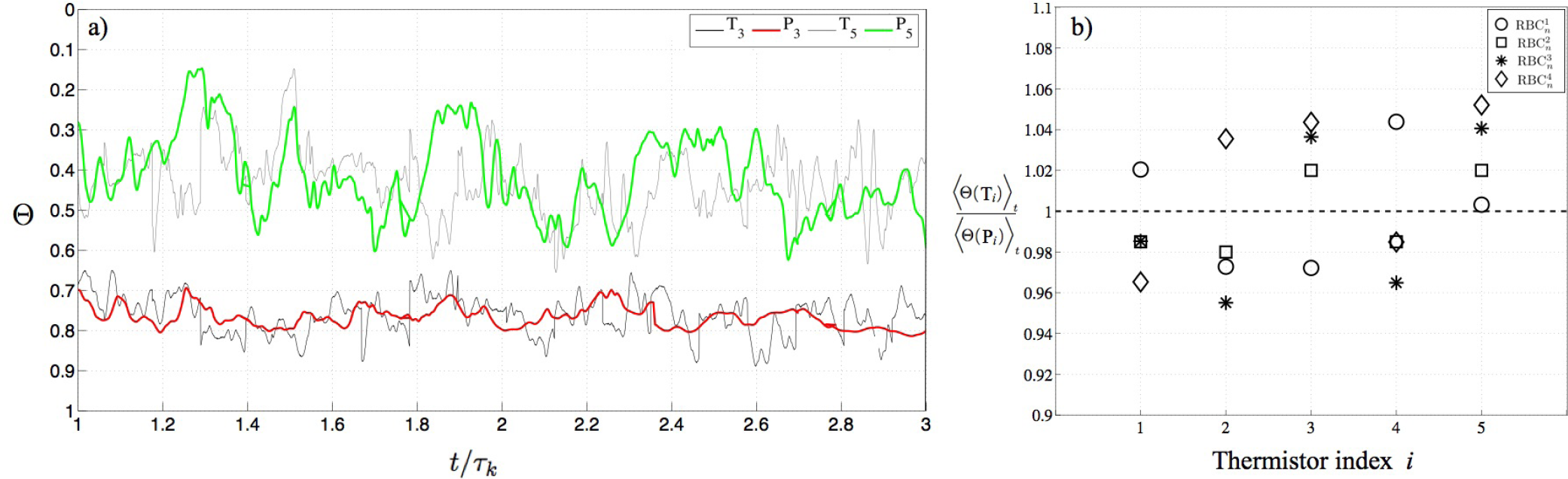


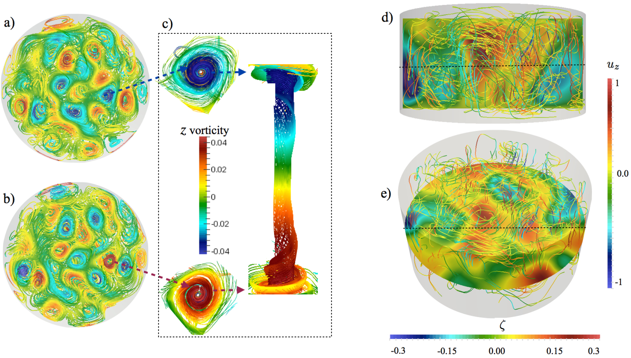


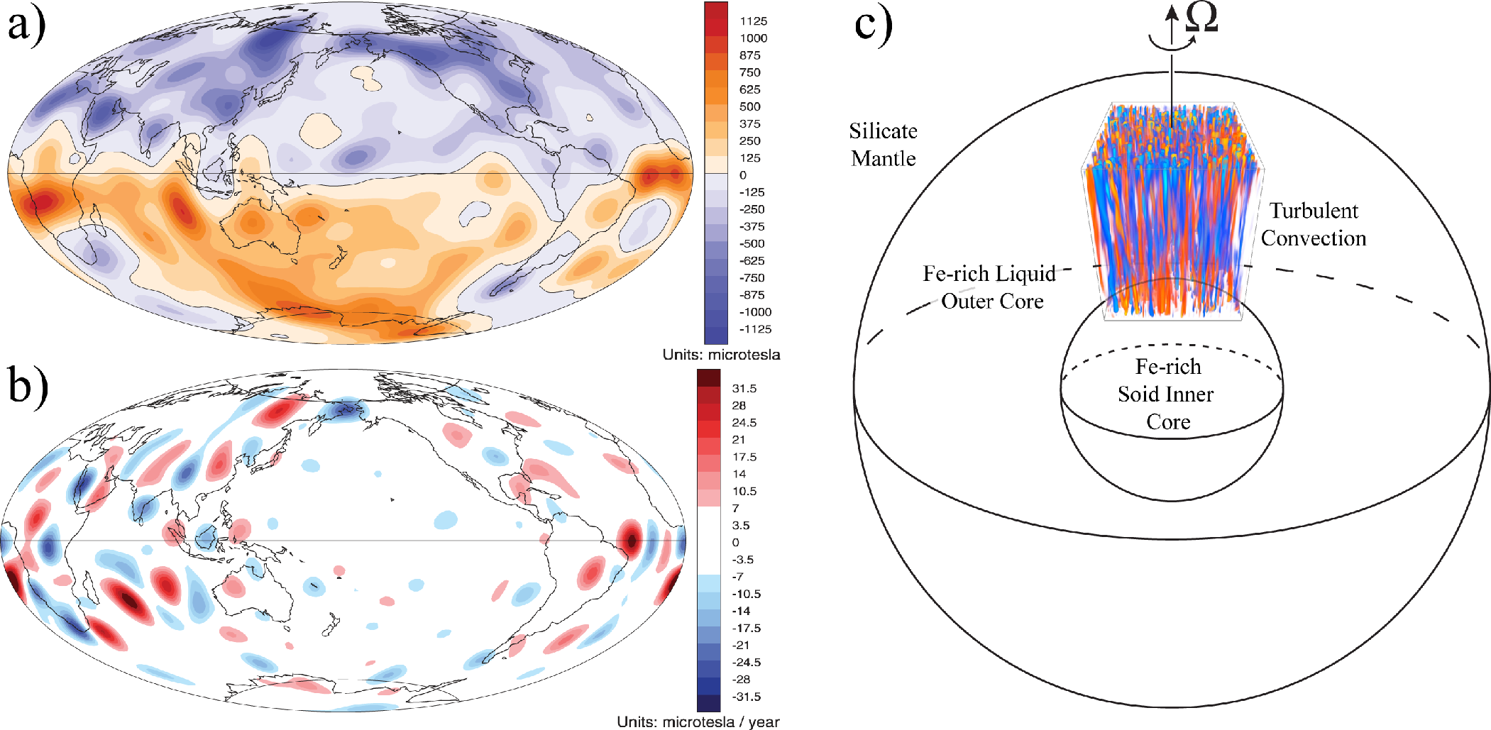
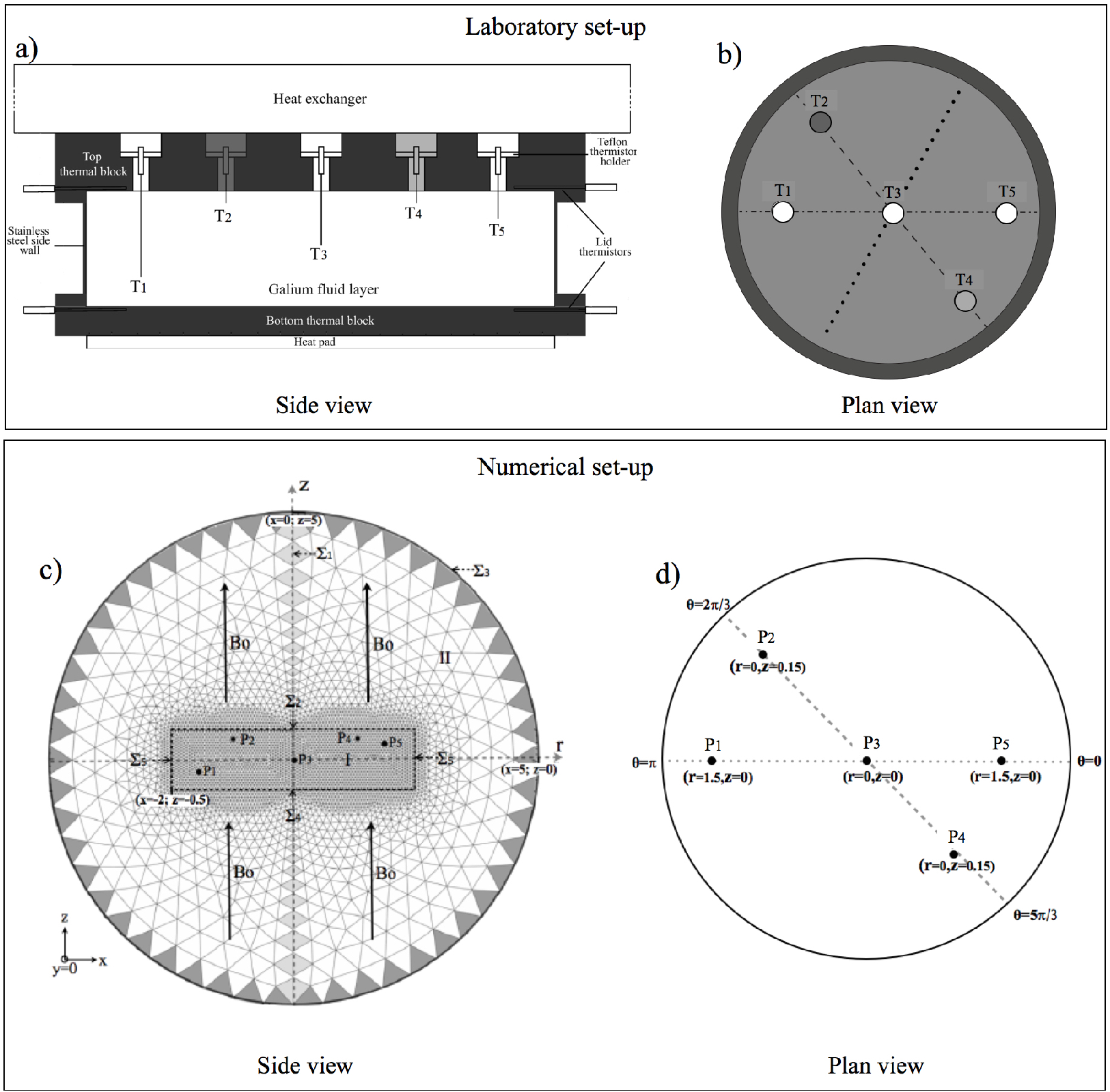
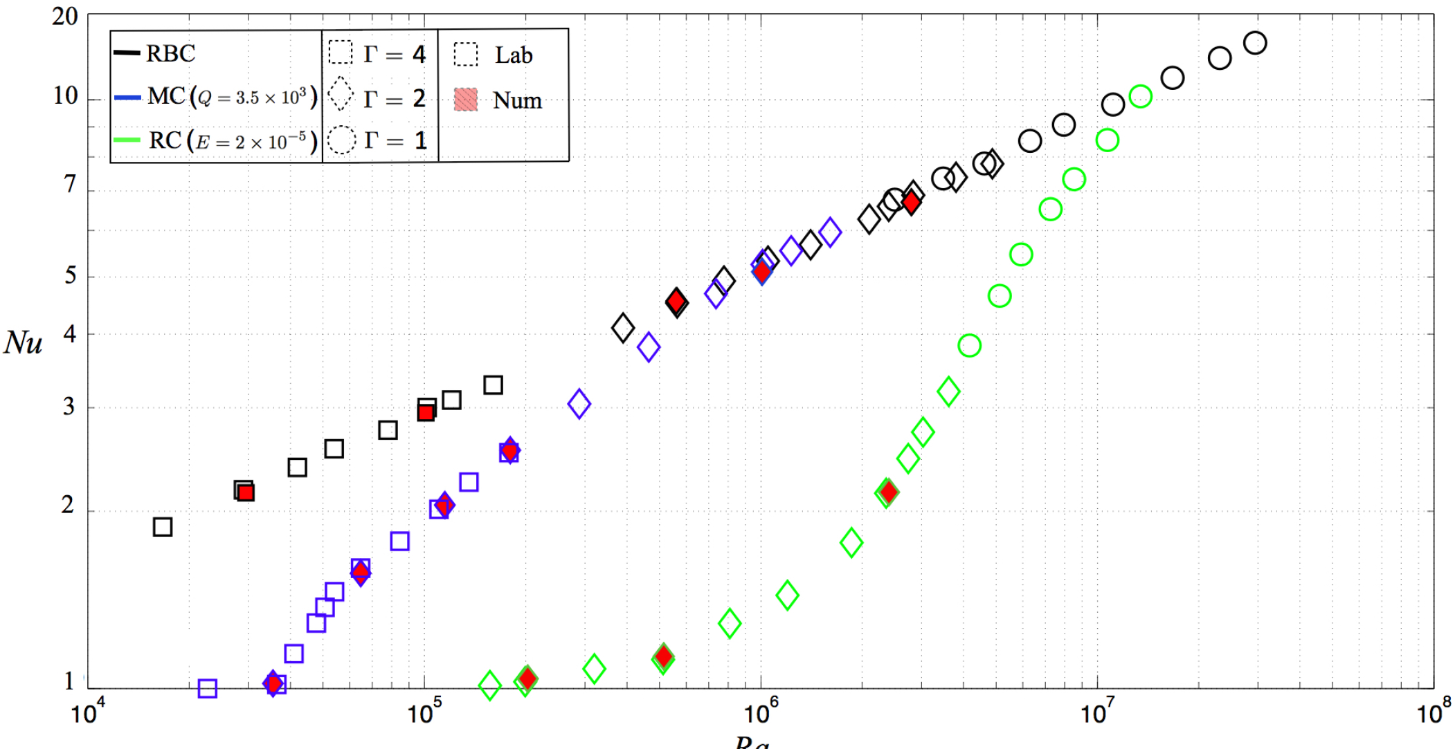
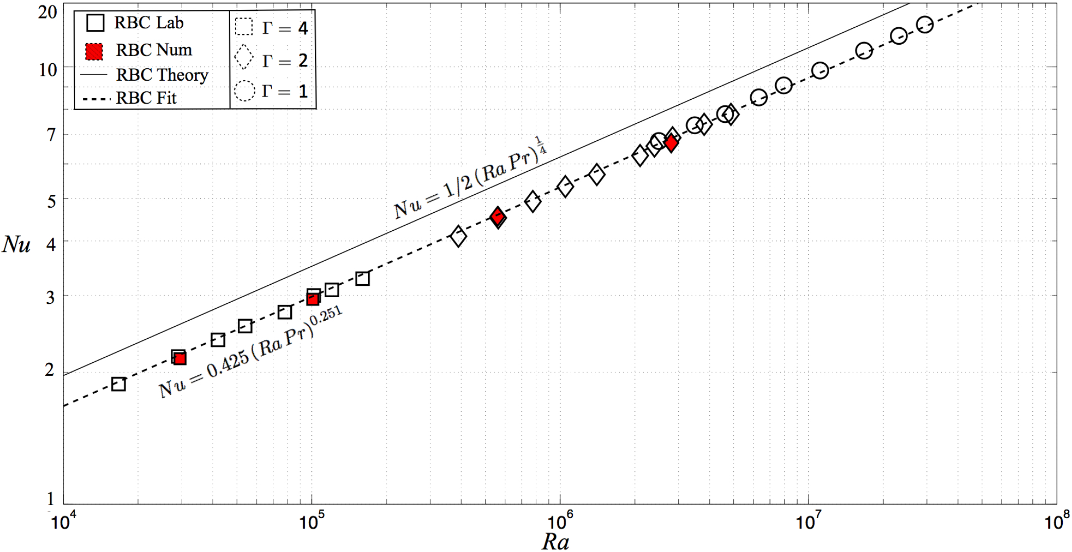
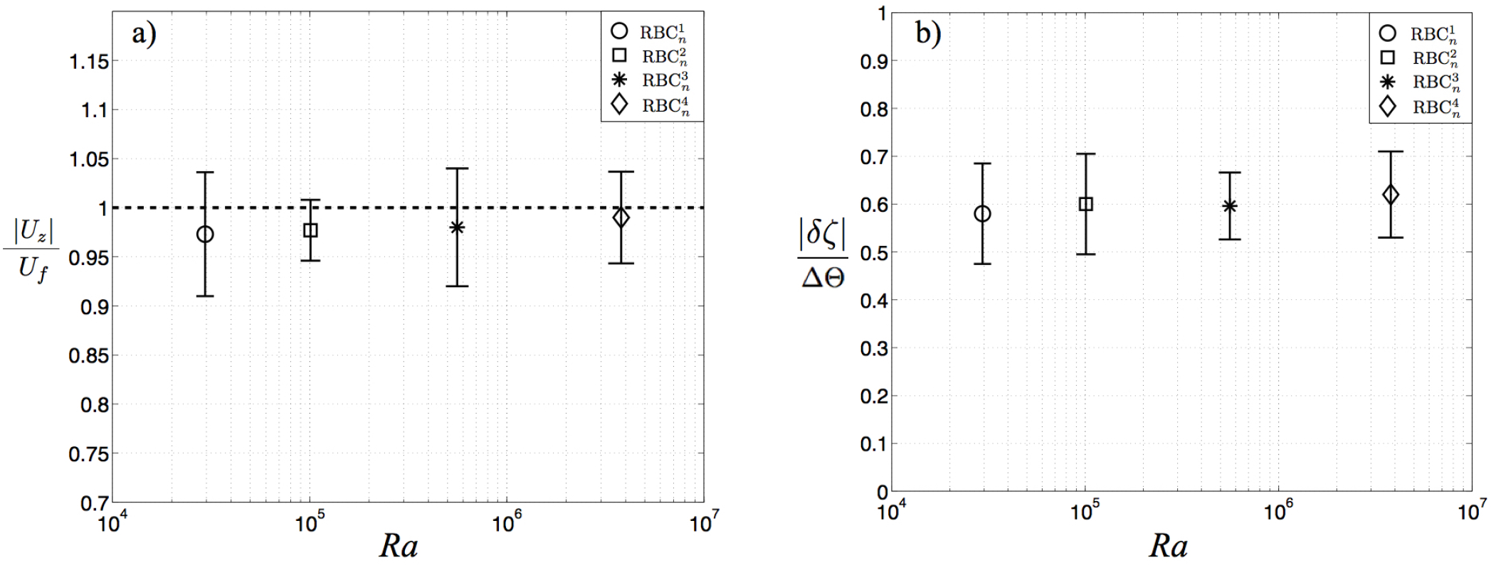
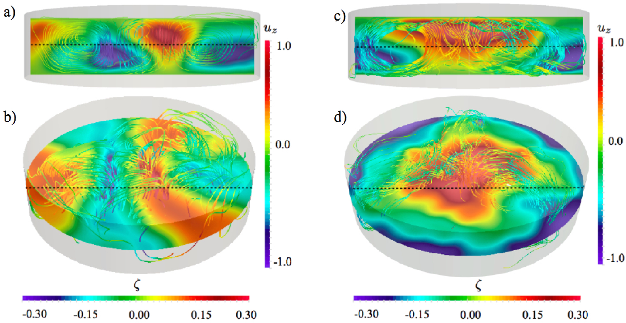
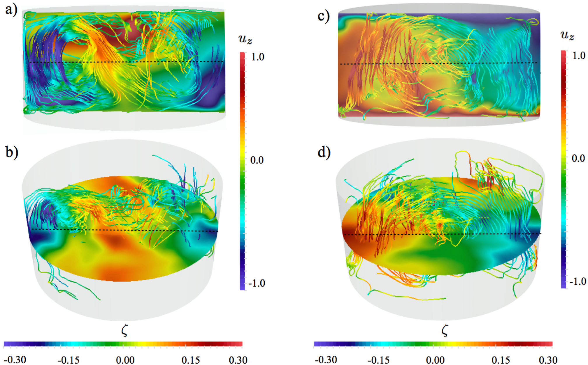
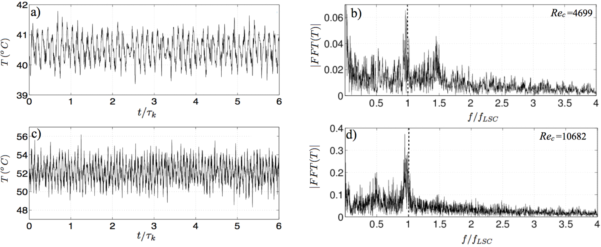
| Property | Value |
|---|---|
| Mass density | ρ = 6.1 × 10³ kg/m3 |
| Thermal expansivity | α = 1.3 × 10⁻⁴ K−1 |
| Specific heat | Cp = 398 J/(kg K) |
| Thermal conductivity | K = 31 W/(m K) |
| Electrical conductivity | σ = 3.9 × 10⁶ (Ohm m)−1 |
| Magnetic diffusivity | η = 0.2 m2/s |
| Thermal diffusivity | κ = 1.3 × 10⁻⁵ m2/s |
| kinematic viscosity | ν = 3.2 × 10⁻⁷ m2/s |
| System | Pr | Pm | Ra | Q | E |
|---|---|---|---|---|---|
| Laboratory | ≃0.025 | 1.5 × 10⁻⁶ | 104 – 3 × 10⁷ | ≃3.5 × 10³ | ≃2 × 10⁻⁵ |
| SFEMaNS-T | 0.025 | 10−4 | 3 × 10⁴–2 × 10⁶ | 3.5 × 10³ | 2 × 10⁻⁵ |
| Earth’s core | ∼0.01 | ∼10−5 | 1020–1030 | ∼1015 | ∼10−15 |
| System | Rec | P ec | Rmc | Nc | Roc |
| Laboratory | 800 – 3.5 × 10⁴ | 20–880 | 10−3–0.05 | 30–2300 | 0.05–0.5 |
| SFEMaNS-T | 1100–10, 000 | 28–225 | 0.1–0.9 | 0.4–30 | 0.05–0.20 |
| Earth’s core | ∼108 | ∼106 | ∼102 | ∼107 | ∼10−7 |
| Case | H [cm] | P [W] | ΔT [°C] | Γ | Pr | Rec | Ra | Nu | |
|---|---|---|---|---|---|---|---|---|---|
| 5 | 35 | 36.7 | 0.73 | 3.92 | 0.0255 | 733 | 1.37 × 10⁴ | 1.71 | |
| 5 | 51 | 37.2 | 0.97 | 3.92 | 0.0255 | 809 | 1.67 × 10⁴ | 1.80 | |
| 5 | 75 | 38.1 | 1.29 | 3.92 | 0.0254 | 1068 | 2.90 × 10⁴ | 2.10 | |
| 5 | 100 | 38.9 | 1.69 | 3.92 | 0.0254 | 1174 | 3.42 × 10⁴ | 2.18 | |
| 5 | 151 | 37.7 | 2.51 | 3.92 | 0.0255 | 1268 | 4.10 × 10⁴ | 2.29 | |
| 5 | 248 | 40.5 | 3.89 | 3.92 | 0.0251 | 1762 | 7.80 × 10⁴ | 2.67 | |
| 5 | 346 | 43.2 | 5.19 | 3.92 | 0.0248 | 2028 | 1.02 × 10⁵ | 2.92 | |
| 10 | 68 | 37.7 | 1.60 | 1.87 | 0.0259 | 3880 | 3.90 × 10⁵ | 4.10 | |
| 10 | 148 | 40.5 | 3.17 | 1.87 | 0.0259 | 4650 | 5.60 × 10⁵ | 4.51 | |
| 10 | 214 | 42.7 | 4.30 | 1.87 | 0.0258 | 5488 | 7.77 × 10⁵ | 4.92 | |
| 10 | 303 | 45.6 | 5.72 | 1.87 | 0.0258 | 6226 | 1.00 × 10⁶ | 5.32 | |
| 10 | 399 | 45.1 | 7.20 | 1.87 | 0.0259 | 7352 | 1.40 × 10⁶ | 5.67 | |
| 10 | 496 | 47.1 | 8.53 | 1.87 | 0.0257 | 8844 | 2.01 × 10⁶ | 6.27 | |
| 10 | 597 | 48.5 | 9.74 | 1.87 | 0.0254 | 9720 | 2.40 × 10⁶ | 6.60 | |
| 10 | 744 | 52.1 | 11.50 | 1.87 | 0.0247 | 10704 | 2.83 × 10⁶ | 6.88 | |
| 10 | 1075 | 51.7 | 15.41 | 1.87 | 0.0248 | 12378 | 3.80 × 10⁶ | 7.46 | |
| 10 | 1480 | 62.0 | 19.70 | 1.87 | 0.0237 | 14349 | 4.88 × 10⁶ | 7.80 | |
| Case | np | nS | nF | Γ | Rec | Ra | Nu | |Uz|/Uf | |δζ|/ΔΘ |
|---|---|---|---|---|---|---|---|---|---|
| 18,653 | 2 | 32 | 4 | 1086 | 2.95 × 10⁴ | 2.15 | 0.95 | 0.57 | |
| 35,325 | 4 | 64 | 4 | 2010 | 1.01 × 10⁵ | 2.94 | 0.96 | 0.60 | |
| 37,632 | 4 | 128 | 2 | 4732 | 5.60 × 10⁵ | 4.55 | 0.96 | 0.60 | |
| 46,565 | 4 | 200 | 2 | 10,639 | 2.83 × 10⁶ | 6.70 | 0.97 | 0.63 |
| Case | Bo | H | P | T | ΔT | Γ | Pr | Q | N | Rec | Ra | Nu |
|---|---|---|---|---|---|---|---|---|---|---|---|---|
| 26.0 | 5 | 20.9 | 36.7 | 0.75 | 3.92 | 0.0256 | 3.48 × 10³ | 3.67 | 948 | 2.30 × 10⁴ | 0.99 | |
| 26.0 | 5 | 30.1 | 37.2 | 1.21 | 3.92 | 0.0255 | 3.50 × 10³ | 2.93 | 1195 | 3.64 × 10⁴ | 1.01 | |
| 26.0 | 5 | 51.2 | 37.8 | 1.70 | 3.92 | 0.0255 | 3.53 × 10³ | 2.76 | 1280 | 4.18 × 10⁴ | 1.14 | |
| 26.0 | 5 | 59.8 | 38.2 | 1.91 | 3.92 | 0.0254 | 3.55 × 10³ | 2.59 | 1371 | 4.78 × 10⁴ | 1.37 | |
| 26.0 | 5 | 70.2 | 38.5 | 2.01 | 3.92 | 0.0254 | 3.56 × 10³ | 2.44 | 1460 | 5.42 × 10⁴ | 1.43 | |
| 26.0 | 5 | 75.7 | 38.7 | 2.24 | 3.92 | 0.0253 | 3.57 × 10³ | 2.23 | 1597 | 6.46 × 10⁴ | 1.59 | |
| 26.0 | 5 | 125.1 | 40.36 | 3.21 | 3.92 | 0.0252 | 3.59 × 10³ | 1.96 | 1831 | 8.45 × 10⁴ | 1.77 | |
| 26.0 | 5 | 200.7 | 42.5 | 4.41 | 3.92 | 0.0251 | 3.62 × 10³ | 1.72 | 2102 | 1.11 × 10⁵ | 2.00 | |
| 26.0 | 5 | 299.7 | 42.75 | 5.85 | 3.92 | 0.0251 | 3.63 × 10³ | 1.56 | 2319 | 1.35 × 10⁵ | 2.23 | |
| 26.0 | 5 | 346 | 43.2 | 5.19 | 3.92 | 0.0248 | 3.59 × 10³ | 1.29 | 2775 | 1.91 × 10⁵ | 2.59 | |
| 13.0 | 10 | 32.3 | 37.3 | 1.00 | 1.87 | 0.0254 | 3.54 × 10³ | 1.04 | 3414 | 2.96 × 10⁵ | 3.04 | |
| 13.0 | 10 | 60.5 | 38.7 | 1.60 | 1.87 | 0.0253 | 3.54 × 10³ | 0.82 | 4319 | 4.72 × 10⁵ | 3.80 | |
| 13.0 | 10 | 111.8 | 41.1 | 2.56 | 1.87 | 0.0251 | 3.60 × 10³ | 0.66 | 5470 | 7.51 × 10⁵ | 4.68 | |
| 13.0 | 10 | 169.3 | 43.7 | 3.72 | 1.87 | 0.0248 | 3.64 × 10³ | 0.56 | 6444 | 1.03 × 10⁶ | 5.25 | |
| 13.0 | 10 | 217.7 | 45.8 | 4.25 | 1.87 | 0.0247 | 3.67 × 10³ | 0.52 | 7085 | 1.24 × 10⁶ | 5.54 | |
| 13.0 | 10 | 307.4 | 48.1 | 5.56 | 1.87 | 0.0245 | 3.71 × 10³ | 0.33 | 11314 | 1.60 × 10⁶ | 5.95 | |
| Case | np | nS | nF | Γ | N | Rec | Ra | Nu | |Uz|/Uf | |δζ|/ΔΘ |
|---|---|---|---|---|---|---|---|---|---|---|
| 12,854 | 1 | 32 | 4 | 2.94 | 1190 | 3.54 × 10⁴ | 1.01 | – | – | |
| 12,854 | 1 | 32 | 4 | 2.17 | 1609 | 6.47 × 10⁴ | 1.63 | 0.40 | 0.38 | |
| 37,632 | 4 | 64 | 4 | 1.63 | 2145 | 1.15 × 10⁵ | 2.05 | 0.88 | 0.57 | |
| 37,632 | 4 | 64 | 4 | 1.30 | 2683 | 1.80 × 10⁵ | 2.54 | 0.92 | 0.62 | |
| 46,5650 | 4 | 128 | 2 | 0.55 | 6324 | 1.00 × 10⁶ | 5.15 | 0.93 | 0.63 |
| Case | P [W] | ΔT [°C] | Pr | E | Roc | Ra | Nu | |
|---|---|---|---|---|---|---|---|---|
| 10.4 | 36.5 | 0.81 | 0.0256 | 2.08 × 10⁻⁵ | 0.050 | 1.56 × 10⁵ | 1.01 | |
| 20.2 | 37.2 | 1.20 | 0.0255 | 2.06 × 10⁻⁵ | 0.056 | 1.92 × 10⁵ | 1.02 | |
| 31.1 | 38.1 | 2.70 | 0.0255 | 2.05 × 10⁻⁵ | 0.076 | 3.50 × 10⁵ | 1.08 | |
| 40.0 | 38.5 | 3.30 | 0.0255 | 2.05 × 10⁻⁵ | 0.092 | 5.11 × 10⁵ | 1.12 | |
| 59.8 | 39.6 | 4.50 | 0.0254 | 2.04 × 10⁻⁵ | 0.115 | 8.08 × 10⁵ | 1.29 | |
| 79.8 | 41.4 | 5.97 | 0.0253 | 2.04 × 10⁻⁵ | 0.140 | 1.20 × 10⁶ | 1.44 | |
| 150.3 | 48.2 | 10.6 | 0.0242 | 2.01 × 10⁻⁵ | 0.176 | 1.86 × 10⁶ | 1.77 | |
| 206.1 | 48.7 | 12.41 | 0.0242 | 2.01 × 10⁻⁵ | 0.198 | 2.35 × 10⁶ | 2.10 | |
| 302.5 | 51.4 | 15.44 | 0.0240 | 1.96 × 10⁻⁵ | 0.209 | 2.74 × 10⁶ | 2.46 | |
| 399.4 | 48.6 | 17.31 | 0.0242 | 1.97 × 10⁻⁵ | 0.220 | 3.03 × 10⁶ | 2.72 | |
| 496.5 | 46.8 | 19.00 | 0.0244 | 1.99 × 10⁻⁵ | 0.242 | 3.61 × 10⁶ | 3.20 | |
| Case | np | nS | nF | Γ | Roc | Ra | Nu | |Uz|/Uf | |δζ|/ΔΘ |
|---|---|---|---|---|---|---|---|---|---|
| 37,632 | 4 | 64 | 2 | 0.045 | 1.21 × 10⁵ | 1.01 | – | – | |
| 46,565 | 4 | 64 | 2 | 0.104 | 6.47 × 10⁵ | 1.06 | 0.40 | 0.38 | |
| 46,565 | 4 | 128 | 2 | 0.183 | 2.00 × 10⁶ | 2.05 | 0.88 | 0.55 |
© 2015 by the authors; licensee MDPI, Basel, Switzerland This article is an open access article distributed under the terms and conditions of the Creative Commons Attribution license (http://creativecommons.org/licenses/by/4.0/).
Share and Cite
Ribeiro, A.; Fabre, G.; Guermond, J.-L.; Aurnou, J.M. Canonical Models of Geophysical and Astrophysical Flows: Turbulent Convection Experiments in Liquid Metals. Metals 2015, 5, 289-335. https://doi.org/10.3390/met5010289
Ribeiro A, Fabre G, Guermond J-L, Aurnou JM. Canonical Models of Geophysical and Astrophysical Flows: Turbulent Convection Experiments in Liquid Metals. Metals. 2015; 5(1):289-335. https://doi.org/10.3390/met5010289
Chicago/Turabian StyleRibeiro, Adolfo, Guillaume Fabre, Jean-Luc Guermond, and Jonathan M. Aurnou. 2015. "Canonical Models of Geophysical and Astrophysical Flows: Turbulent Convection Experiments in Liquid Metals" Metals 5, no. 1: 289-335. https://doi.org/10.3390/met5010289