Three-Dimensional Lattice Boltzmann Modeling of Dendritic Solidification under Forced and Natural Convection


Abstract
:1. Introduction
2. Model Description
3. Results and Discussion
3.1. Validation
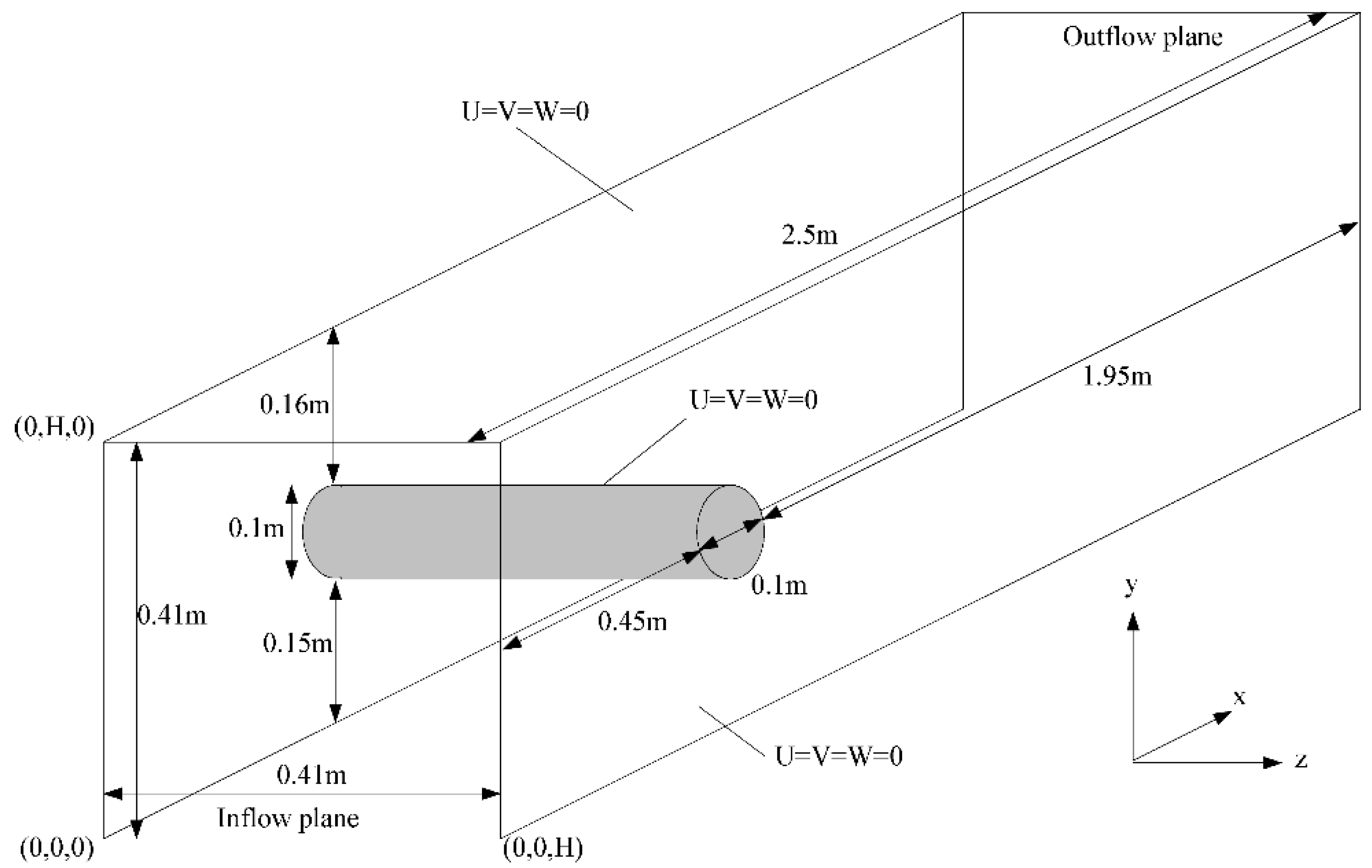
3.1.1. Fluid Flow
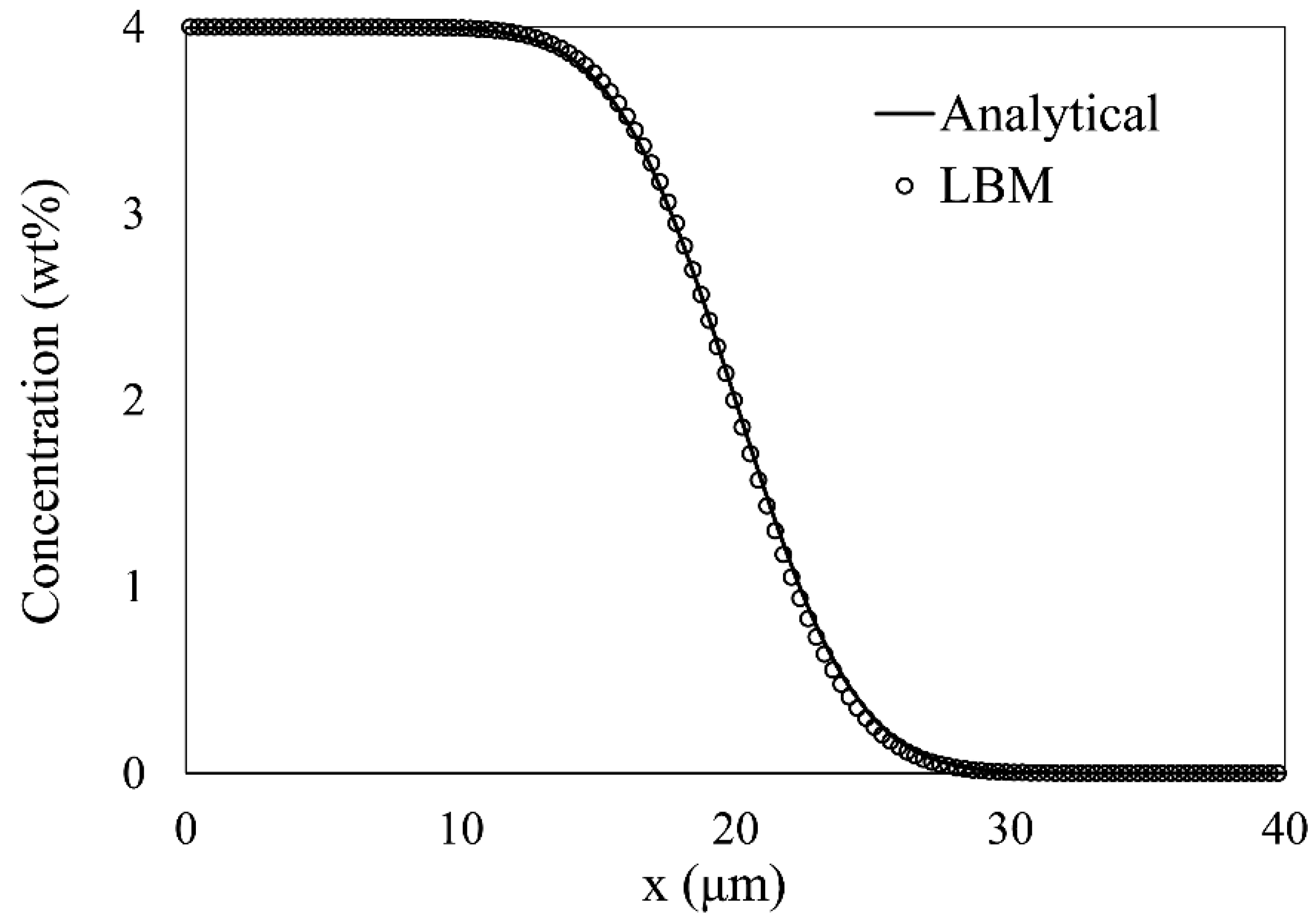
3.1.2. Solute Transport
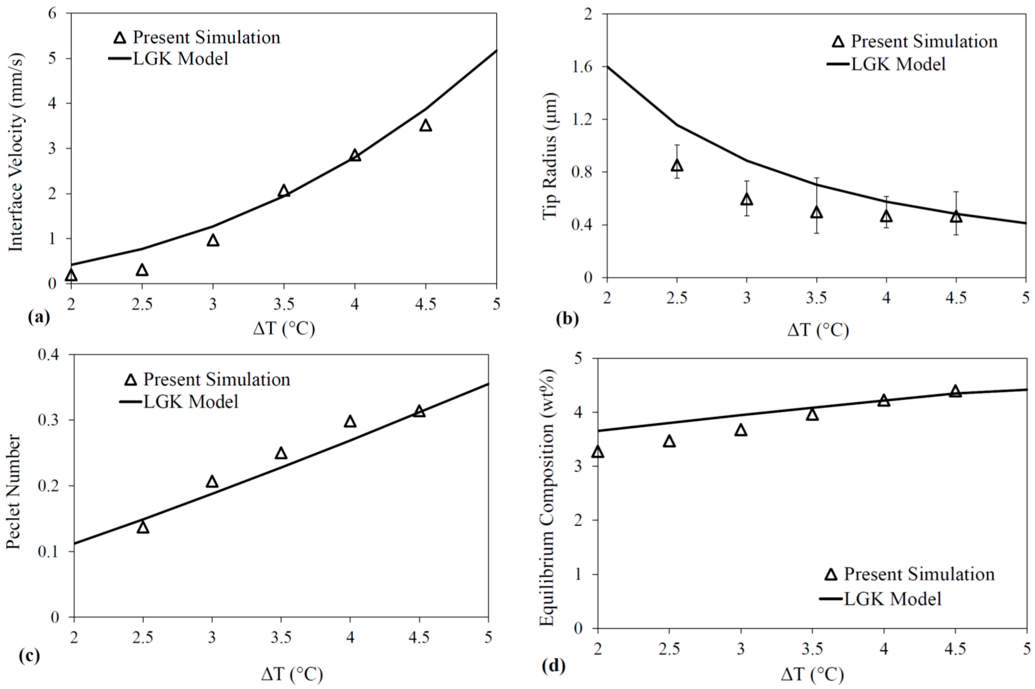
3.1.3. Dendrite Growth
3.2. Dendrite Growth under Melt Convection
3.2.1. Kinetics of Growth under Forced Convection
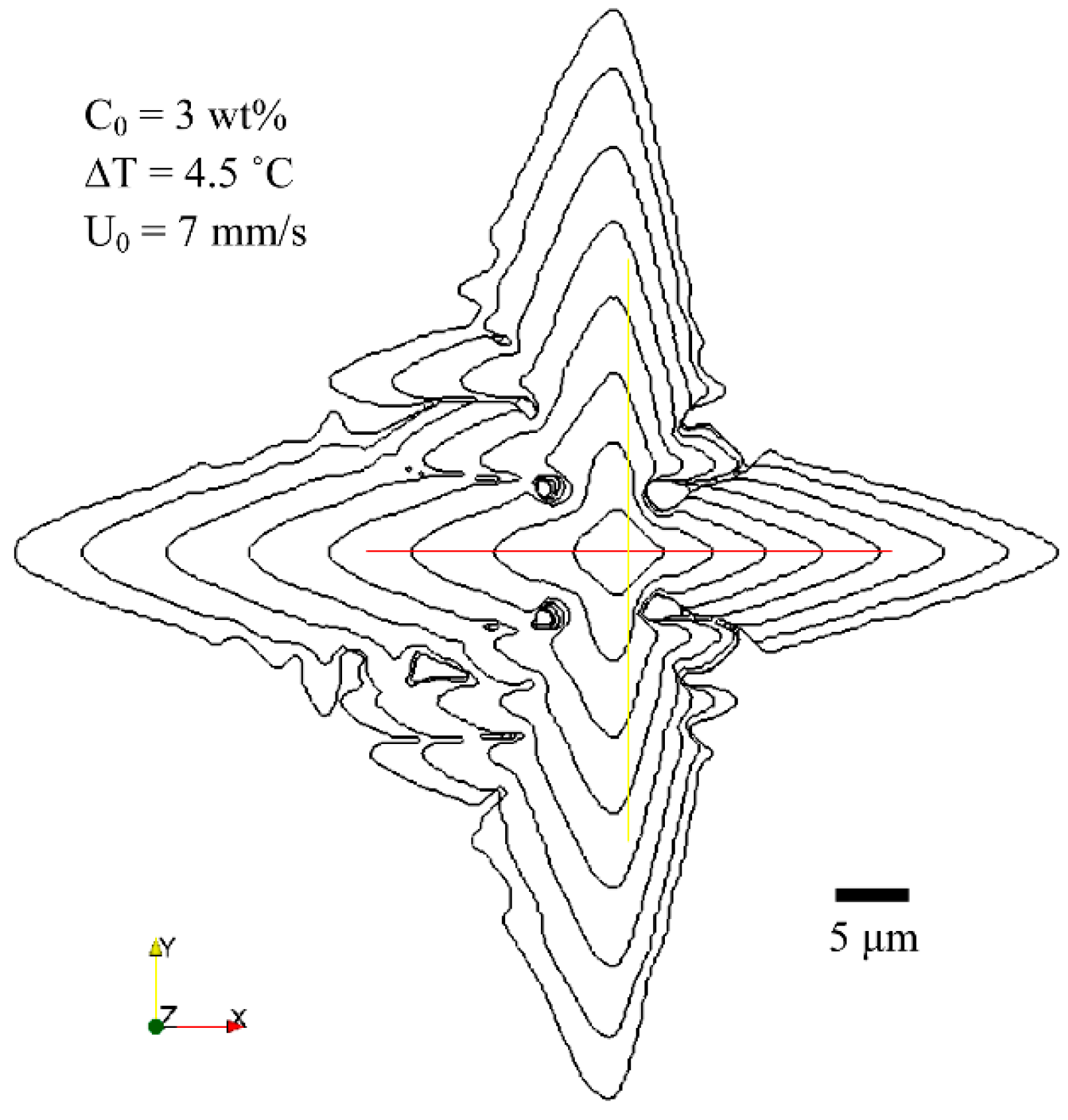
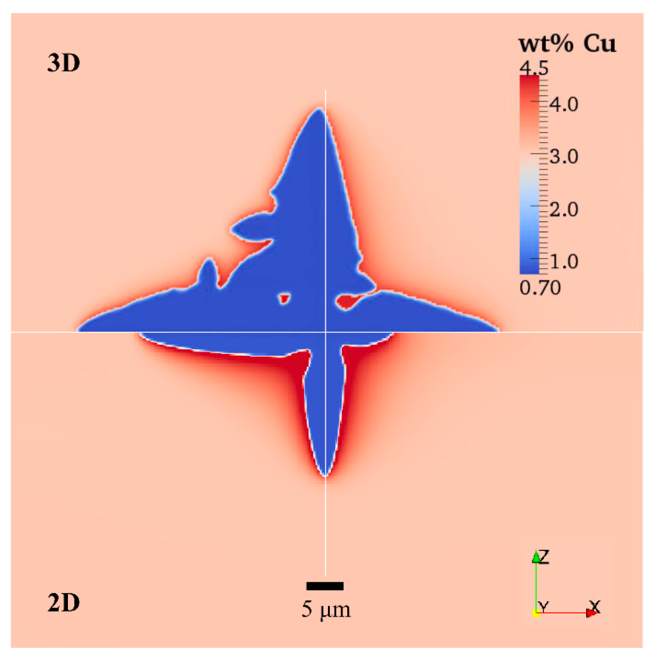
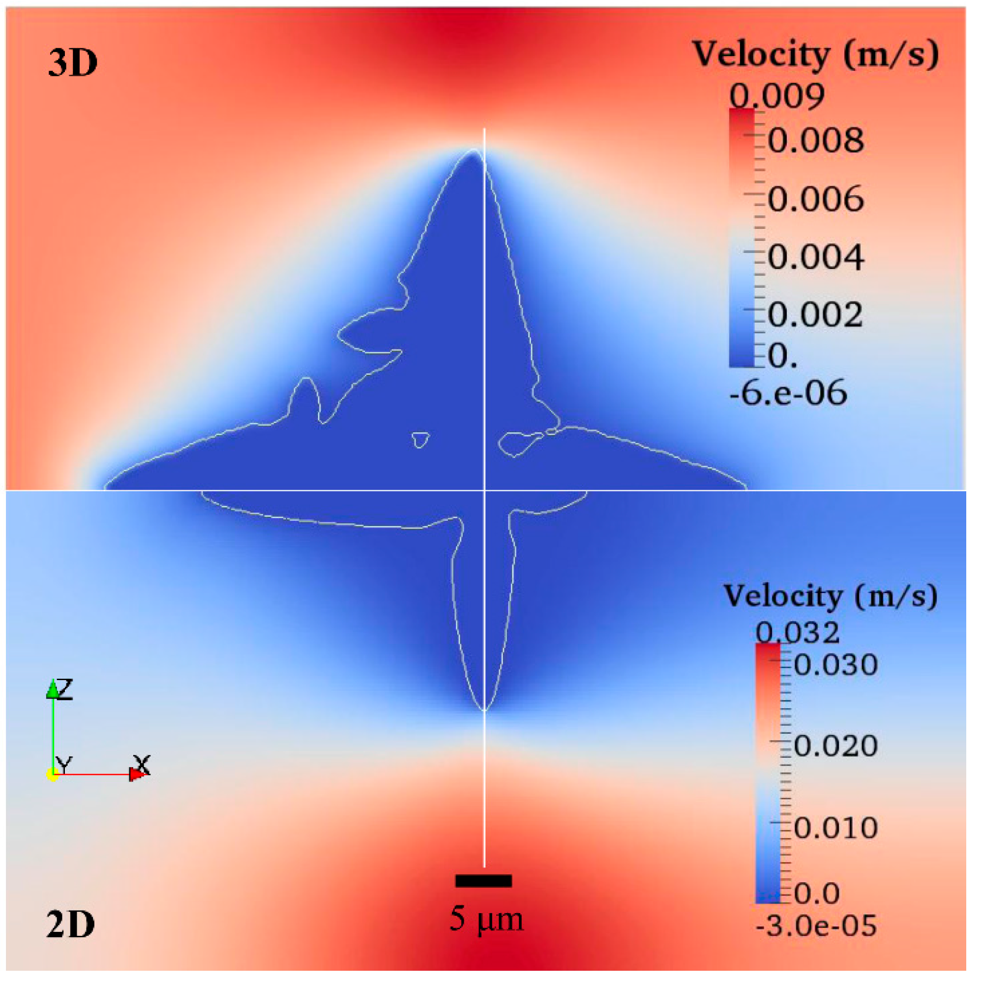
3.2.2. Comparison of 2D and 3D Simulations
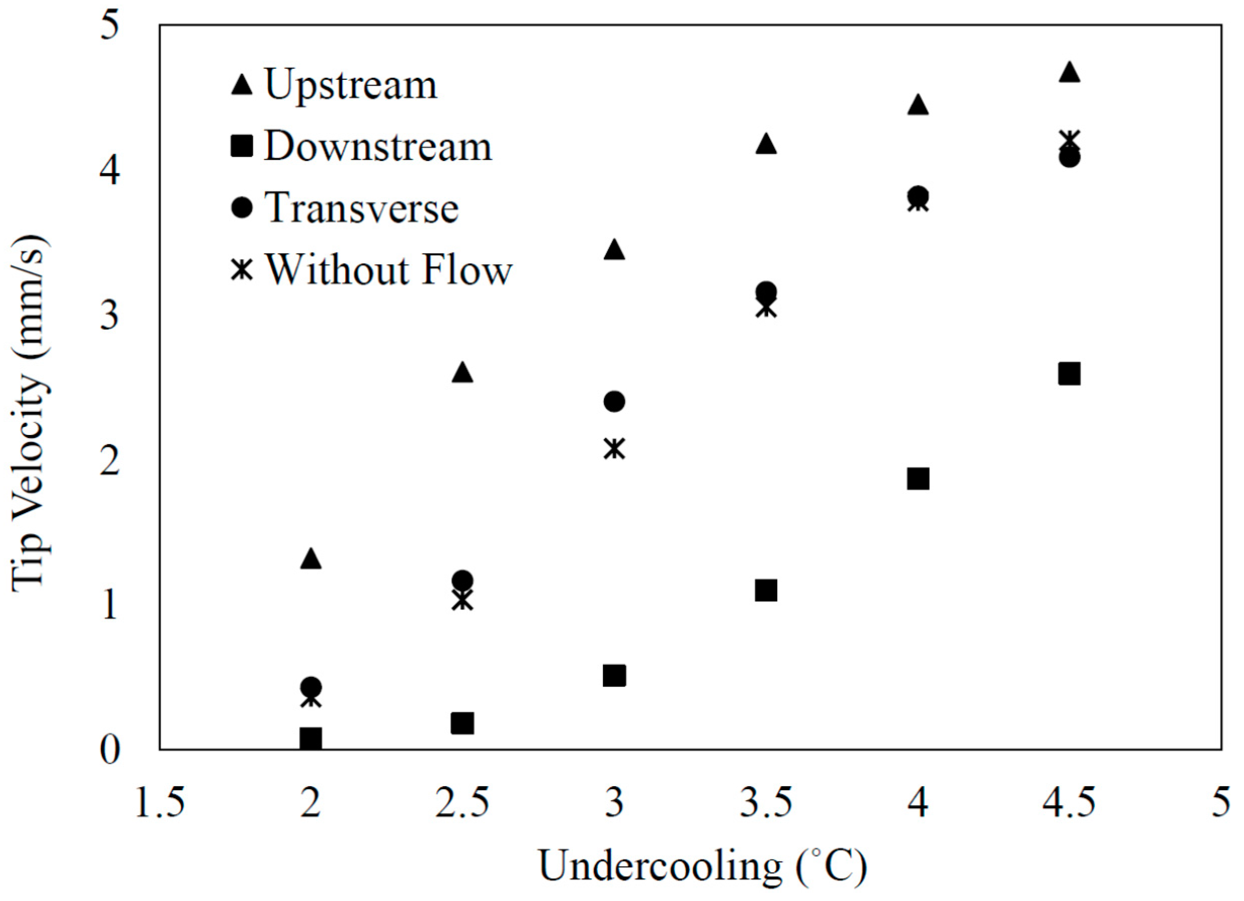
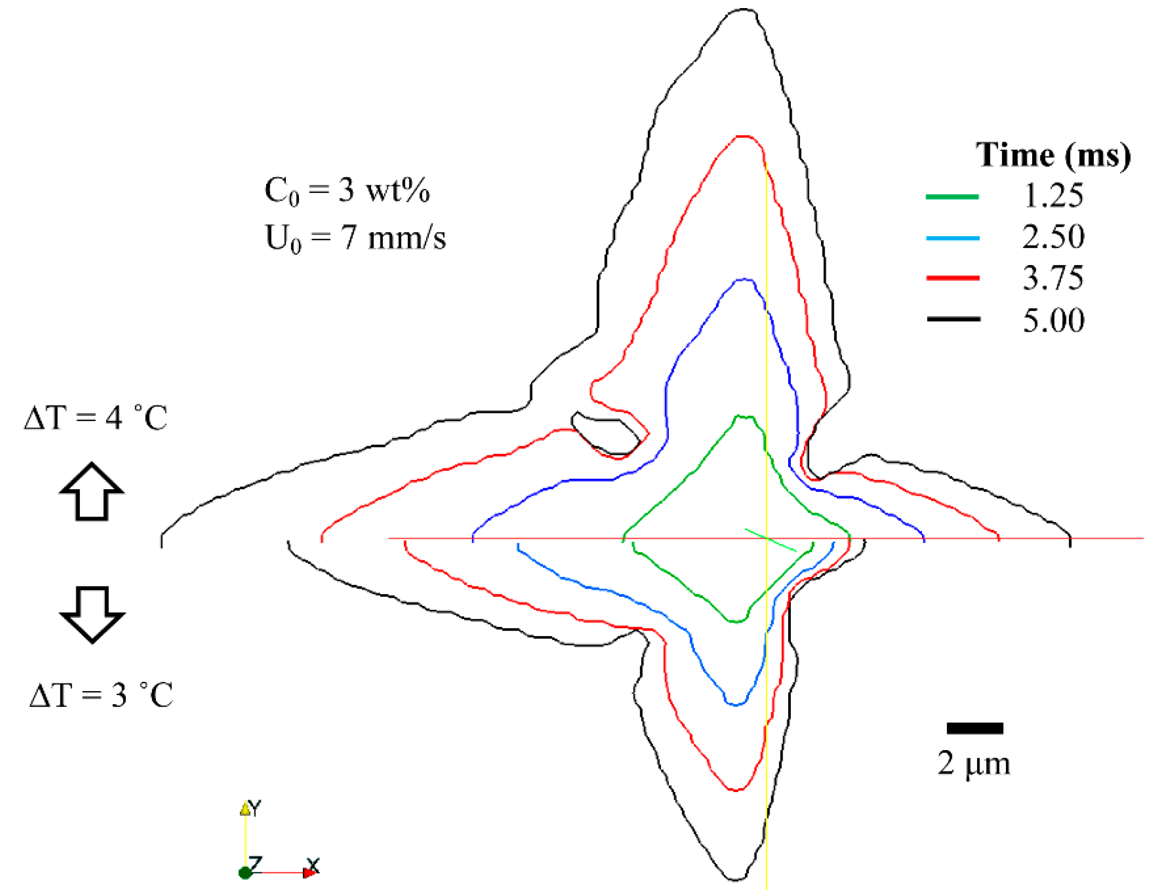
3.2.3. Effect of Melt Flow and Undercooling Strength
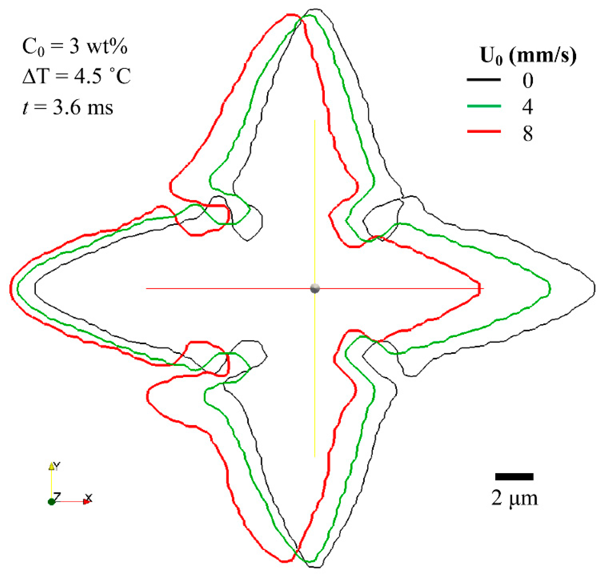
3.2.4. Effect of Inlet Velocity
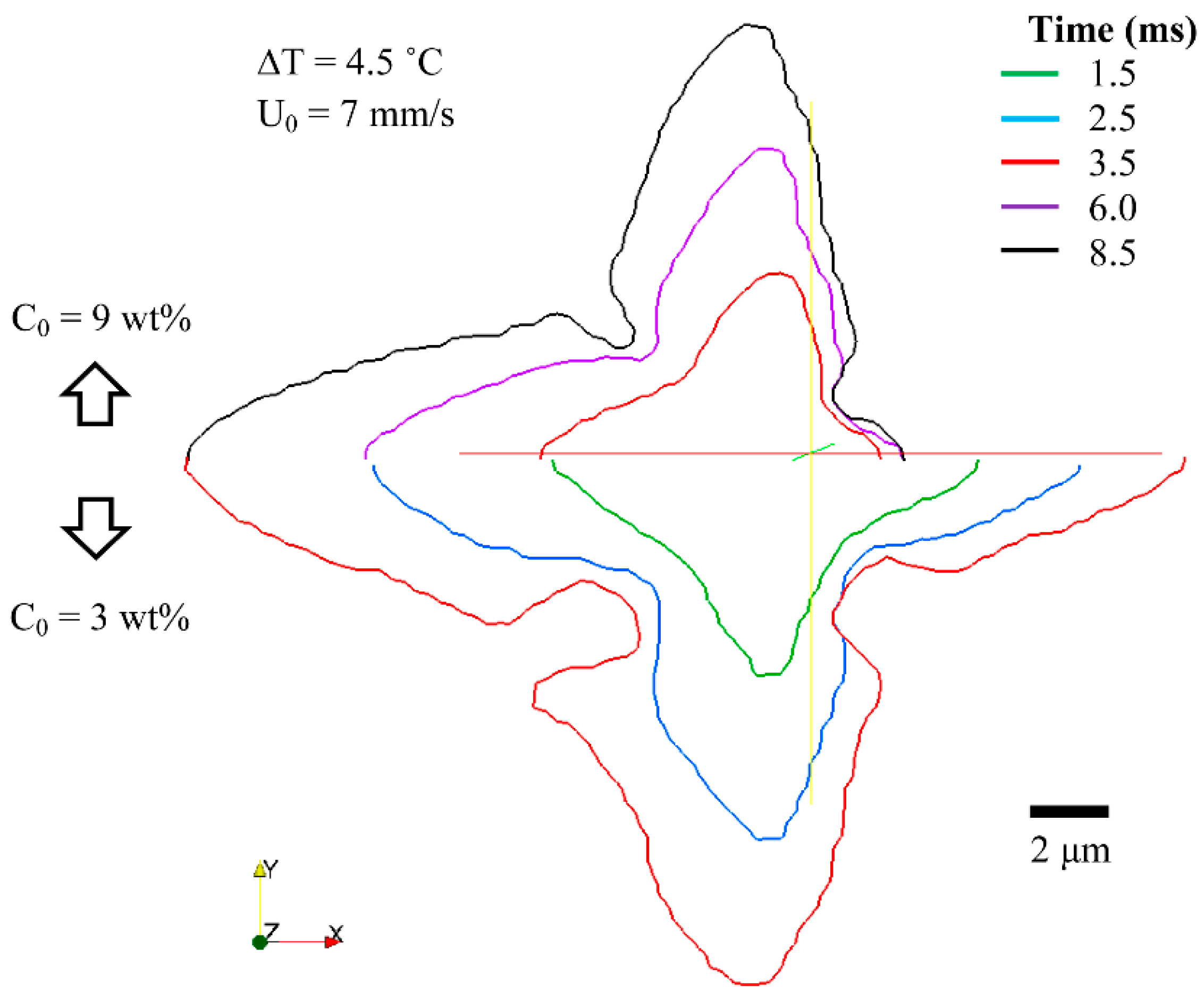
3.2.5. Effect of Alloy Composition
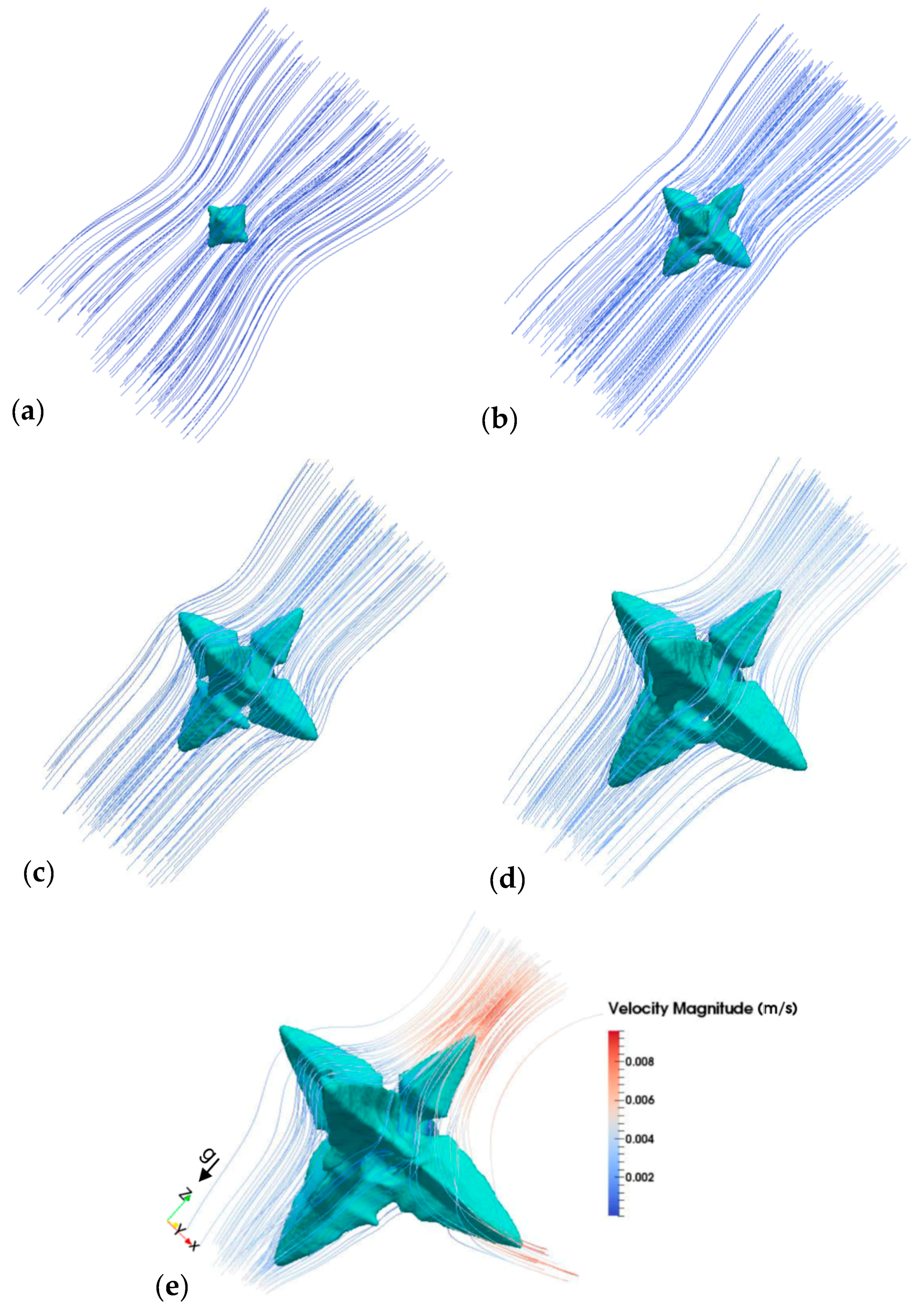
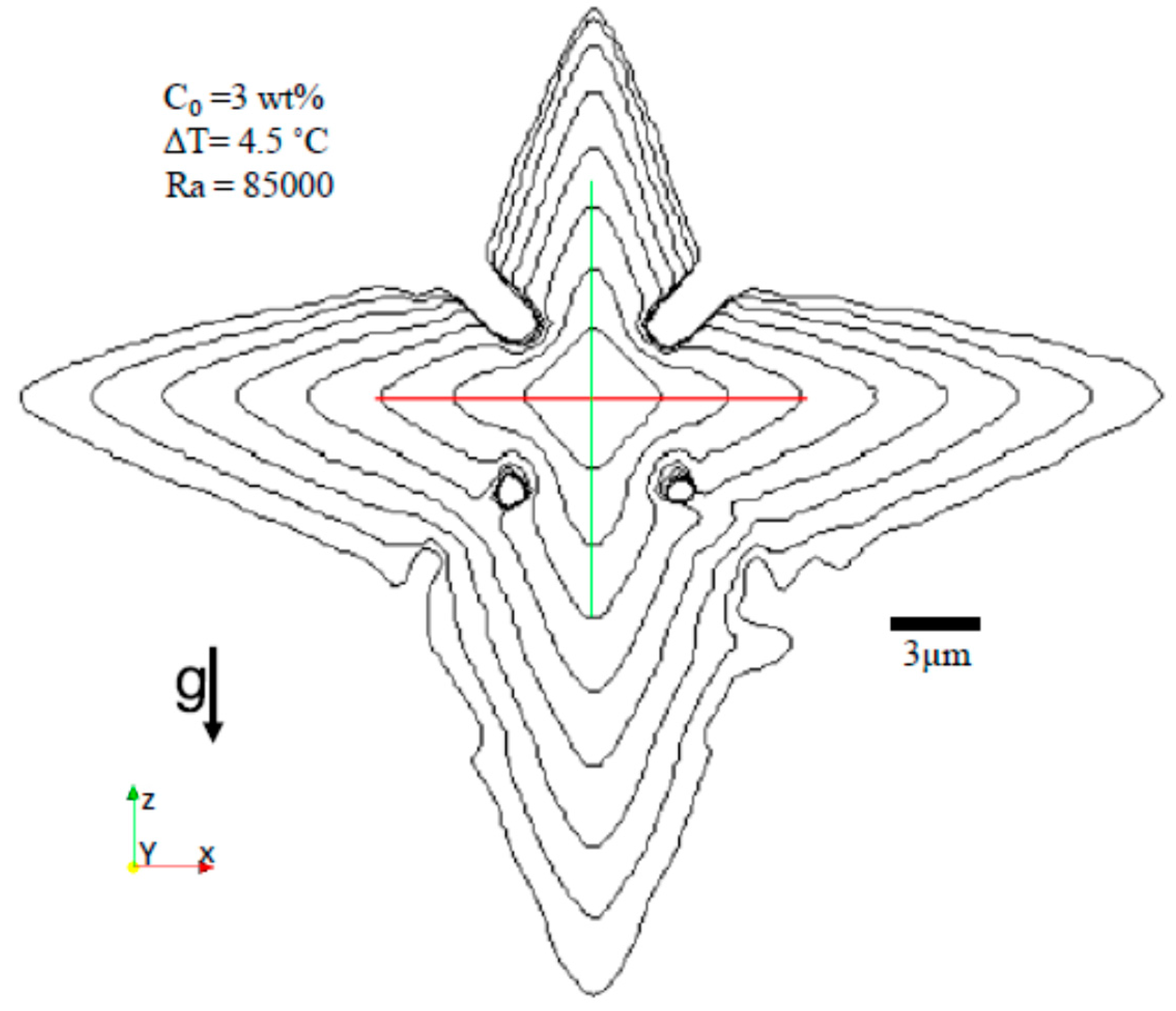
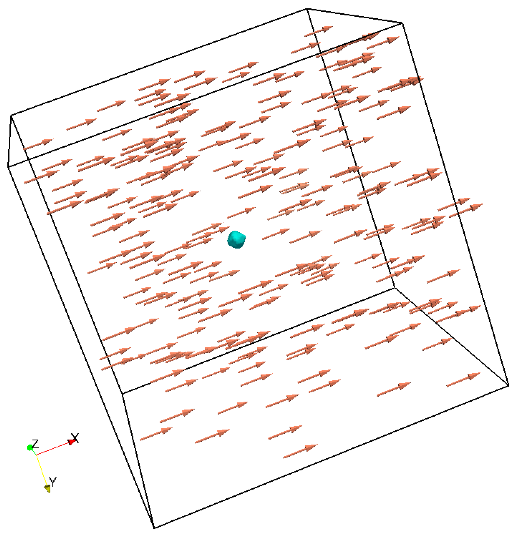
3.2.6. Effect of Natural Convection
4. Conclusions
Acknowledgments
Author Contributions
Conflicts of Interest
References
- Boettinger, W.J.; Warren, J.A.; Beckermann, C.; Karma, A. Phase-field simulation of solidification. Annu. Rev. Mater. Res. 2002, 32, 163–194. [Google Scholar] [CrossRef]
- Badillo, A.; Beckermann, C. Phase-field simulation of the columnar-to-equiaxed transition in alloy solidification. Acta Mater. 2006, 54, 2015–2026. [Google Scholar] [CrossRef]
- Hoyt, J.J.; Asta, M.; Karma, A. Atomistic and continuum modeling of dendritic solidification. Mater. Sci. Eng. R 2003, 41, 121–163. [Google Scholar] [CrossRef]
- Karma, A.; Rappel, W.J. Quantitative phase-field modeling of dendritic growth in two and three dimensions. Phys. Rev. E 1998, 57, 4323. [Google Scholar] [CrossRef]
- Provatas, N.; Goldenfeld, N.; Dantzig, J.A. Adaptive mesh refinement computation of solidification microstructures using dynamic data structures. J. Comput. Phys. 1999, 148, 265–290. [Google Scholar] [CrossRef]
- Gibou, F.; Fedkiw, R.P.; Cheng, L.-T.; Kang, M. A second-order-accurate symmetric discretization of the Poisson equation on irregular domains. J. Comput. Phys. 2002, 176, 205–227. [Google Scholar] [CrossRef]
- Gibou, F.; Fedkiw, R.; Caflisch, R.; Osher, S. A level set approach for the numerical simulation of dendritic growth. J. Sci. Comput. 2003, 19, 183–199. [Google Scholar] [CrossRef]
- Kim, Y.-T.; Goldenfeld, N.; Dantzig, J.A. Computation of dendritic microstructures using a level set method. Phys. Rev. E 2000, 62, 2471–2474. [Google Scholar] [CrossRef]
- Osher, S.; Fedkiw, R.P. Level set methods: An overview and some recent results. J. Comput. Phys. 2001, 169, 463–502. [Google Scholar] [CrossRef]
- Merle, R.; Dolbow, J. Solving thermal and phase change problems with the extended finite element method. Comput. Mech. 2002, 28, 339–350. [Google Scholar] [CrossRef]
- Schmidt, A. Approximation of crystalline dendrite growth in two space dimensions. Acta Math. Univ. Comen. 1998, 67, 57–68. [Google Scholar]
- Udaykumar, H.S.; Mittal, R.; Shyy, W. Computation of solid–liquid phase fronts in the sharp interface limit on fixed grids. J. Comput. Phys. 1999, 153, 535–574. [Google Scholar] [CrossRef]
- Zhao, P.; Heinrich, J.C. Front-tracking finite element method for dendritic solidification. J. Comput. Phys. 2001, 173, 765–796. [Google Scholar] [CrossRef]
- Jeong, J.-H.; Goldenfeld, N.; Dantzig, J.A. Phase field model for three-dimensional dendritic growth with fluid flow. Phys. Rev. 2001, 65, 041602. [Google Scholar] [CrossRef] [PubMed]
- Jeong, J.-H.; Dantzig, J.A.; Goldenfeld, N. Dendritic growth with fluid flow in pure materials. Metall. Mater. Trans. A 2003, 34, 459–466. [Google Scholar] [CrossRef]
- Karma, A.; Rappel, W.J. Phase-field simulation of three-dimensional dendrites: Is microscopic solvability theory correct? J. Cryst. Growth 1997, 174, 54–64. [Google Scholar] [CrossRef]
- Kobayashi, R. A numerical approach to three-dimensional dendritic solidification. Exp. Math. 1994, 3, 59–81. [Google Scholar] [CrossRef]
- Lu, Y.; Beckermann, C.; Karma, A. Convection effects in three-dimensional dendritic growth. In Proceedings of the ASME 2002 International Mechanical Engineering Congress and Exposition, New Orleans, LA, USA, 17–22 November 2002; ASME: New York, NY, USA, 2002; pp. 197–202. [Google Scholar]
- Lu, Y.; Beckermann, C.; Ramirez, J.C. Three-dimensional phase-field simulations of the effect of convection on free dendritic growth. J. Cryst. Growth 2005, 280, 320–334. [Google Scholar] [CrossRef]
- Narski, J.; Picasso, M. Adaptive 3D finite elements with high aspect ratio for dendritic growth of a binary alloy including fluid flow induced by shrinkage. FDMP Fluid Dyn. Mater. Process. 2006, 3, 49–64. [Google Scholar] [CrossRef]
- Schmidt, A. Computation of three dimensional dendrites with finite elements. J. Comput. Phys. 1996, 125, 293–312. [Google Scholar] [CrossRef]
- Zhao, P.; Heinrich, J.C.; Poirier, D.R. Numerical simulation of crystal growth in three dimensions using a sharp-interface finite element method. Int. J. Numer. Meth. Eng. 2007, 71, 25–46. [Google Scholar] [CrossRef]
- Yuan, L.; Lee, P.D. Dendritic solidification under natural and forced convection in binary alloys: 2D versus 3D simulation. Model. Simul. Mater. Sci. Eng. 2010, 18, 055008. [Google Scholar] [CrossRef]
- Gandin, C.A.; Rappaz, M. A coupled finite element-cellular automaton model for the prediction of dendritic grain structures in solidification processes. Acta Metall. Mater. 1994, 42, 2233–2246. [Google Scholar] [CrossRef]
- Gandin, C.A.; Rappaz, M. A 3D cellular automaton algorithm for the prediction of dendritic grain growth. Acta Mater. 1997, 45, 2187–2195. [Google Scholar] [CrossRef]
- Brown, S.G.R.; Bruce, N.B. Three-dimensional cellular automaton models of microstructural evolution during solidification. J. Mater. Sci. 1995, 30, 1144–1150. [Google Scholar] [CrossRef]
- Sanchez, L.B.; Stefanescu, D.M. Growth of solutal dendrites: A cellular automaton model and its quantitative capabilities. Metall. Mater. Trans. A 2003, 34, 367–382. [Google Scholar] [CrossRef]
- Guillemot, G.; Gandin, C.A.; Combeau, H.; Heringer, R. A new cellular automaton—Finite element coupling scheme for alloy solidification. Model. Simul. Mater. Sci. Eng. 2004, 12, 545–556. [Google Scholar] [CrossRef]
- Wang, W.; Lee, P.D.; McLean, M. A model of solidification microstructures in nickel-based superalloys: Predicting primary dendrite spacing selection. Acta Mater. 2003, 51, 2971–2987. [Google Scholar] [CrossRef]
- Zhu, M.F.; Hong, C.P. A three-dimensional modified cellular automaton model for the prediction of solidification microstructures. ISIJ Int. 2002, 42, 520–526. [Google Scholar] [CrossRef]
- Zhu, M.F.; Stefanescu, D.M. Virtual front tracking model for the quantitative modeling of dendritic growth in solidification of alloys. Acta Mater. 2007, 55, 1741–1755. [Google Scholar] [CrossRef]
- Zhu, M.F.; Lee, S.Y.; Hong, C.P. Modified cellular automaton model for the prediction of dendritic growth with melt convection. Phys. Rev. E 2004, 69, 061610. [Google Scholar] [CrossRef] [PubMed]
- Jiaung, W.-S.; Ho, J.-R.; Kuo, C.-P. Lattice Boltzmann scheme for hyperbolic heat conduction equation. Numer. Heat Transf. B 2001, 39, 167–187. [Google Scholar]
- Eshraghi, M.; Felicelli, S.D. An implicit lattice Boltzmann model for heat conduction with phase change. Int. J. Heat Mass Transf. 2012, 55, 2420–2428. [Google Scholar] [CrossRef]
- Raj, R.; Prasad, A.; Parida, P.R.; Mishra, S.C. Analysis of solidification of a semitransparent planar layer using the lattice Boltzmann method and the discrete transfer method. Numer. Heat Transf. A 2006, 49, 279–299. [Google Scholar] [CrossRef]
- Medvedev, D.; Kassner, K. Lattice-Boltzmann scheme for dendritic growth in presence of convection. J. Cryst. Growth 2005, 275, e1495–e1500. [Google Scholar] [CrossRef]
- Miller, W.; Rasin, I.; Succi, S. Lattice Boltzmann phase-field modelling of binary-alloy solidification. Physica A 2006, 362, 78–83. [Google Scholar] [CrossRef]
- Chopard, B.; Dupuis, A. Lattice Boltzmann models: An efficient and simple approach to complex flow problems. Comput. Phys. Commun. 2002, 147, 509–515. [Google Scholar] [CrossRef]
- Sun, D.; Zhu, M.F.; Pan, S.; Raabe, D. Lattice Boltzmann modeling of dendritic growth in a forced melt convection. Acta Mater. 2009, 57, 1755–1767. [Google Scholar] [CrossRef]
- Yin, H.; Felicelli, S.D.; Wang, L. Simulation of a dendritic microstructure with the lattice Boltzmann and cellular automaton methods. Acta Mater. 2001, 59, 3124–3136. [Google Scholar] [CrossRef]
- Eshraghi, M.; Felicelli, S.D.; Jelinek, B. Three dimensional simulation of solutal dendrite growth using lattice Boltzmann and cellular automaton methods. J. Cryst. Growth 2012, 354, 129–134. [Google Scholar] [CrossRef]
- Eshraghi, M.; Jelinek, B.; Felicelli, S.D. Large-scale three-dimensional simulation of dendritic solidification using lattice Boltzmann method. JOM J. Miner. Met. Mater. Soc. 2015, 67, 1786–1792. [Google Scholar] [CrossRef]
- Bhatnagar, J.; Gross, E.P.; Krook, M.K. A model for collision processes in gases. I. Small amplitude processes in charged and neutral one-component systems. Phys. Rev. 1954, 94, 511–525. [Google Scholar] [CrossRef]
- Pan, S.; Zhu, M. A three-dimensional sharp interface model for the quantitative simulation of solutal dendritic growth. Acta Mater. 2010, 58, 340–352. [Google Scholar] [CrossRef]
- Taylor, J.E. II—Mean curvature and weighted mean curvature. Acta Metall. Mater. 1992, 40, 1475–1485. [Google Scholar] [CrossRef]
- Lipton, J.; Glicksman, M.E.; Kurz, W. Dendritic growth into undercooled alloy metals. Mater. Sci. Eng. 1984, 65, 57–63. [Google Scholar] [CrossRef]
- Lipton, J.; Glicksman, M.E.; Kurz, W. Equiaxed dendrite growth in alloys at small supercooling. Metall. Trans. A 1987, 18, 341–345. [Google Scholar] [CrossRef]
- Schäfer, M.; Turek, S.; Durst, F.; Krause, E.; Rannacher, R. Benchmark computations of laminar flow around a cylinder. In Flow Simulation with High-Performance Computers II; Vieweg + Teubner Verlag: Wiesbaden, Germany, 1996; Volume 52, p. 547. [Google Scholar]
- Mei, R.; Yu, D.; Shyy, W.; Lou, L.-S. Force evaluation in the lattice Boltzmann method involving curved geometry. Phys. Rev. E 2002, 65, 041203. [Google Scholar] [CrossRef] [PubMed]
- Socolofsky, S.A.; Jirka, G.H. Special Topics in Mixing and Transport Processes in the Environment, Engineering–Lectures, 5th ed.; Coastal and Ocean Engineering Division, Texas A&M University: College Station, TX, USA, 2005. [Google Scholar]
- Barbieri, A.; Langer, J.S. Predictions of dendritic growth rates in the linearized solvability theory. Phys. Rev. A 1989, 39, 5314–5325. [Google Scholar] [CrossRef]
- Stefanescu, D.M. Science and Engineering of Casting Solidification; Kluwer Academic/Plenum Publishers: New York, NY, USA, 2002. [Google Scholar]
- Choudhury, A.; Reuther, K.; Wesner, E.; August, A.; Nestler, B.; Rettenmayr, M. Comparison of phase-field and cellular automaton models for dendritic solidification in Al-Cu alloy. Comput. Mater. Sci. 2012, 55, 263–268. [Google Scholar] [CrossRef]


| Density, ρ (kg m−3) | Diffusion Coefficient, D (m2 s−1) | Viscosity, μ (N s m−2) | Liquidus Slope, m (°C wt %−1) | Partition Coefficient, k | Gibbs-Thomson Coefficient, Г (m °C) | Degree of Anisotropy, ε |
|---|---|---|---|---|---|---|
| 2475.0 | 3.0 × 10⁻⁹ | 0.0024 | −2.6 | 0.17 | 2.4 × 10⁻⁷ | 0.04 |
| Grid Spacing (m) | Cd | Cl | ΔP |
|---|---|---|---|
| 0.005 | 6.6315 | 0.0225 | 0.1730 |
| 0.0025 | 6.3503 | 0.0148 | 0.1702 |
| 0.00166 | 6.2550 | 0.0082 | 0.1681 |
| Lower Bound | 6.0500 | 0.0080 | 0.1650 |
| Upper Bound | 6.2500 | 0.0100 | 0.1750 |
© 2017 by the authors. Licensee MDPI, Basel, Switzerland. This article is an open access article distributed under the terms and conditions of the Creative Commons Attribution (CC BY) license (http://creativecommons.org/licenses/by/4.0/).
Share and Cite
Eshraghi, M.; Hashemi, M.; Jelinek, B.; Felicelli, S.D. Three-Dimensional Lattice Boltzmann Modeling of Dendritic Solidification under Forced and Natural Convection. Metals 2017, 7, 474. https://doi.org/10.3390/met7110474
Eshraghi M, Hashemi M, Jelinek B, Felicelli SD. Three-Dimensional Lattice Boltzmann Modeling of Dendritic Solidification under Forced and Natural Convection. Metals. 2017; 7(11):474. https://doi.org/10.3390/met7110474
Chicago/Turabian StyleEshraghi, Mohsen, Mohammad Hashemi, Bohumir Jelinek, and Sergio D. Felicelli. 2017. "Three-Dimensional Lattice Boltzmann Modeling of Dendritic Solidification under Forced and Natural Convection" Metals 7, no. 11: 474. https://doi.org/10.3390/met7110474