
Evolution of Metal Surface Topography during Fatigue

Abstract
:1. Introduction
2. Principle of the Shearlet Transform
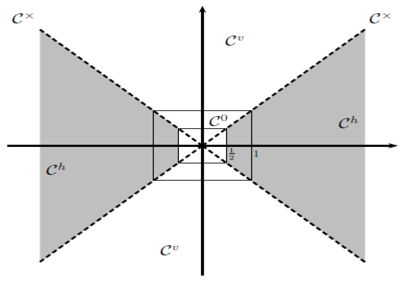
2.1. Continuous Shearlet Transform
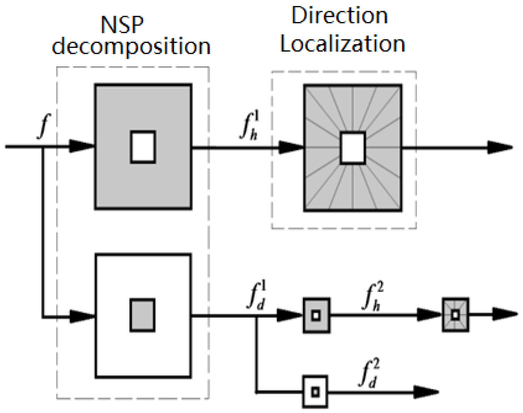
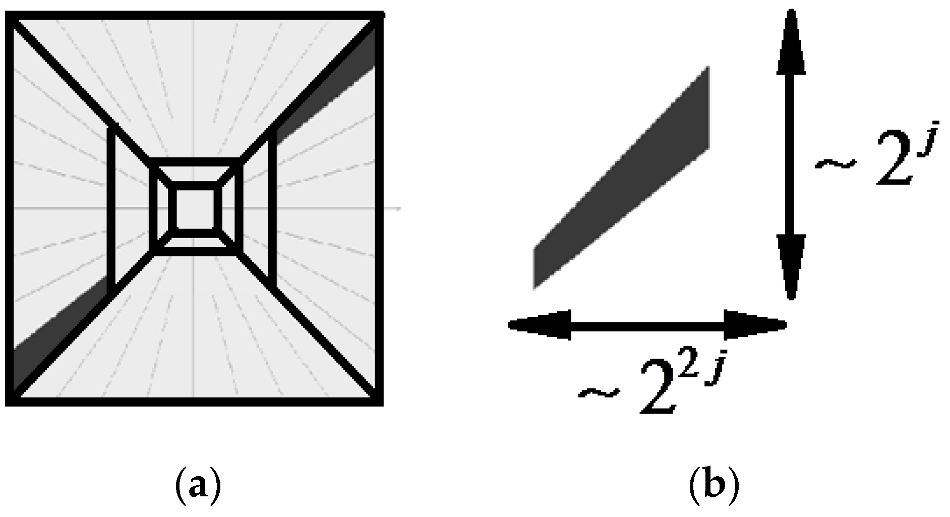
2.2. Discrete Shearlet Transform
3. Separation of Surface Topography Based on FFST
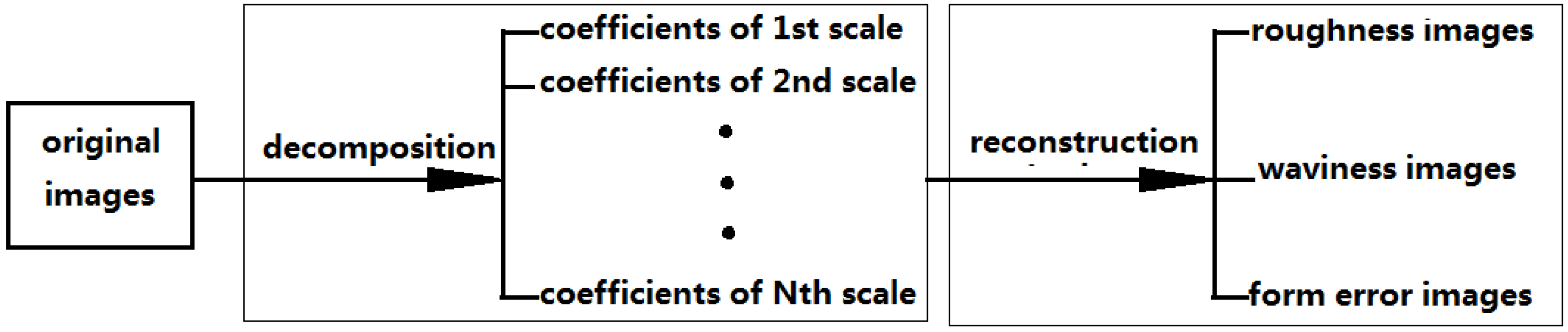
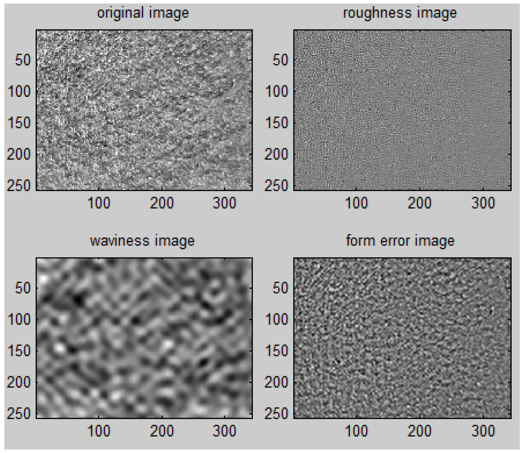
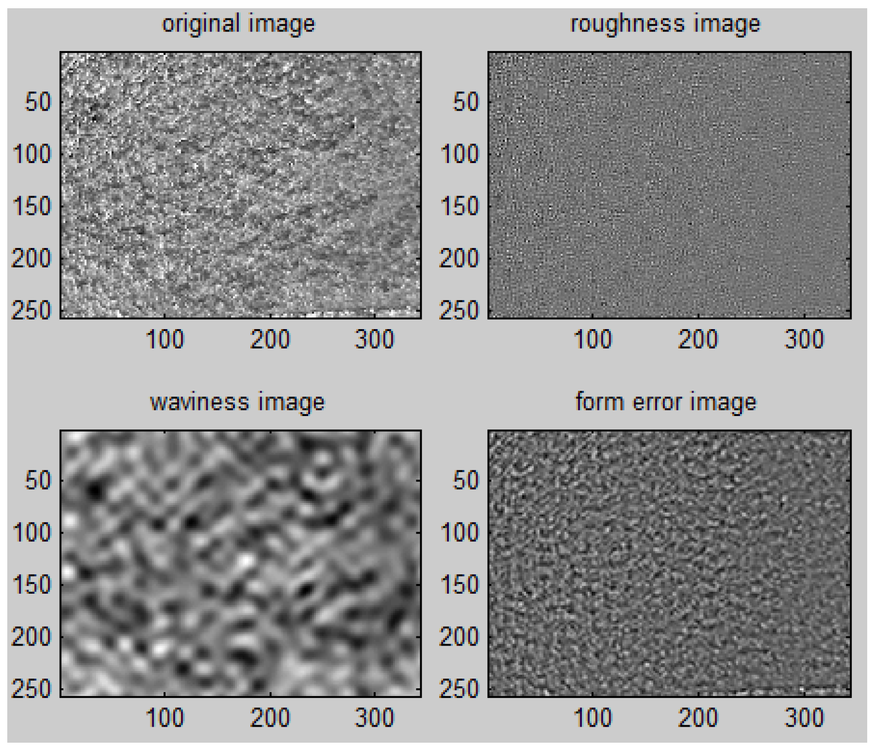
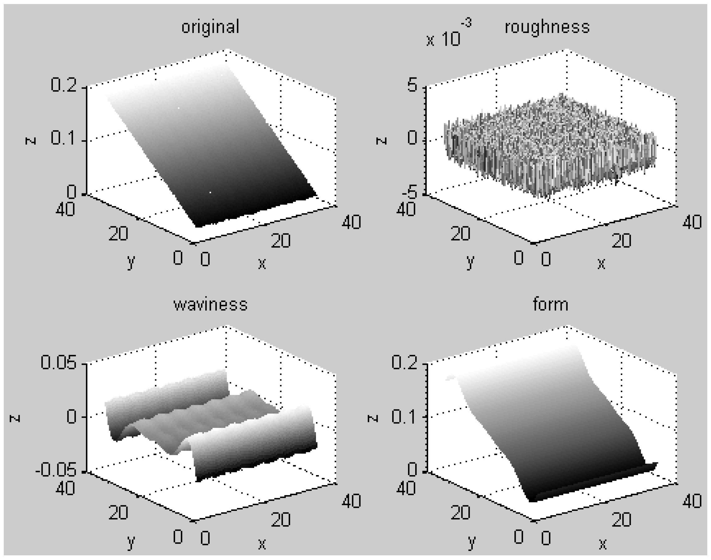
3.1. Decomposition of Surface Topography
3.2. Reconstruction of Surface Topography
3.3. Simulation of Decomposition and Reconstruction for Separating Surface Topography
4. Feature Extraction of Topography Images by a Gray Level Co-Occurrence Matrix
4.1. Principle of the Gray Level Co-Occurrence Matrix
4.2. Feature Extraction of Image Texture
5. Experiment
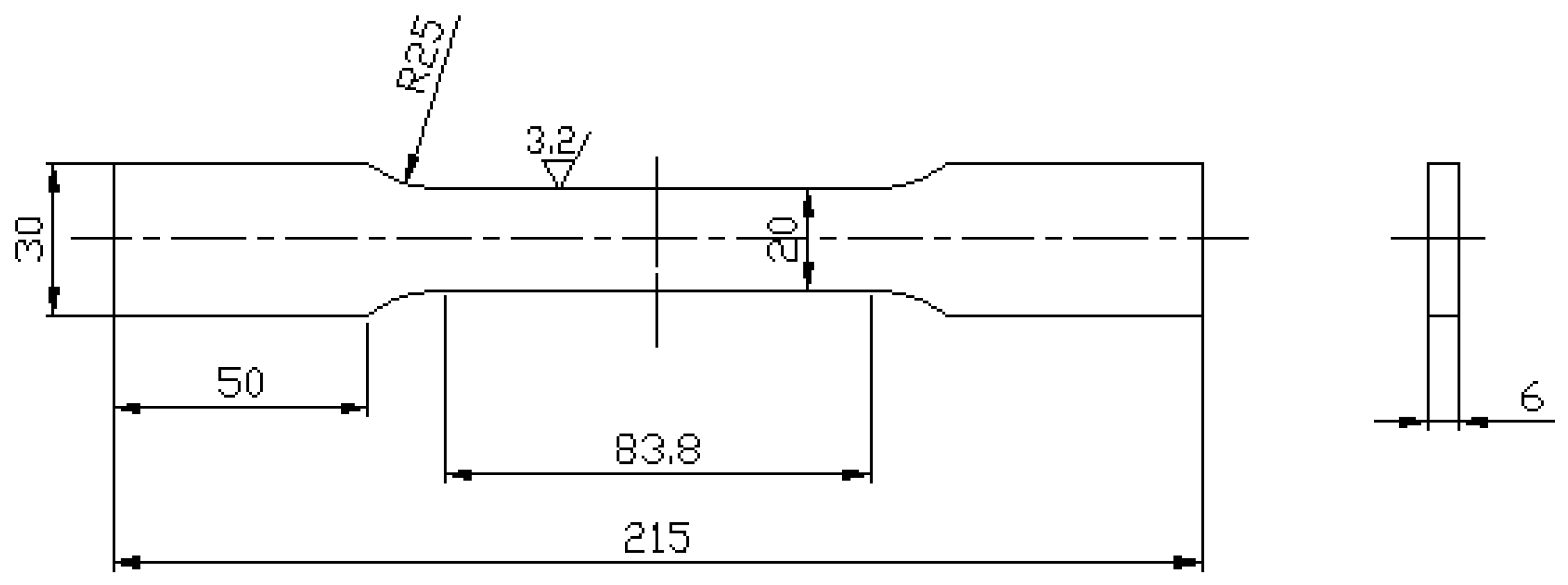
5.1. Description
5.2. Analysis and Discussion
- (1)
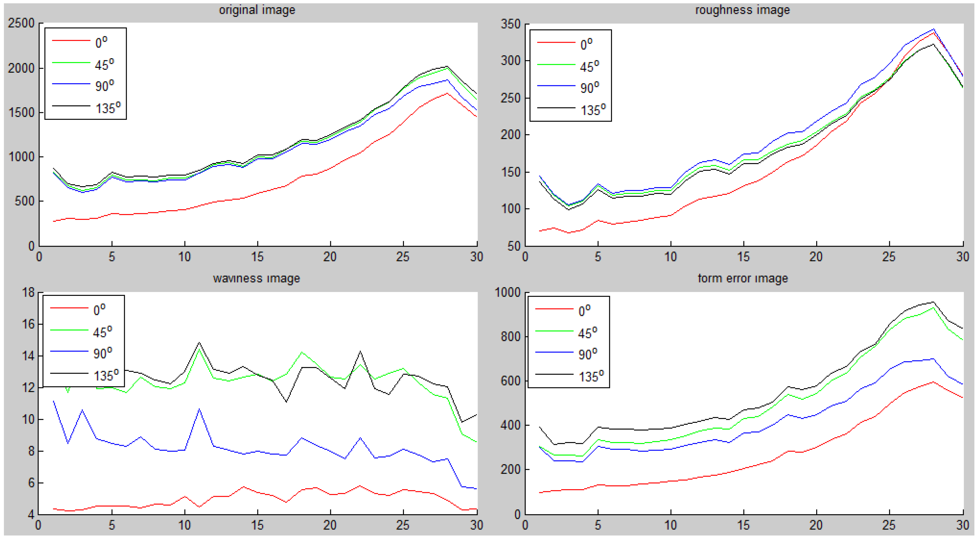
- As fatigue load is applied, the contrast of the surface topography image increases to a maximum, and then decreases before fracture. This occurs mainly because the stress concentration initiates microcracks on the surface and deepens pre-existing crack grooves. As fatigue loading continues, the specimen gradually draws closer to failure, the internal elastic energy releases, and the contrast of the surface topography image decreases.
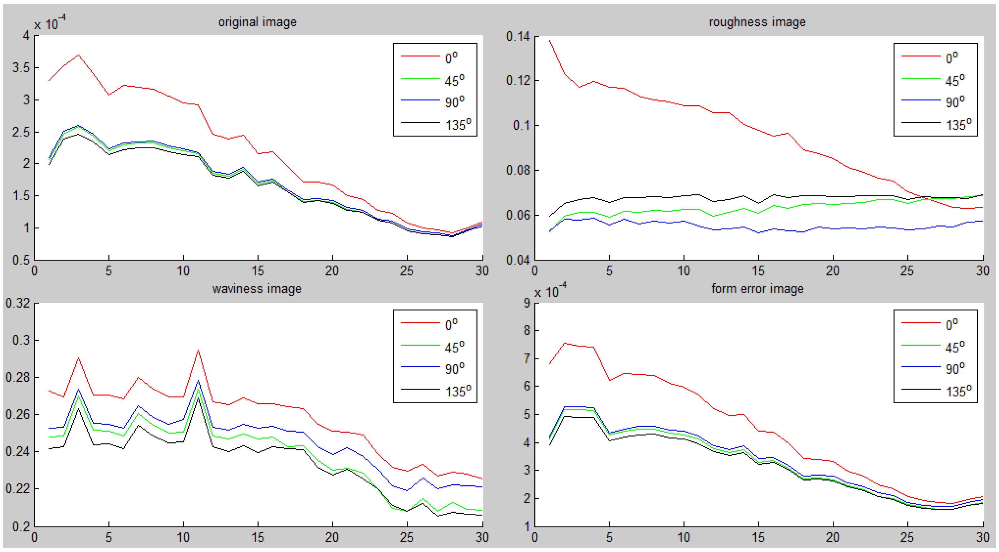
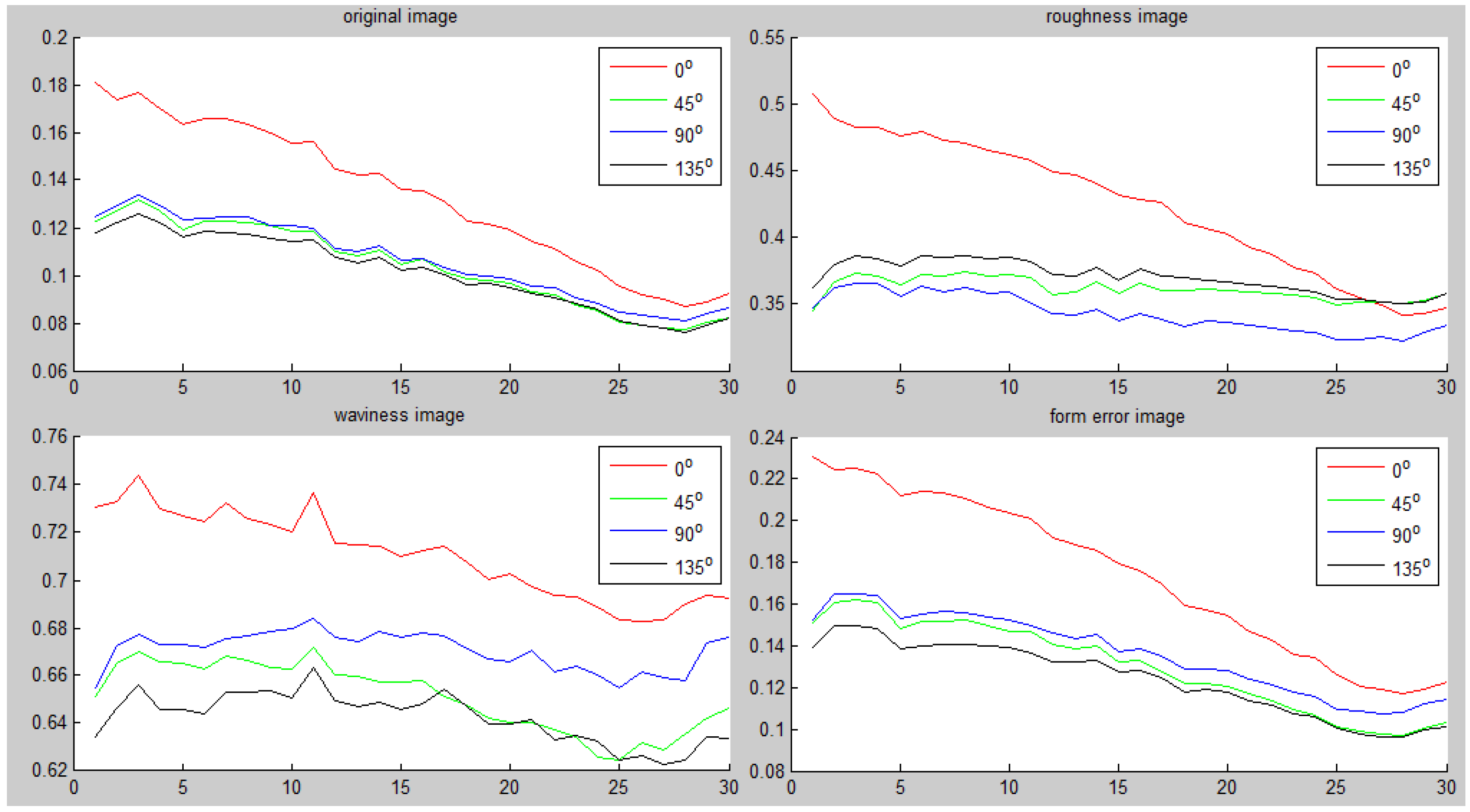
- (2)
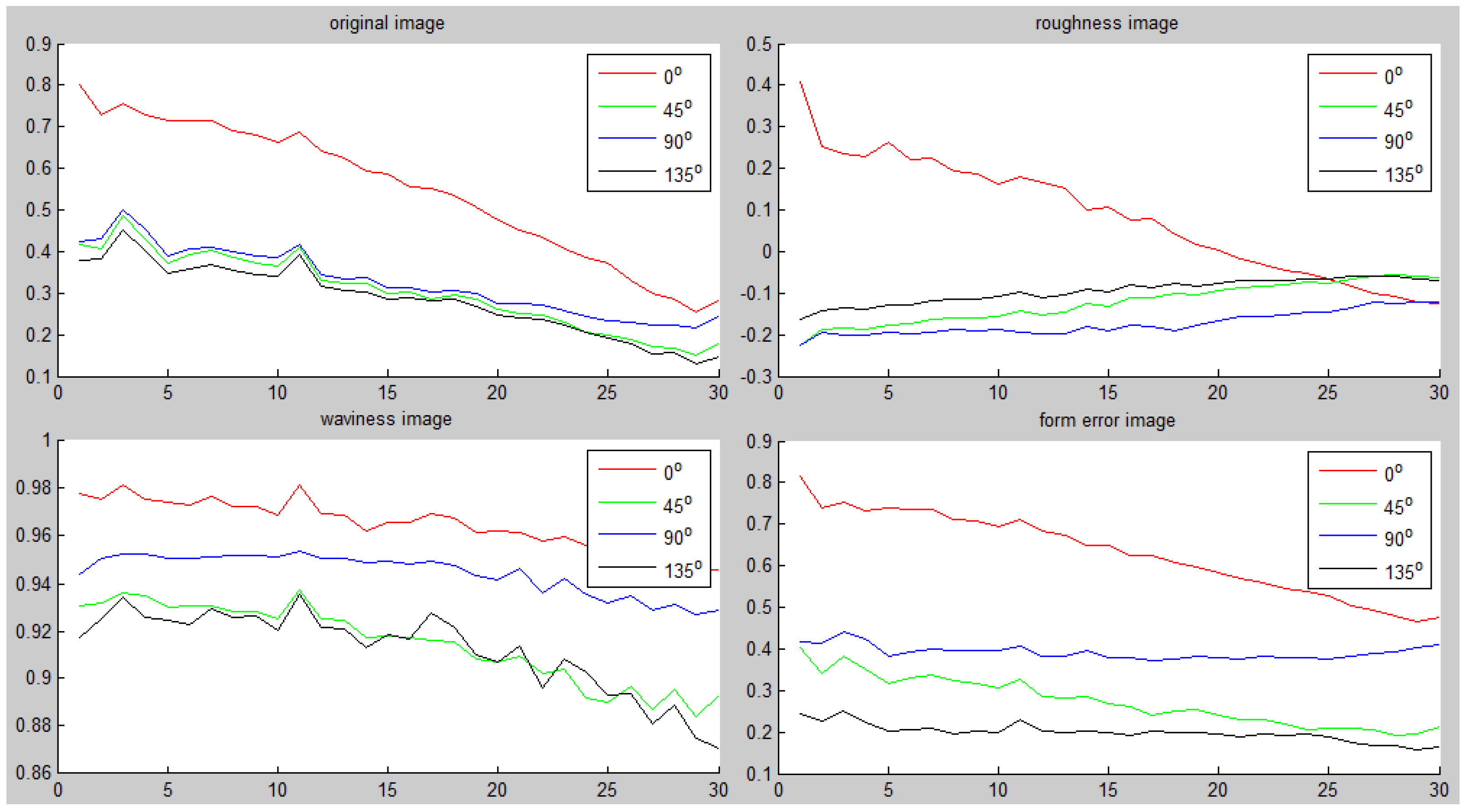
- With fatigue loading, the image correlation coefficient, energy, and entropy decrease and reach their minimums before fracture. The reason perhaps is that the surface grooves deform and the surface texture becomes finer due to “intrusion-extrusion” effects, weakening the texture similarity in all directions and changing it from striped to non-striped.
- (3)
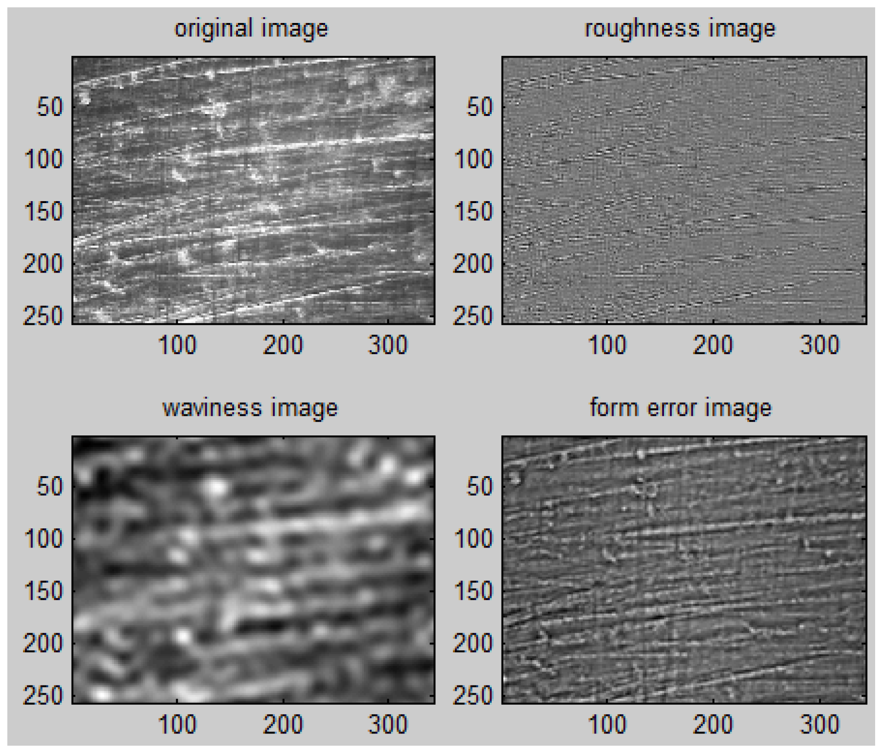
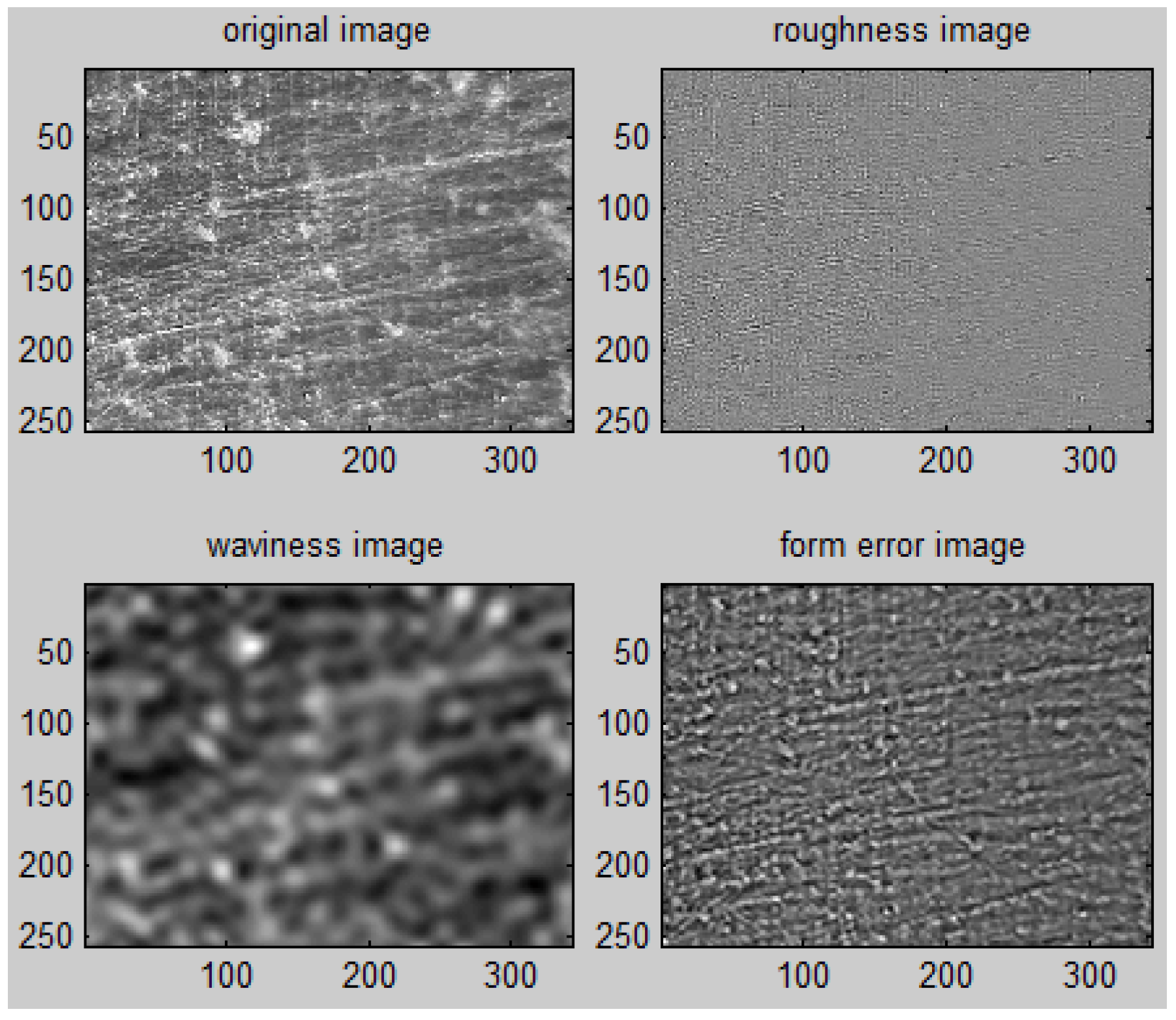
- The decomposition images of roughness obtained by FFST are more similar to the raw images of texture than to the images of waviness and form error. The reason might be that the experimental images are taken of a surface topography in which the surface roughness is more prominent and the fatigue damage manifested firstly as changes in roughness. Moreover, the images of waviness and form error can provide more data useful in recognizing fatigue damage, revealing certain heuristics.
- (4)
- The features of 0° change are more remarkable than those in the other directions. This behavior illustrates that the changes in surface topography with fatigue damage are related to not only the gripping points at the two ends of the specimen, the modes of telescope vertical fixation, and the push-pull impact fatigue testing, but also the direction of fatigue damage.
6. Conclusions
Acknowledgments
Author Contributions
Conflicts of Interest
References
- Whitehouse, D.J. Surface metrology. Meas. Sci. Technol. 1997, 8, 955–972. [Google Scholar] [CrossRef]
- Ardi, D.T.; Li, Y.G.; Chan, K.H.K.; Blunt, L.; Bache, M.R. The effects of machined topography on fatigue life of a nickel based super alloy. Procedia CIRP 2014, 13, 19–24. [Google Scholar] [CrossRef]
- Gao, Y.X.; Yi, J.Z.; Lee, P.D.; Lindley, T.C. A micro-cell model of the effect of microstructure and defects on fatigue resistance in cast aluminum alloys. Acta Mater. 2004, 52, 5435–5449. [Google Scholar] [CrossRef]
- Meng, B.; Guo, W.L.; Jiang, Y. Effect of surface topography on micro-mechanical behavior for different metallic materials. J. Aeronaut. Mater. 2006, 26, 18–23. (In Chinese) [Google Scholar]
- Sachtleber, M.; Raabe, D.; Weiland, H. Surface roughening and color changes of coated aluminum sheets during plastic straining. J. Mater. Process. Technol. 2004, 148, 68–76. [Google Scholar] [CrossRef]
- Wichern, C.M.; Cooman, B.C.D.; Tyne, C.J.V. Surface roughness changes on a hot-dipped galvanized sheet steel during deformation at low strain levels. Acta Mater. 2004, 52, 1211–1222. [Google Scholar] [CrossRef]
- Shigemi, S.; Yasuo, O. Some experimental studies of fatigue slip bands and persistent slip bands during fatigue process of low-carbon steel. Eng. Fract. Mech. 1979, 12, 531–540. [Google Scholar] [CrossRef]
- Ummenhofer, T.; Medgenberg, J. Numerical modelling of thermoelasticity and plasticity in fatigue-loaded low carbon steel. Quant. Infrared Thermogr. J. 2006, 3, 71–91. [Google Scholar] [CrossRef]
- Wang, Y.; Meletis, E.I.; Huang, H. Quantitative study of surface roughness evolution during low-cycle fatigue of 316L stainless steel using Scanning Whitelight Interferometric (SWLI) Microscopy. Int. J. Fatigue 2013, 48, 280–288. [Google Scholar] [CrossRef]
- Liu, C.; Du, S.; Xi, L. Shearlet-based filtering method for three-dimensional engineering surfaces. Mach. Des. Res. 2014, 40, 70–76. (In Chinese) [Google Scholar]
- Wang, M.; Xi, L.; Du, S. 3D surface form error evaluation using high definition metrology. Precis. Eng. 2014, 38, 230–236. [Google Scholar] [CrossRef]
- Suriano, S.; Wang, H.; Hu, S.J. Sequential monitoring of surface spatial variation in automotive machining processes based on high definition metrology. J. Manuf. Syst. 2012, 31, 8–14. [Google Scholar] [CrossRef]
- Yang, G.G. Modern Optical Testing Technology; Zhejiang University Press: Hangzhou, China, 2004. [Google Scholar]
- Tong, X.Y.; Li, H.X.; Yao, L.J.; Li, B. Feature extraction and analysis of surface microscopic image of pure copper subjecting low cycle fatigue. Mech. Sci. Technol. Aerosp. Eng. 2015, 34, 1446–1450. (In Chinese) [Google Scholar]
- Liu, L.; Kuang, G.Y. Overview of image textural feature extraction method. J. Image Graph. 2009, 14, 622–635. (In Chinese) [Google Scholar]
- Guo, K.; Labate, D. Optimally sparse multidimensional representation using shearlets. SIAM J. Math Anal. 2007, 39, 298–318. [Google Scholar] [CrossRef]
- Li, B.; Tang, C.; Zhu, X.; Su, Y.; Xu, W. Shearlet transform for phase extraction in fringe projection profilometry with edges discontinuity. Opt. Lasers Eng. 2016, 78, 91–98. [Google Scholar] [CrossRef]
- Labate, D.; Lim, W.Q.; Kutyniok, G.; Weiss, G. Sparse Multidimensional Representation using Shearlets. SPIE. Digit. Libr. 2005. [Google Scholar] [CrossRef]
- Häuser, S.; Steidl, G. Convex multiclass segmentation with shearlet regularization. Int. J. Comput. Math. 2013, 90, 62–81. [Google Scholar] [CrossRef]
- Haralick, R.M.; Shanmugam, K.; Dinstei, I.H. Textural feature for image classification. IEEE Trans. Syst. Man Cybern. 1975, SMC-3, 610–621. [Google Scholar] [CrossRef]
- Wang, Z.Z. Research on the Classification Method of Remote Sensing Images Based on Texture and Spectral Information Fusion; Xi’an Electronic and Science University: Xi’an, China, 2010. (In Chinese) [Google Scholar]


| Fe | Mn | Cr | Co | P | S |
|---|---|---|---|---|---|
| 93.608% | 0.147% | 0.044% | 0.081% | 0.042% | 0.045% |
© 2017 by the authors. Licensee MDPI, Basel, Switzerland. This article is an open access article distributed under the terms and conditions of the Creative Commons Attribution (CC BY) license ( http://creativecommons.org/licenses/by/4.0/).
Share and Cite
Zhu, D.; Xu, L.; Wang, F.; Liu, T.; Lu, K. Evolution of Metal Surface Topography during Fatigue. Metals 2017, 7, 66. https://doi.org/10.3390/met7020066
Zhu D, Xu L, Wang F, Liu T, Lu K. Evolution of Metal Surface Topography during Fatigue. Metals. 2017; 7(2):66. https://doi.org/10.3390/met7020066
Chicago/Turabian StyleZhu, Darong, Lu Xu, Fangbin Wang, Tao Liu, and Ke Lu. 2017. "Evolution of Metal Surface Topography during Fatigue" Metals 7, no. 2: 66. https://doi.org/10.3390/met7020066