4. Results
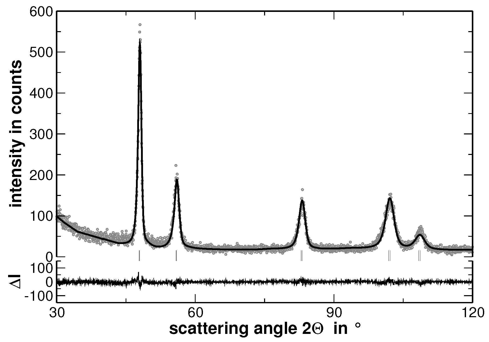
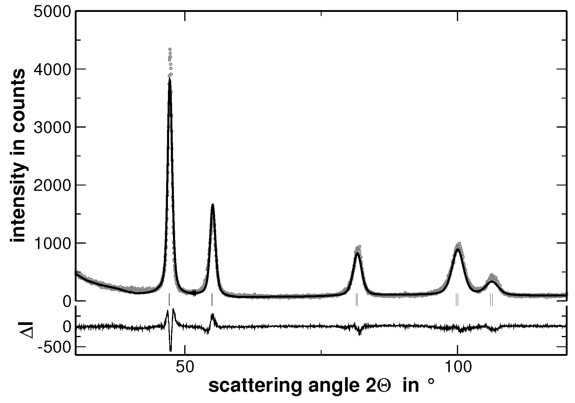
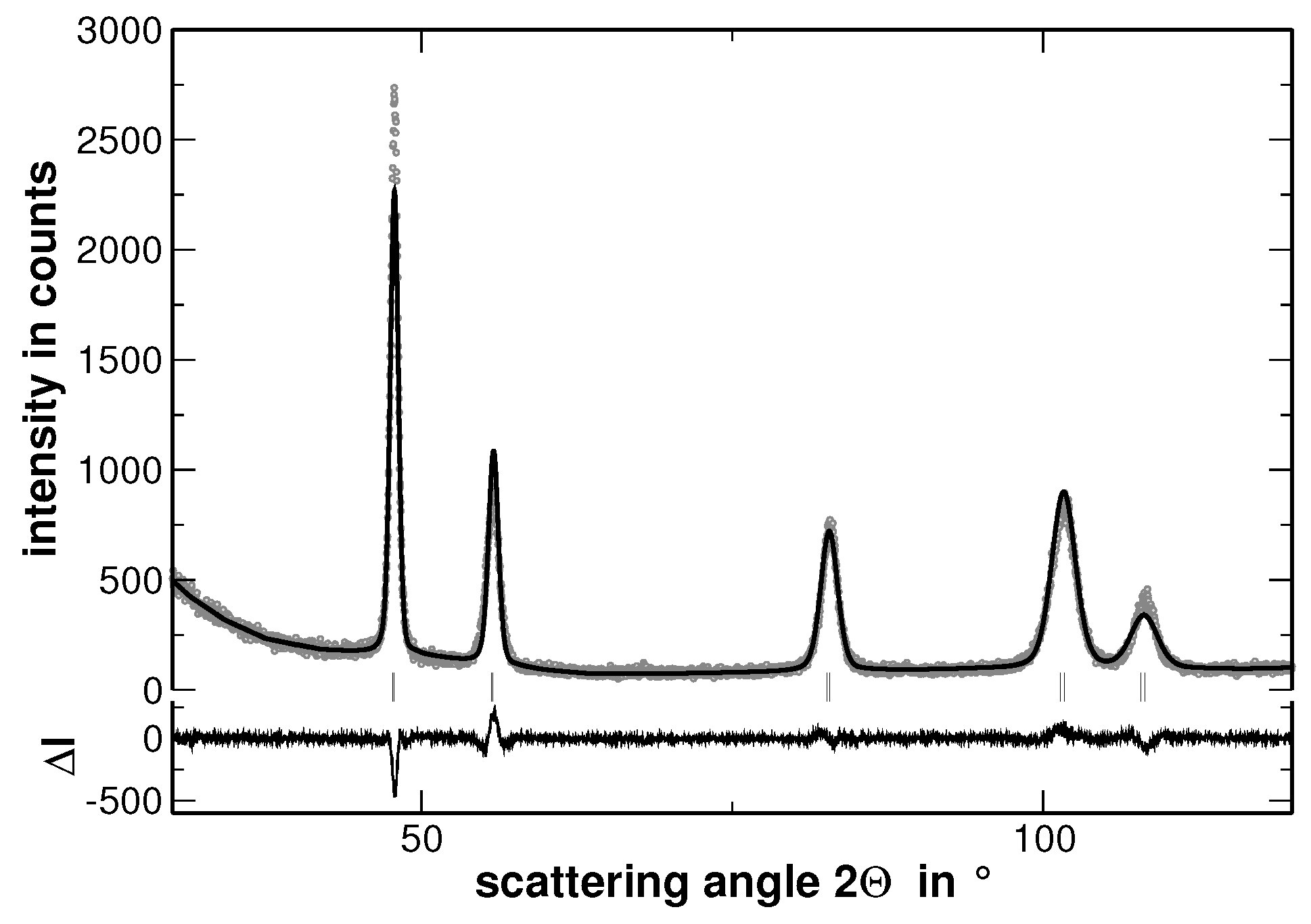
Samples with the composition AuCuNiPd, AuCuNiPt, AuCuPdPt, AuNiPdPt, CuNiPdPt and AuCuNiPdPt were prepared and investigated by XRD. As a typical example, the XRD pattern of AuCuNiPt is presented in
Figure 1.
The XRD experiments reveal that all samples show a face centered cubic (fcc) structure (The XRD patterns, including the corresponding Rietveld analysis, which are not used for discussion are shown in
Appendix A). No traces of secondary phases were detected. Nevertheless, the line broadening is significant even in the homogenized state. This line-broadening, as will be shown in the present article, originates from two major contributions: (i) local lattice strains and (ii) variations of the interplanar spacing, i.e., different lattice parameters, within the sample. The latter originates from segregations. In consequence, and in order to ease the visualization of the effect of segregations on line-broadening, the sample was further heat treated to widen the elemental distribution of the segregation. Before the effect of segregations is displayed, the homogenized state is characterized in the following.
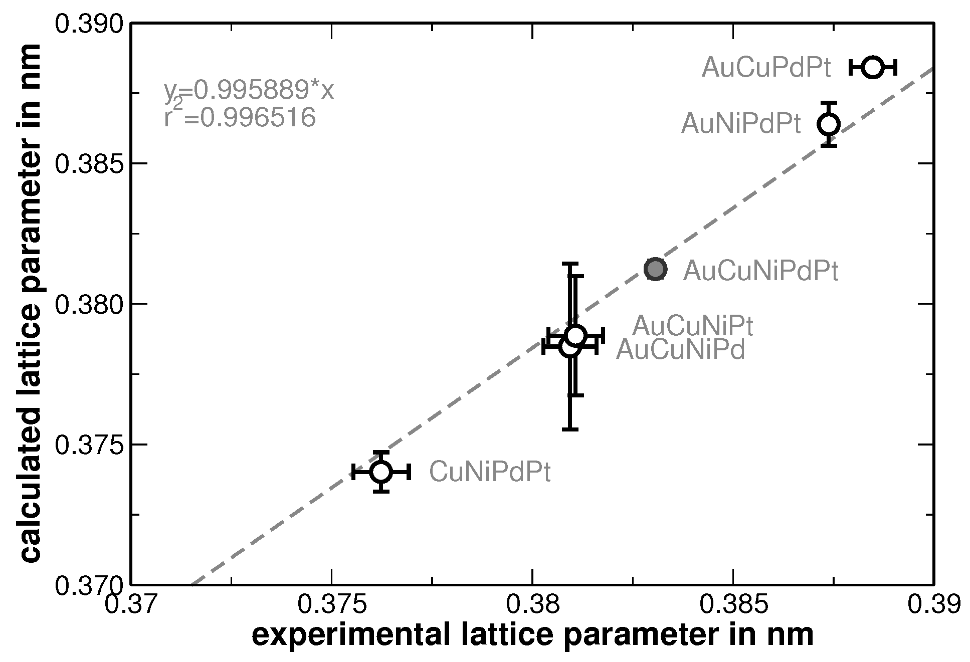
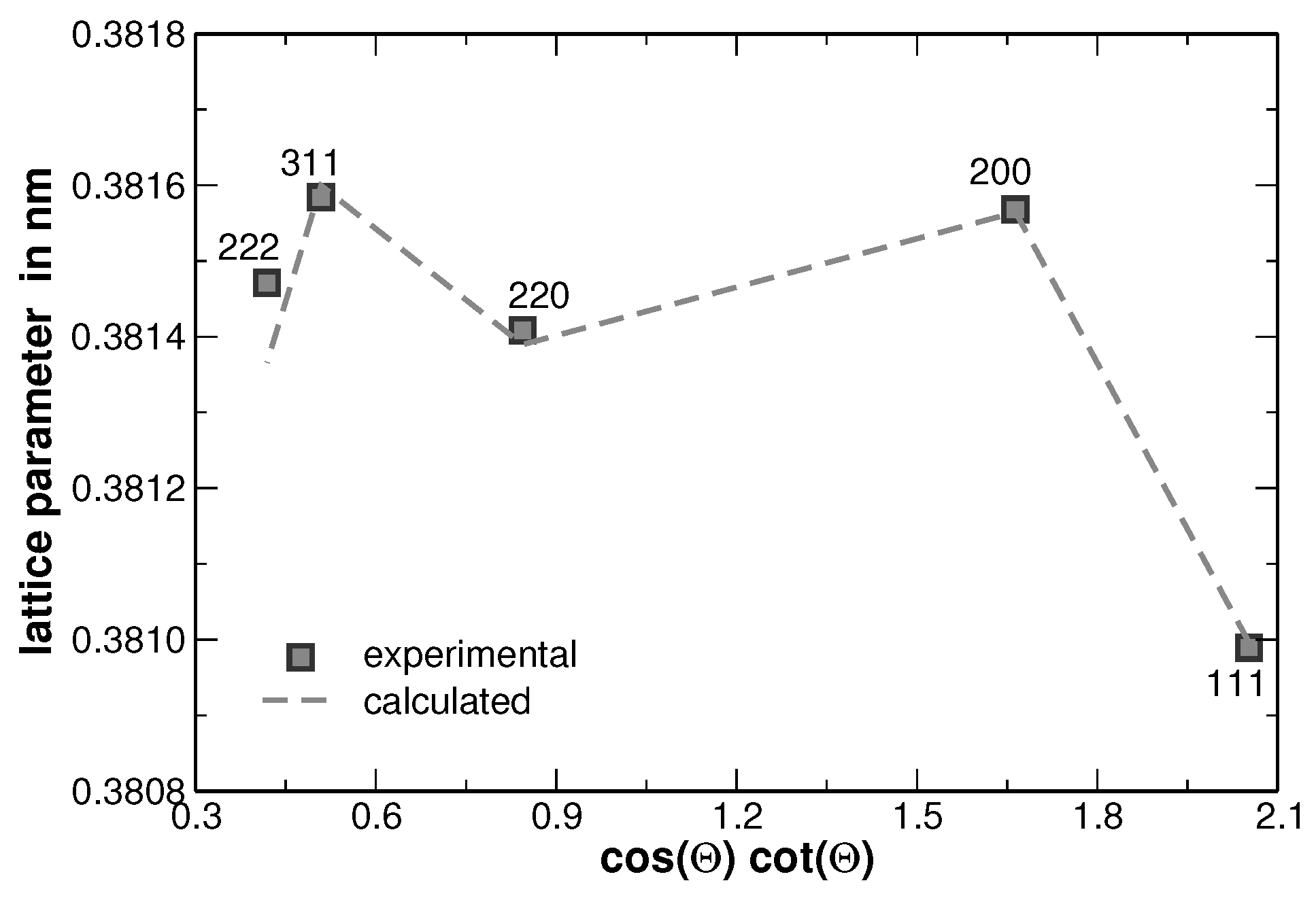
The increase of the background at low scattering angles originates from the silicone grease used to fix the samples and should not be of further interest. The Rietveld analysis revealed that the average lattice parameter of the alloy follows the Vegard’s rule of mixture. In order to stress the validation of this rule, the experimentally determined lattice parameter of the samples has been compared to that ones calculated upon the actual sample composition, as shown in
Figure 2.
Table 1 summarizes the values used. The mean sample composition and its spatial fluctuations were determined by EDX measurements as described in the following.
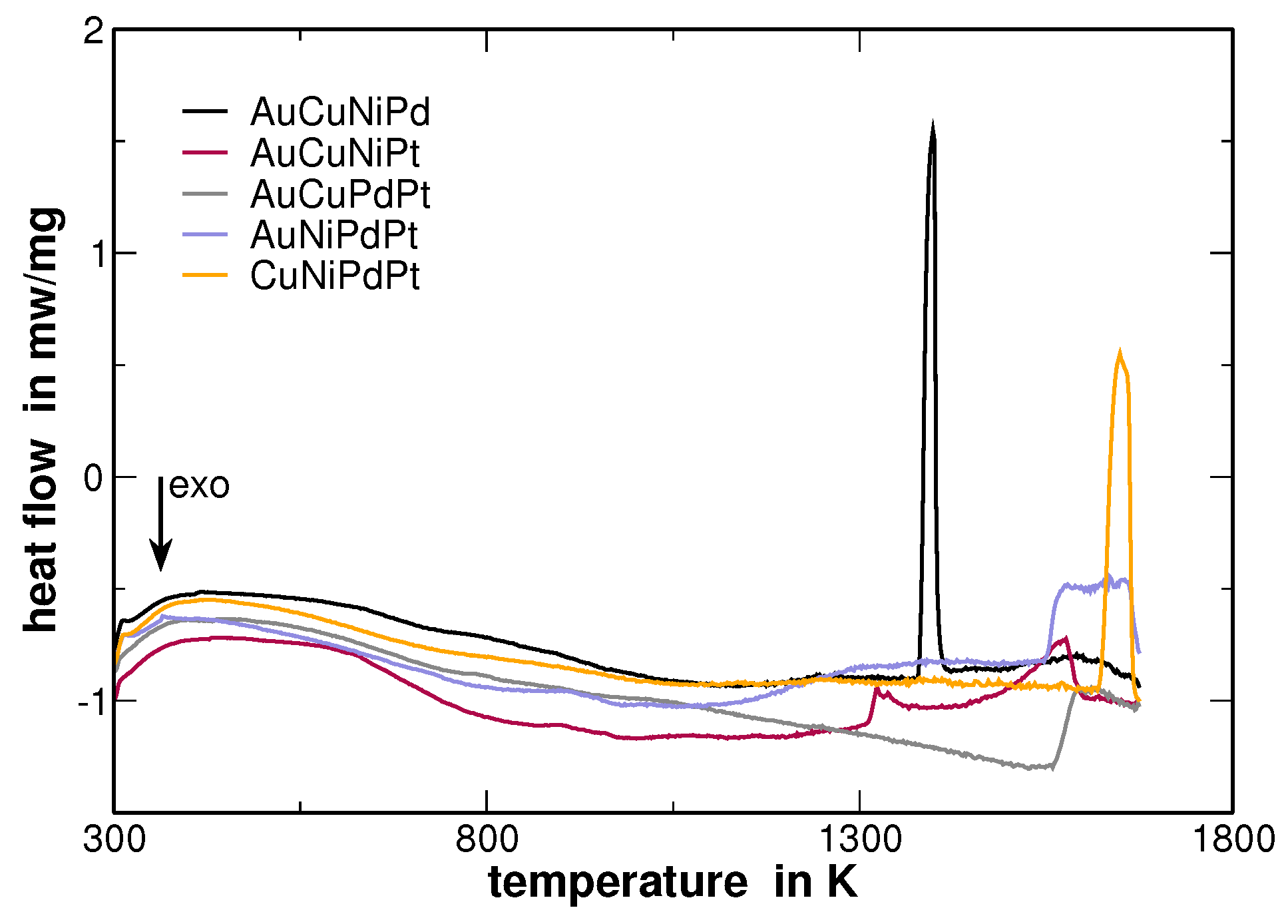
The errors depicted for the experimentally determined lattice parameters were taken from the Rietveld analysis, while the errors of the calculated lattice parameters originate from the locally observed variations of the composition as described in the following. The latter errors reflect segregations that have been obtained from a second heat treatment after homogenization. Large segregation was observed for AuCuNiPt. DSC measurements show the onset of melting at
and a melting range up to
(the DSC curves are provided in
Appendix B). The second heat treatment was performed in the two-phase region above the solidus and below the liquidus temperature in order to promote the formation of segregations. Hence, this sample was heat treated at
for
and subsequently water-quenched. It turned out that this heat treatment did not alter the spread of the elemental distribution, when compared to the as-cast state. Furthermore, the XRD patterns essentially appeared similar, which is obvious when considering that the measurements were performed on crushed powders. However, the microstructure was coarsened. Heat treatments at lower temperatures, ranging from
to
were additionally applied. However, these samples do not show this large distribution of concentrations. As expected from DSC measurements, these heat treatments did not result in the formation of secondary phases. When no error bar is shown in
Figure 2, the error is smaller than the symbol size. No second heat treatment was applied to the AuCuNiPdPt alloy, therefore, no significant segregations are determined.
An origin for the highly segregated microstructure observed in AuCuNiPd and AuCuNiPt might be connected to sluggish diffusion [
20]. According to
Table 1 gold atoms have the largest radius among the elements under investigation, while copper and nickel have the smallest radii. The quaternary alloys composed of these three elements (and any fourth one) are expected to show a reduced diffusion rate when compared to alloys composed of atoms with a closer distribution of the metallic radii. In this case, the sluggish diffusion is insufficient to homogenize the highly segregated state. In consequence, the microstructure is comparable to the as-cast state. A wide two-phase (solid + liquid) region might be expected when the melting temperatures of the elements show a large distribution. This could possibly cause large segregations. However, when considering the melting temperatures shown in
Table 1, this is not the case.
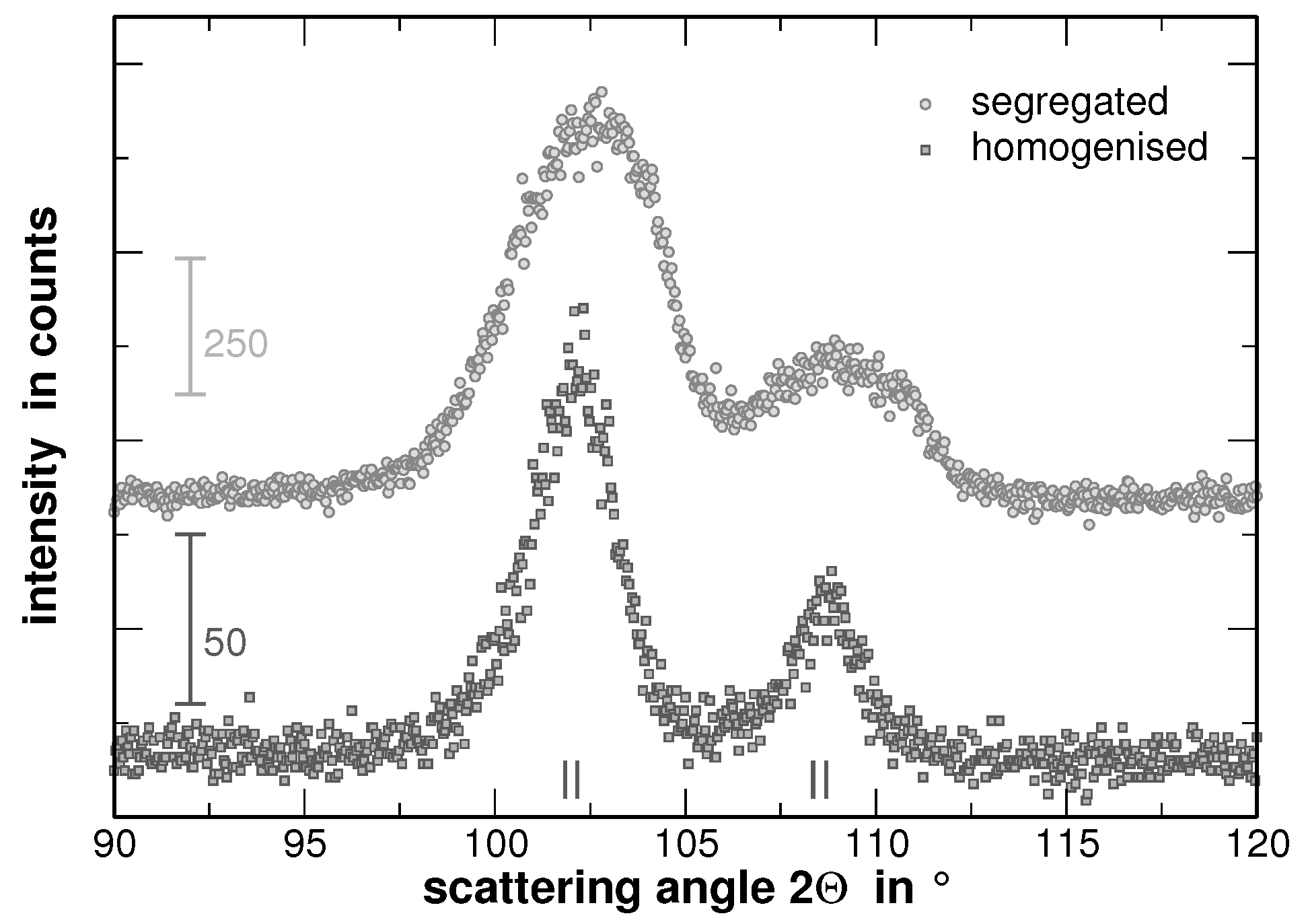
In order to visualize the effect of the second heat treatment, the high-angle range of the XRD patterns taken on the homogenized as well as on the segregated state of AuCuNiPt is shown in
Figure 3. These patterns are cuts from the XRD patterns shown in
Figure 1 and
Figure 4, respectively. The second heat treatment region affects the XRD line profiles as exemplarily shown in
Figure 3 for the 311 and 222 reflections of AuCuNiPt. The shape of the reflections of homogenized samples is of Cauchy type, which turns into a “super Gaussian” type for the segregated sample. The “super Gaussian” line broadening in the segregated state can be interpreted as a convolution of the diffraction lines produced by the homogenized sample with a function describing the distribution of interplanar spacings or local concentrations of individual elements [
21].
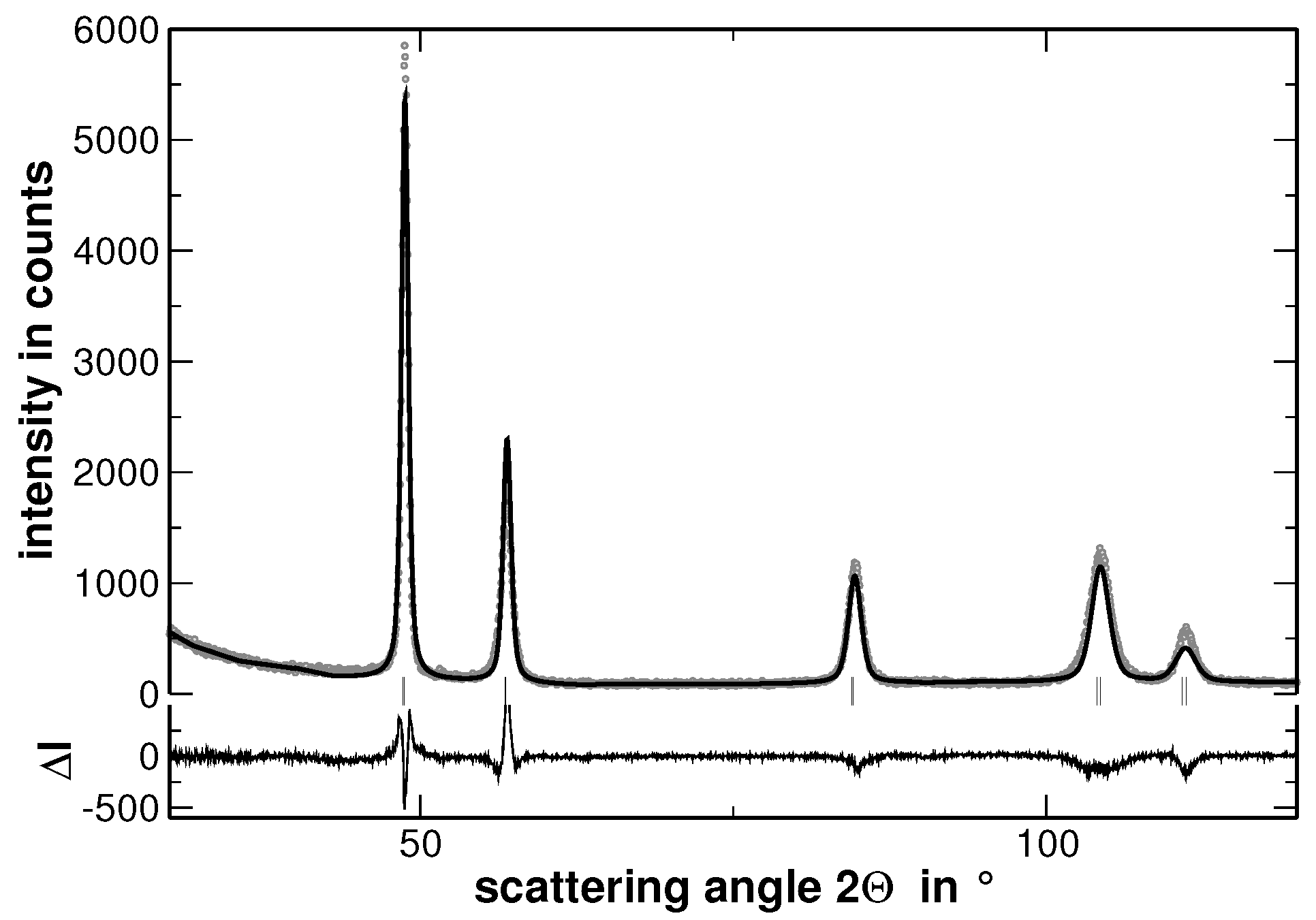
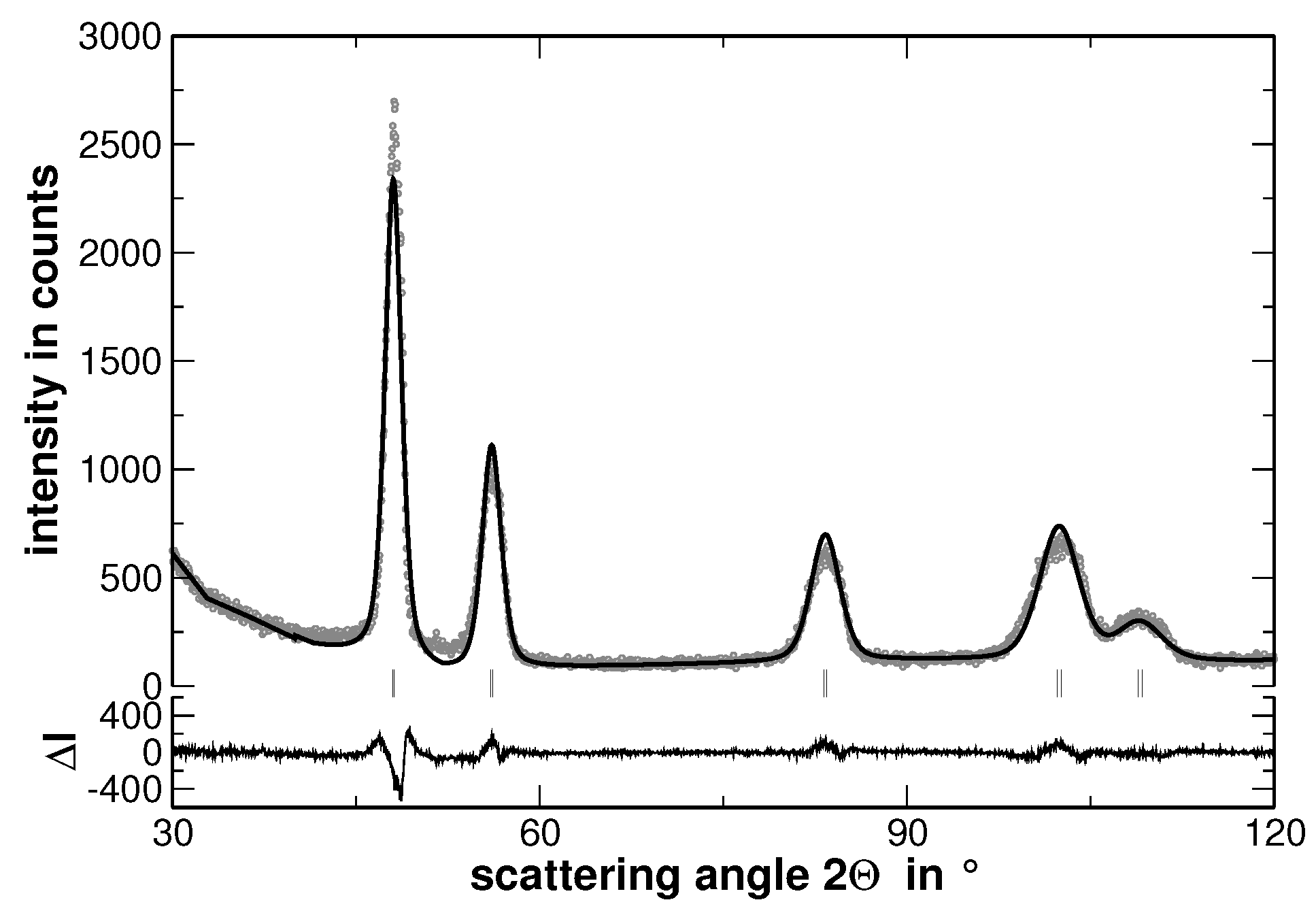
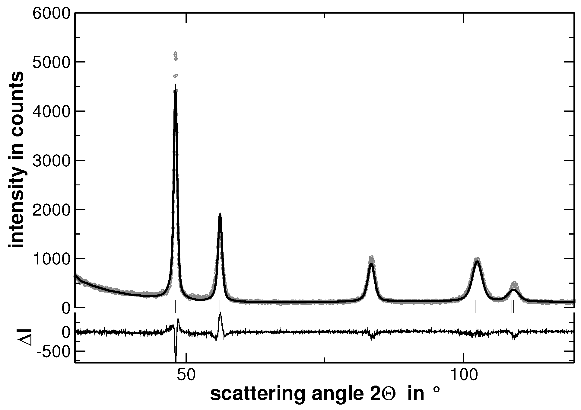
Multi-component solid solutions with significantly different metallic radii of the constituting elements are expected to cause lattice strains that are reflected by an intense diffuse scattering. In contrast, segregations cause a significant contribution to the width of the reflections determined from XRD experiments, especially if they lead to variations of the interplanar spacing. The latter behavior is demonstrated in
Figure 4, where the measured XRD pattern and the corresponding calculated pattern derived by the Rietveld analysis are shown.
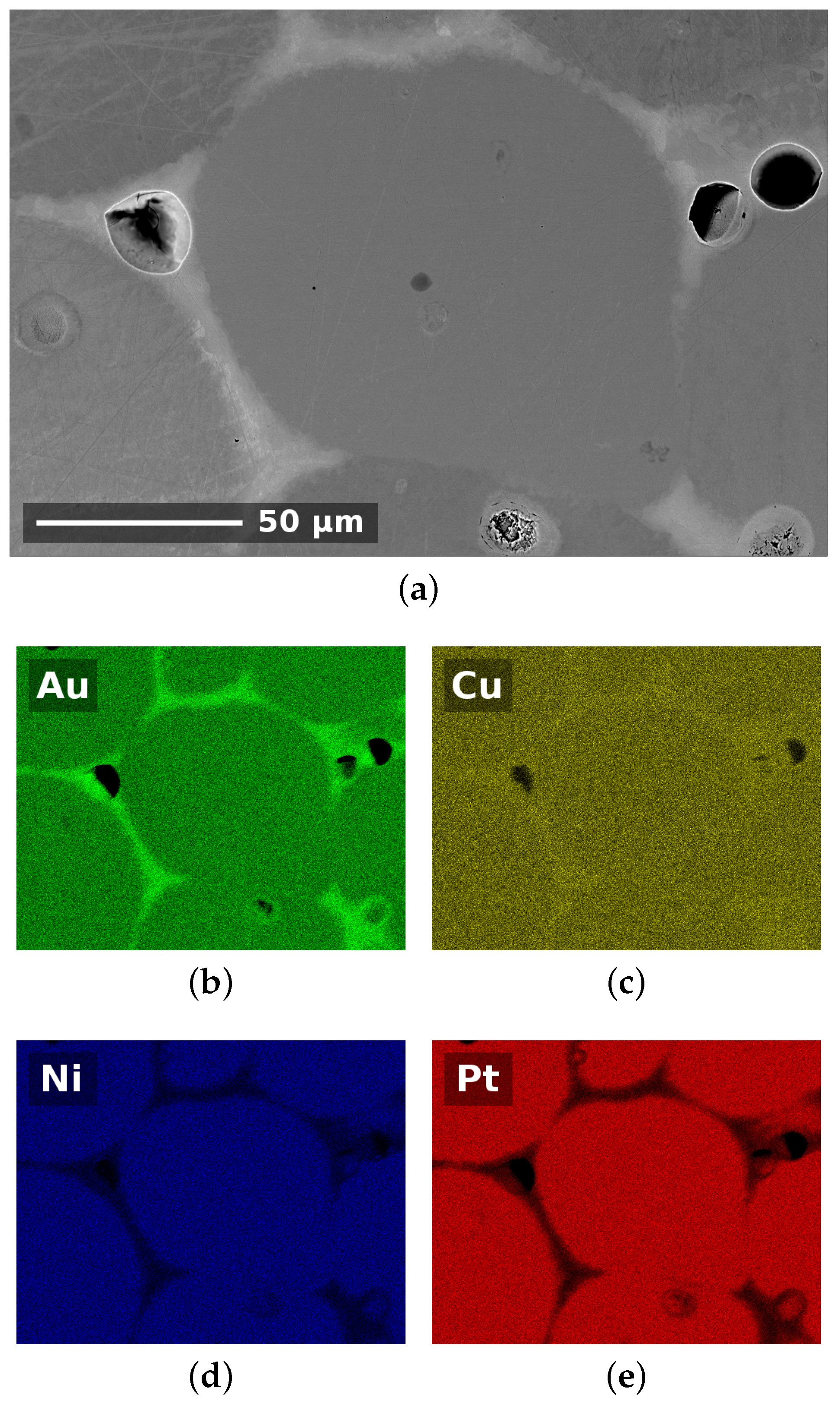
Figure 5 shows the microstructure of the AuCuNiPt alloy in a maximum segregated state as well as elemental mapping images obtained from EDX analysis. The SEM micrograph clearly shows a bright area at the grain boundaries and voids, which arise from the annealing in the two-phase region. This sample is heterogeneous, as it was already indicated by the XRD line broadening. However, it contains only a single fcc phase. The elemental mapping images reveal that the copper and gold atoms segregate to the grain boundaries (
Figure 5b), which were in the liquid state during annealing at
. Furthermore, with respect to the observed distribution of the elements, the grains appear round in shape, which also is interpreted as a consequence of the heat treatment. According to
Table 1 Au and Cu have a comparably low melting temperature when compared to the other alloying elements, which is regarded as an origin of the observed behavior. Besides that, the pair mixing enthalpies of binary alloys influence the preferential pairing of particular elements. According to the enthalpies of mixing (as provided in
Appendix C) Au-Ni, Cu-Ni and Au-Pt binary bonds are non-preferential in a 1:1 mixture of the elements, while Au-Cu, Ni-Pt and Cu-Pt should be preferred. With the exception of the binary Cu-Pt bonds, this behavior is also reflected by the observed segregation. The grain boundary is enriched in Au and Cu, i.e., presumably showing a larger number of Au-Cu bonds, and the grain interior is enriched in Ni and Pt, which can be linked to the preference of forming binary Ni-Pt bonds. In addition, Pt has a higher melting temperature than Cu. In consequence, the melt would be rich in Cu and poor in Pt, which is also reflected by the observed elemental distribution shown in
Figure 5. Due to this fact, the preference for the Cu-Pt bond cannot be realized and, furthermore, hinders a stronger Cu segregation to the grain boundary in comparison to Au (this is also reflected by
Table 2). With the same reasoning, the huge differences in melting intervals between the different alloys as shown in
Figure A6 (
Appendix B) becomes understandable.
The elemental mappings were not corrected with respect to the atomic number, absorption or fluorescence (ZAF correction). Hence, they are believed to provide qualitative information, only. Nevertheless, this information is further used to evaluate the local elemental distribution of the sample.
The EDX maps were collected with a resolution of
pixels of which 98.6% were actually considered to provide suitable composition data. The residual pixels are attributed to the voids apparent in
Figure 5. The EDX mappings were re-evaluated according to the following scheme. Utilizing the Mathematica software, the four EDX maps had been transferred into a spreadsheet containing the pixels as well as the colors, which were further processed to the elemental concentration, while zero color saturation equals to zero concentration and maximum color saturation equals to full concentration. For each elemental map, the average value of all pixels under investigation was adjusted to the value obtained from a ZAF corrected areal EDX analysis. The area of this analysis was identical to that of the elemental mappings. The result of this EDX analysis is shown in
Table 2. In order to confirm that this local elemental analysis matches the global composition and to demonstrate that it is representative for the whole sample, ICP-OES measurements have been performed. The results are also shown in
Table 2. The results proof that the sample preparation does not cause significant (evaporation) losses.
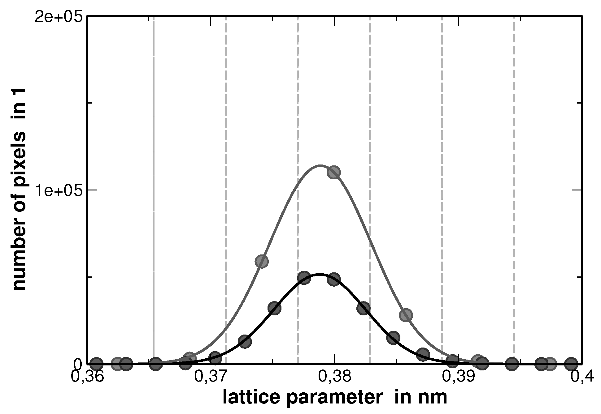
Due to the fact that no correction corresponding adsorption and fluorescence has been applied, the procedure of analyzing the elemental mapping images causes a maximum error of 81%, as the sum of the individual concentrations for each pixel does not sum up to 100%. In order to further evaluate the image, the concentration at each pixel was adapted in a way that the sum of the concentrations at each pixel was normalized to 100%. According to Vegard’s rule of mixture, a lattice parameter was assigned to each pixel. The distribution of the lattice parameters obtained from this analysis is of Gaussian type, as shown in
Figure 6.
The center of this distribution matches the experimental lattice parameter. Although there is a large error within the compositions as determined by EDX for the pixels, the error is compensated by the large statistics.
The distribution functions from
Figure 6 were employed to fit the experimental XRD profiles by a discrete convolution of Gaussian functions. According to Ref. [
22], the discrete convolution can be calculated using:
In Equation (
2),
describes the distribution of the lattice parameters normalized to a unity area and
represents the set of mutually shifted Gaussian functions (in a matrix form). Individual functions
have their maxima at the Bragg angles that correspond to the respective lattice parameters.
are the resulting convoluted intensities. To fit the convoluted intensities to the measured ones, the least-squares algorithm was applied. The only refinable parameter was the width of the Gaussian functions.
In order to take the differences in the scattering power of individual atoms into account, the distribution function
was multiplied by a composition-dependent atomic scattering factor, which was obtained from:
In Equation (
3)
q represents the scattering vector. The coefficients
,
and
c, which are required to determine the atomic scattering factor are provided in
Table A3 in
Appendix D. The factors
are the molar ratios of individual atomic species. As the convolution from Equation (
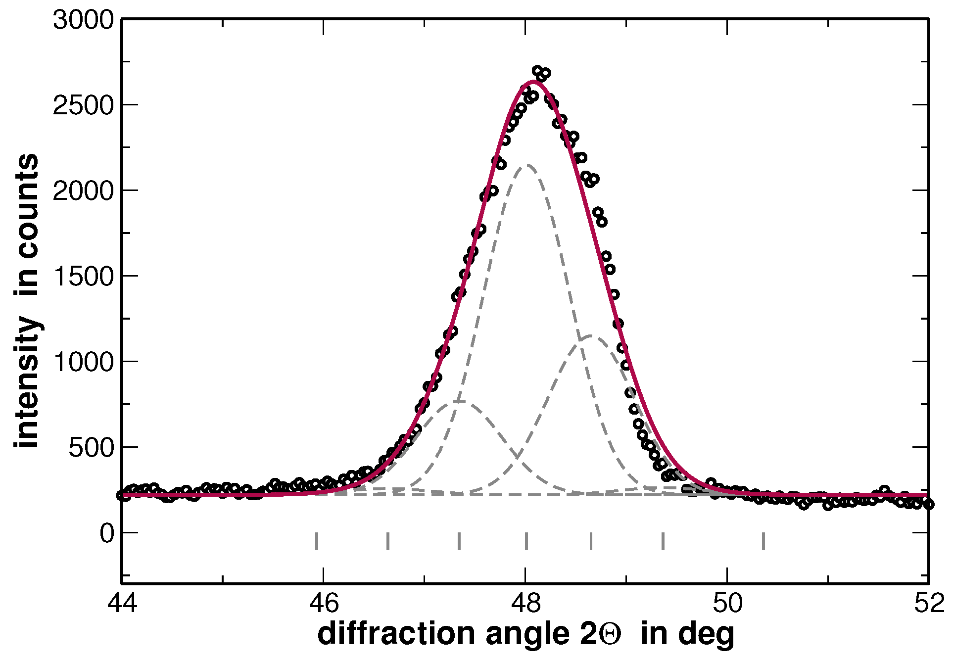
2) relates to the diffraction angles (and thus to the lattice parameters) but not to the local concentrations, the average concentration of the elements within each fraction classed according to the lattice parameter has been used to calculate the atomic scattering factor for simplicity. An example of the diffraction line 111 fitted by using the above procedure is shown in
Figure 7.
The results of the fitting procedure are shown in
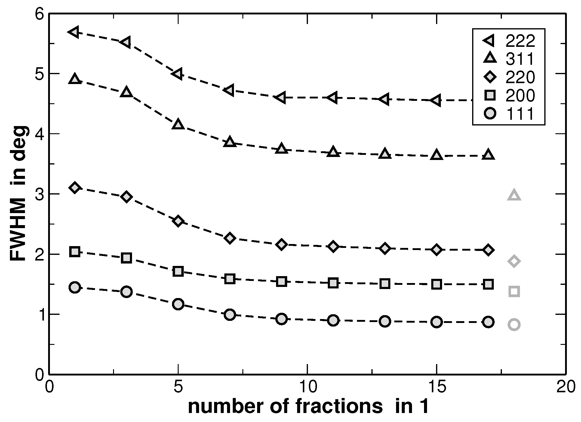
Figure 8. There, the full-width at half-maximum (FWHM) values of the underlying Gaussian profiles are shown for individual diffraction lines and as a function of the fractions used for the line fitting as illustrated in
Figure 7. In principle this is the only fitting parameter of interest, since the ratio of the areas of the underlying Gaussian profiles is kept constant (as it is given by the distribution function from
Figure 6) and the sum is exclusively fitted.
Figure 8 reveals that the FWHM of the underlying Gaussian profiles decreases with increasing number of fractions and saturates at a nearly constant level if more than 10 fractions are used. It is noteworthy that the FWHM of the main reflections saturate at a value 10%–15% higher than the FWHM value obtained for a sample in the homogenized state (the corresponding values are additionally shown in
Figure 8 with grey symbols. The original XRD pattern is presented in
Figure 1). The same procedure was applied to the XRD lines of the homogenized state. However, the results do not reveal a significant variation of the FWHM values with increasing number of fractions. This result is explained by the smaller variation of segregations of regions with different lattice parameters in the homogenized state. Furthermore,
Figure 8 reveals that the line widths obtained from the fitting are strongly anisotropic, i.e., they depend on the crystallographic direction. Still, this anisotropy of the XRD line broadening could be reproduced by the dependence of FWHM on the cubic invariant
as described, e.g., by T. Ungár in [
23,
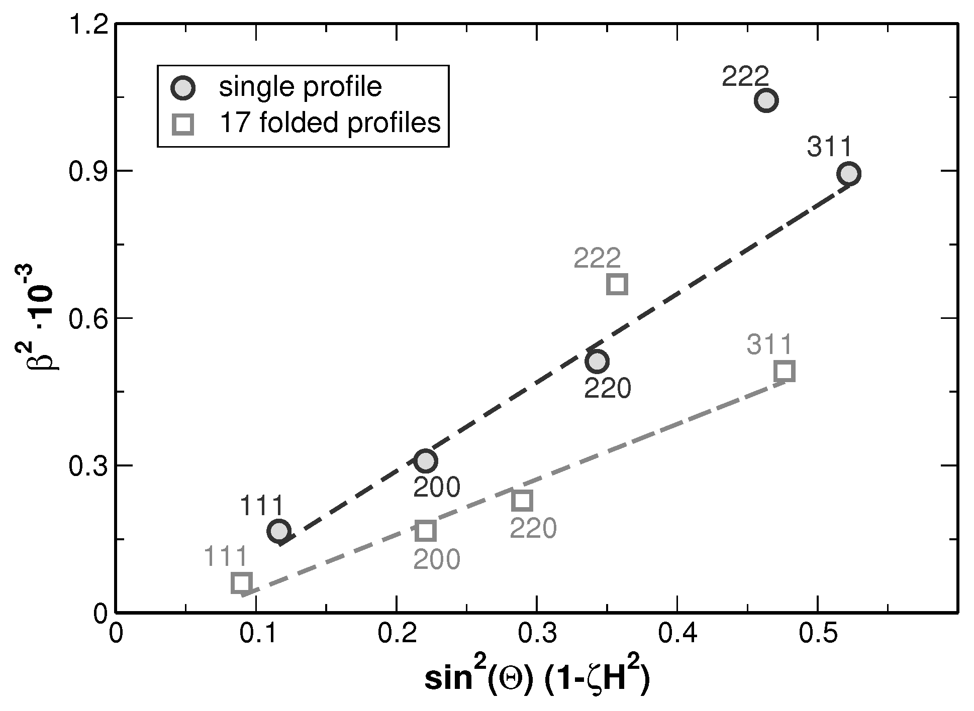
24]. The values obtained for single profile fitting as well as for fitting with 17 folded profiles were used to perform a modified Williamson-Hall analysis [
23,
24,
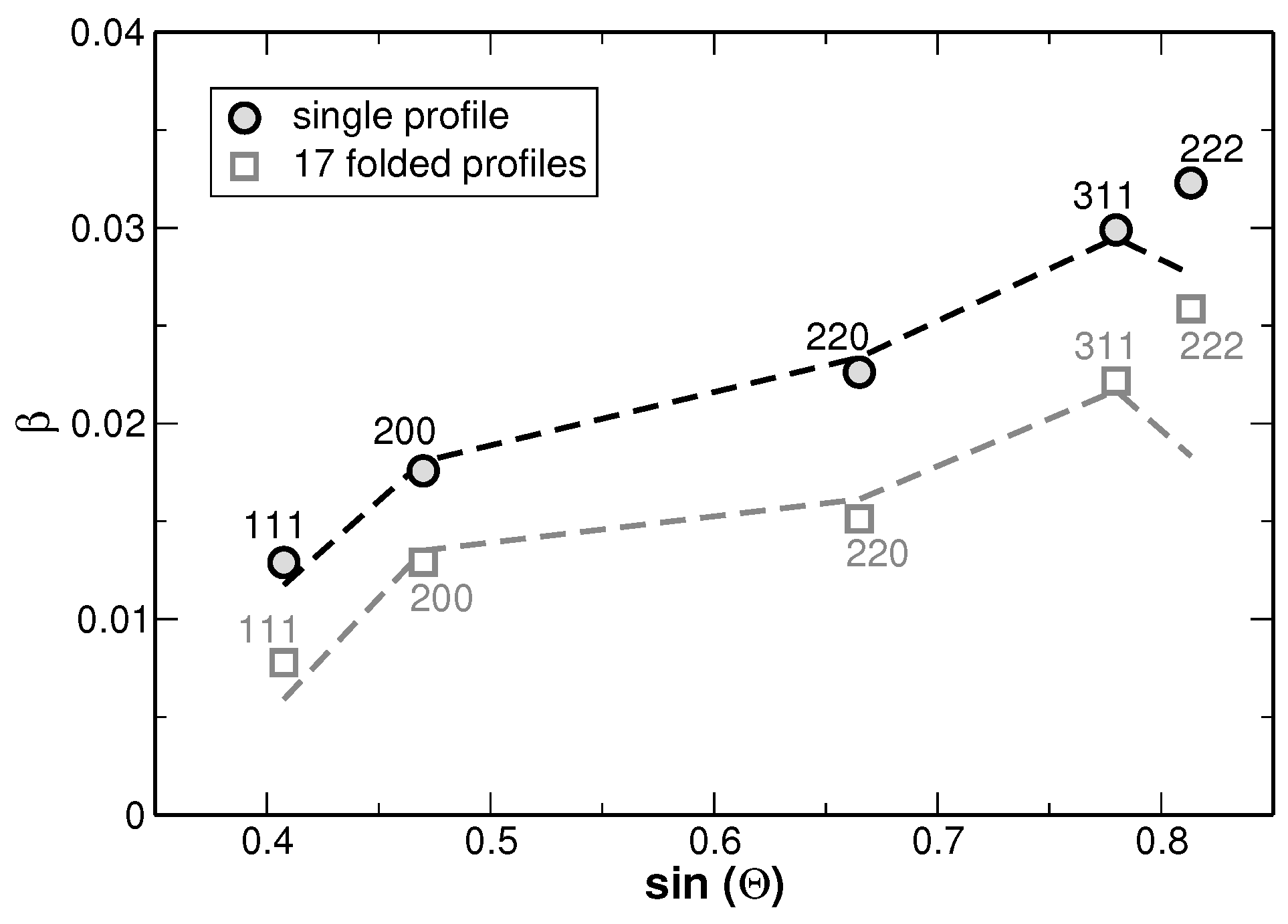
25]. The results are shown in
Figure 9.
As it can be seen from the modified Williamson-Hall plot, a fitting of the values yields a high goodness of fit as far as the 222 reflections are not considered within the evaluation. This appears reasonable since the intensities of these reflections are rather low and the 222 reflections show an overlap with the larger neighboring 311 reflections as can be seen from
Figure 3. Such anisotropy of the line broadening is typically produced by the anisotropy of elastic constants, when local strain fields are present in the crystalline material. The strain fields can originate either from dislocations or from lattice misfit at the crystallite or grain boundaries. These two effects can be distinguished by employing the effect of the strain on the lattice parameter as shown in [
26,
27]. The pronounced dependence of the lattice parameters on the crystallographic direction, as shown in
Figure 10 indicates that the local lattice strain is produced not only by dislocations but also by a kind of the internal boundaries. Without defects influencing the lattice parameters in specific crystallographic directions,
Figure 10 should show a straight extrapolation towards the intercept at
and with a slope which is solely depending on the errors of the measurement. Both modified Williamson-Hall plots from
Figure 9 revealed that the coherently scattering regions are very large, as it can be expected for the grain sizes in the order of
(see
Figure 5). Additionally, the Williamson-Hall analysis provides values for the lattice strain. The strain values determined from these analyses show (i) large values when compared to homogenized single-element metals and (ii) an apparent enhancement which is attributed to segregations. These were separated to access the true lattice strain. This becomes possible since segregations shift the average lattice parameter, which due to the overlay of different composition appears as line-broadening, while lattice distortions cause an intrinsic line-broadening.
Microscopic lattice strains are commonly defined upon the variation of the interplanar spacing. As the variation of the interplanar spacing is equal to the variation of the lattice parameters in cubic structures the respective microstrain can be written as:
Commonly, microstrains are assigned to the slope of the Williamson-Hall plot. This slope, is governed by segregations and also influenced by dislocations which was also observed for other systems that obey Vegard’s rule of mixture [
28,
29,
30]. Since, thanks to the EDX measurements, the effect of the lattice parameter variation can be separated from the microstrain. For our samples, the calculation revealed an apparent microstrain due to the concentration fluctuations of
as determined for 17 fractions upon the distribution shown in
Figure 6. The value of the residual microstrain caused by other microstructure defects as obtained from the Williamson-Hall analysis is
for 17 fractions. Without this additional information about the concentration distribution, a Rietveld analysis would not be able to separate these strains, but would reveal an total but partly apparent microstrain of
. The Williamson-Hall analysis of the homogenized state yields to a similar value (i.e.,
) when compared to the analysis of 17 fractions. This value would have been expected when considering the FWHM values observed for 17 fractions in comparison to those of the homogenized state as shown in
Figure 8.


 ,
, 


