
Surface Modelling of Nanostructured Copper Subjected to Erosion-Corrosion


1
Mechanical Engineering Department, Qassim University, Buraidah 51452, Saudi Arabia
2
Mechanical Engineering Department, Prince Mohammed Ben Fahad University, Al Khobar 31952, Saudi Arabia
3
Mechanical Engineering Department, Beni Suief University, Beni-Suef 62764, Egypt
*
Author to whom correspondence should be addressed.
Metals 2017, 7(5), 155; https://doi.org/10.3390/met7050155
Submission received: 4 March 2017
/
Revised: 17 April 2017
/
Accepted: 20 April 2017
/
Published: 27 April 2017
Abstract
:The last decade has witnessed considerable advancements in nanostructured material synthesis and property characterization. However, there still exists some deficiency in the mechanical and surface property characterization of these materials. In this paper, the erosion corrosion (E-C) behavior of nanostructured copper was studied. The nanostructured copper was produced through severe plastic deformation (SPD) by applying four passes of equal channel angular pressing (ECAP). The combined effects of the testing time, impact velocity, and concentration of erosive solid particles (i.e., sand concentration) on the E-C behavior of nanostructured copper were then examined. Based on a defined domain for the testing time, impact velocity, and sand concentration, E-C tests were performed for numerous combinations of test points via the slurry pot method. The test points were selected using the face-centered center composite design of experiments to enable visualization of the test results through surface plots. The extent of E-C on the test specimens was determined by measuring the mass loss. Polynomial regression and Kriging were used to fit surfaces to the experimental data, which were subsequently used to generate surface plots. The results showed that the E-C of nanostructured copper is best described by a quadratic function of testing time, velocity, and erosive solid particle concentration. The results also revealed that E-C increases with an increasing testing time, impact velocity, and erosive solid particle concentration. In addition, it was observed that the effect of the erosive solid particles on E-C is further intensified by an increased impact velocity.
1. Introduction
The interaction between erosion and corrosion (E-C) is known to be a major cause of the deterioration of the performance of pumps, turbines, pipelines, and other similar equipment [1,2,3,4,5,6,7]. Corrosion damages the material surface through an electrochemical reaction [8,9], whereas erosion involves the removal of material through a mechanical process. It has been observed that the combined effect of E-C results in material loss that occurs more rapidly than when erosion or corrosion occur independently [10,11,12]. Many studies have shown that E-C behavior depends on various variables such as the solid particle geometry (size, shape, etc.), flow velocity, impact angle, slurry composition, tested material, and temperature [13,14]. Various methods, such as slurry pot [6,15,16,17], flow loop [18,19,20,21], and jet impingement systems [22,23,24,25], have been used to investigate the E-C behavior of materials. In addition to experimental studies, analytical methods for studying E-C behavior are being rapidly developed [26].
Extensive research has been conducted to study the effect of different variables on the E-C behavior of various metals and alloys [27,28]. In one such study, the effect of the impact angle on X65 pipe steel was investigated [29]; it was observed that the rate of E-C increased as the impact angle increased from 0° to 30°, and thereafter decreased as it continued increasing to 90°. Meng et al. [30] examined the effect of marine conditions on the E-C of UNS316 stainless steels; the study showed that the material loss due to E-C is strongly influenced by the sand concentration and flow velocity. Nawale et al. [31] studied the effect of sand concentration and the fluid impact angle on the E-C behavior of an Al–Mg–Si alloy in a salt-water solution; the results revealed that increasing the erosion time increases the erosion rate. In addition, the E-C rate increased with an increasing sand concentration. Furthermore, the highest rates of E-C occur at an impact angle of 45°. Wang et al. [32] tested the E-C of ANSI 1020 carbon steel and ANSI 4135 alloy steel by using an ultrasonic vibration device; the researchers reported that the erosion rates of both carbon steel and alloy steel are affected by the composition of the slurry. However, the corrosion transformed the steel alloy surface structure into a new iron oxide structure. In yet another study, the E-C behavior of the aluminum alloy AA6061 was investigated [33]; the results demonstrated that the E-C rate is significantly affected by the testing time, flow velocity, and projected area of the samples. An investigation of the E-C behavior of copper has also generated some interest. Copper is widely used in the industry owing to its good electrical, mechanical, and thermal properties. It is used in a wide range of applications such as journal bearings, electrical connectors, motors, shipbuilding, and aerospace technology. For copper alloys, it has been reported that the flow velocity has no significant effect on the corrosion rate until a critical value of the velocity is reached [34,35].
Recently, new classes of materials, such as ultrafine grained and nanostructured materials, have been developed. These materials exhibit better mechanical properties than conventional materials [36,37]. They are produced through a process known as severe plastic deformation (SPD). The principle of SPD is based on increasing dislocations via severe deformation of the material [38]. SPD can be achieved through different techniques—one of which is equal channel angular pressing (ECAP). In the ECAP process, the material passes through two intersecting channels that have equal diameters under forced shear deformation. The ECAP process can be pursued multiple times without a limit in order to attain the desired mechanical properties [39]. Sedivy et al. applied ECAP to copper for the characterization of the grain boundary structure [40]. However, further studies are still required to investigate the other effects of ECAP on copper. The reported improvements in the performance of ultrafine grained and nanostructured materials suggest that there may also be an improvement in their E-C behavior. A literature review on this subject revealed that few studies have been conducted in this area. In one such study, the E-C behavior of nanostructured pure copper was studied for a variety of flow velocities [34]. In another study, the E-C behavior of a cold spray nanostructured Ni–20Cr coating was examined [41,42]; the study found that the nanostructured coat offered exceptional E-C protection.
In this work, an experimental study was conducted to compare the E-C behavior of standard pure (as received) and nanostructured copper produced by ECAP for different parameters. In addition, the combined effect of time, impact velocity, and erodent concentration (sand) on the E-C of nanostructured ECAP copper was studied. In the first part of the paper, the ECAP process used to produce the nanostructured copper is outlined. Next, the details of the E-C experimental procedure are presented. This is followed by a discussion on the manner in which the data points for the E-C experiments were determined, with the aim of visualizing the combined effect of the various experimental parameters. Thereafter, two techniques (i.e., polynomial regression and Kriging) used to fit the surfaces to the experimental data are introduced. In addition, surface plots from the two techniques are used to present the combined effect of the experimental parameters. Finally, a discussion of the combined effect of the experimental parameters on the E-C behavior of ECAP copper is presented.
2. Experiment Procedures
2.1. ECAP Process
Commercial copper rods that were 20 mm in diameter and 140 mm in length were used for the study. The chemical composition of the copper rods is listed in Table 1.
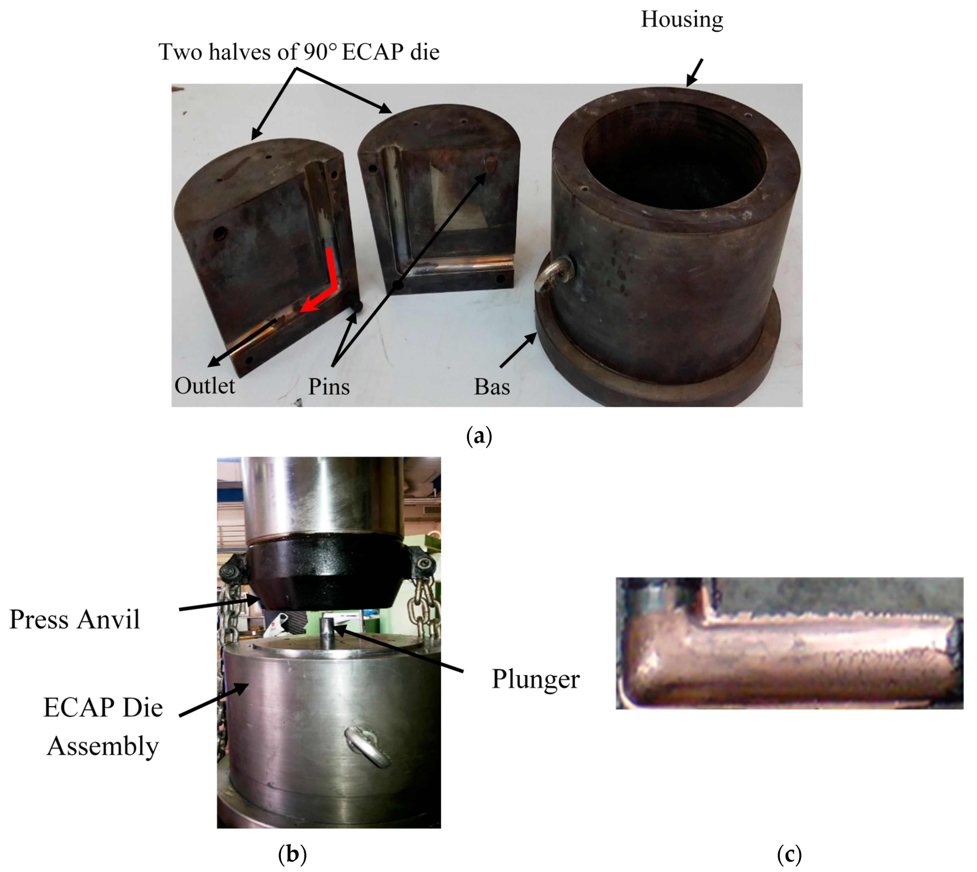
ECAP was applied by using a 90° channel die made from H13 steel. Four passes of ECAP (route BC) at room temperature were completed using a hydraulic press with a capacity of 160 tons. During the ECAP process, MoS2 was used to reduce the friction between the sample and the die walls. Figure 1 shows the setup of the ECAP process.
2.2. Erosion-Corrosion Experiments
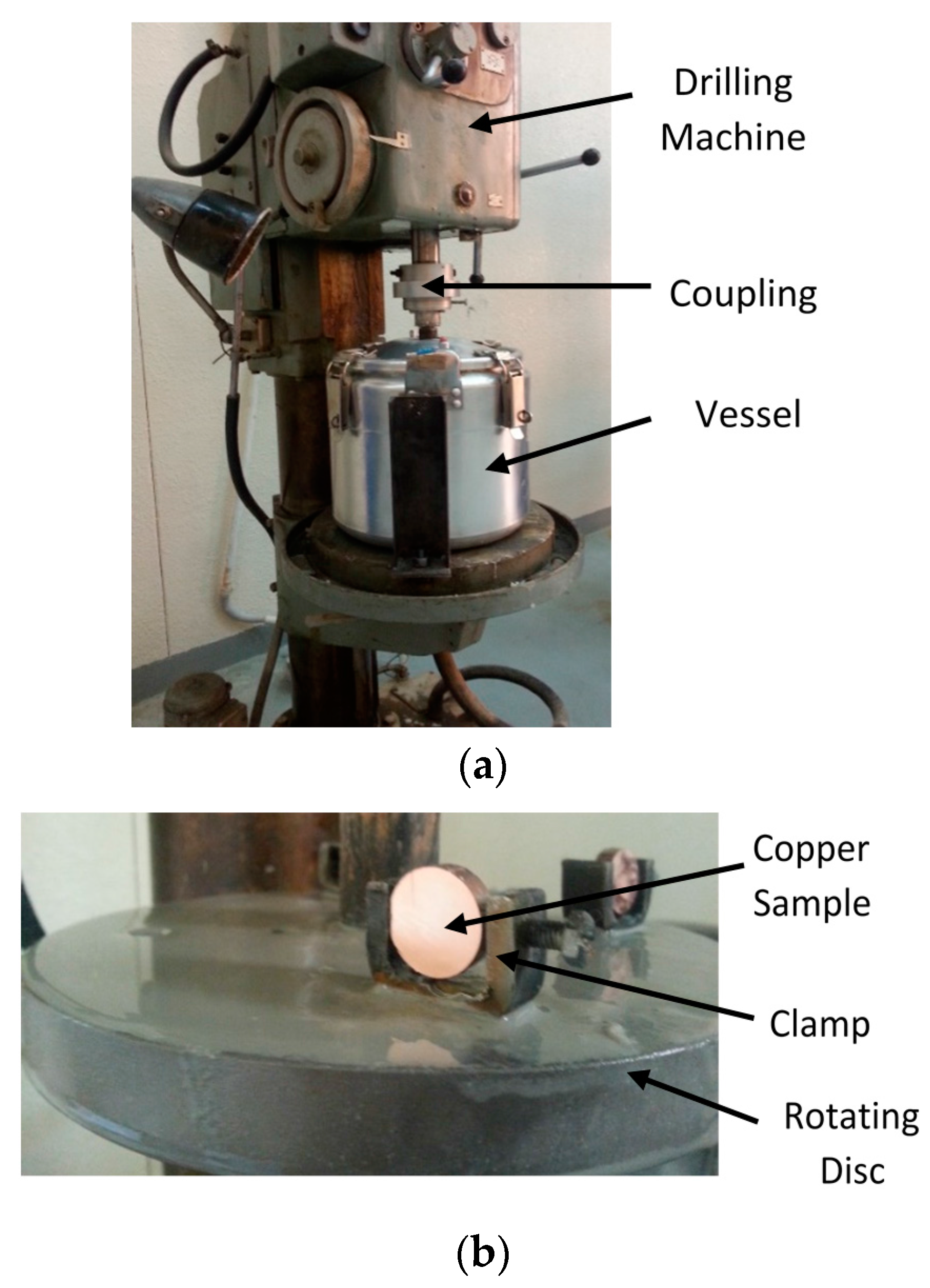
The slurry pot method was employed to examine the E-C behavior of standard and nanostructured pure copper. The copper specimens were cut into smaller samples that were 20 mm in diameter and 6 mm in thickness. A slurry solution containing 3.5% NaCl—to provide the corrosion effect—and solid particles (SiO2 ranging from 300 μm to 500 μm in size)—to provide the erosion effect—were used in the experiments. The slurry was contained within a cylindrical vessel with a diameter of 300 mm and a height of 350 mm, as shown in Figure 2a. The E-C samples were clamped to a circular disc at different radial distances to achieve a variety of linear speeds when revolving in the slurry (see Figure 2b). The disc was bolted to a shaft that was attached to the spindle of a drilling machine by an aluminum rigid coupling. Each test was repeated twice, and the average mass loss per unit area was computed.
3. Results and Discussion
3.1. Comparison of E-C for Coarse and Nanostructured Grain COPPER
To validate the reduction of grain size, the grain size of both annealed ECAPed samples was measured. The optical (annealed) and Scanning Electron Microscopy (SEM) (4 pass ECAP) microstructures of the commercial pure copper are shown in Figure 3. Approximately, a 100% reduction in grain size was observed after the ECAP process. The average grain size before and after ECAP was 1000 nm and 600 nm respectively.
Using the previously described procedures, experiments were conducted to compare the E-C on standard (coarse) and nanostructure copper under various conditions. The objective of these comparisons was to investigate any improvements in the E-C resistance of copper resulting from the ECAP. In particular, the effect of impact velocity, time, and erodent concentration were studied, as discussed in the following subsections.
3.1.1. Impact Velocity Effect
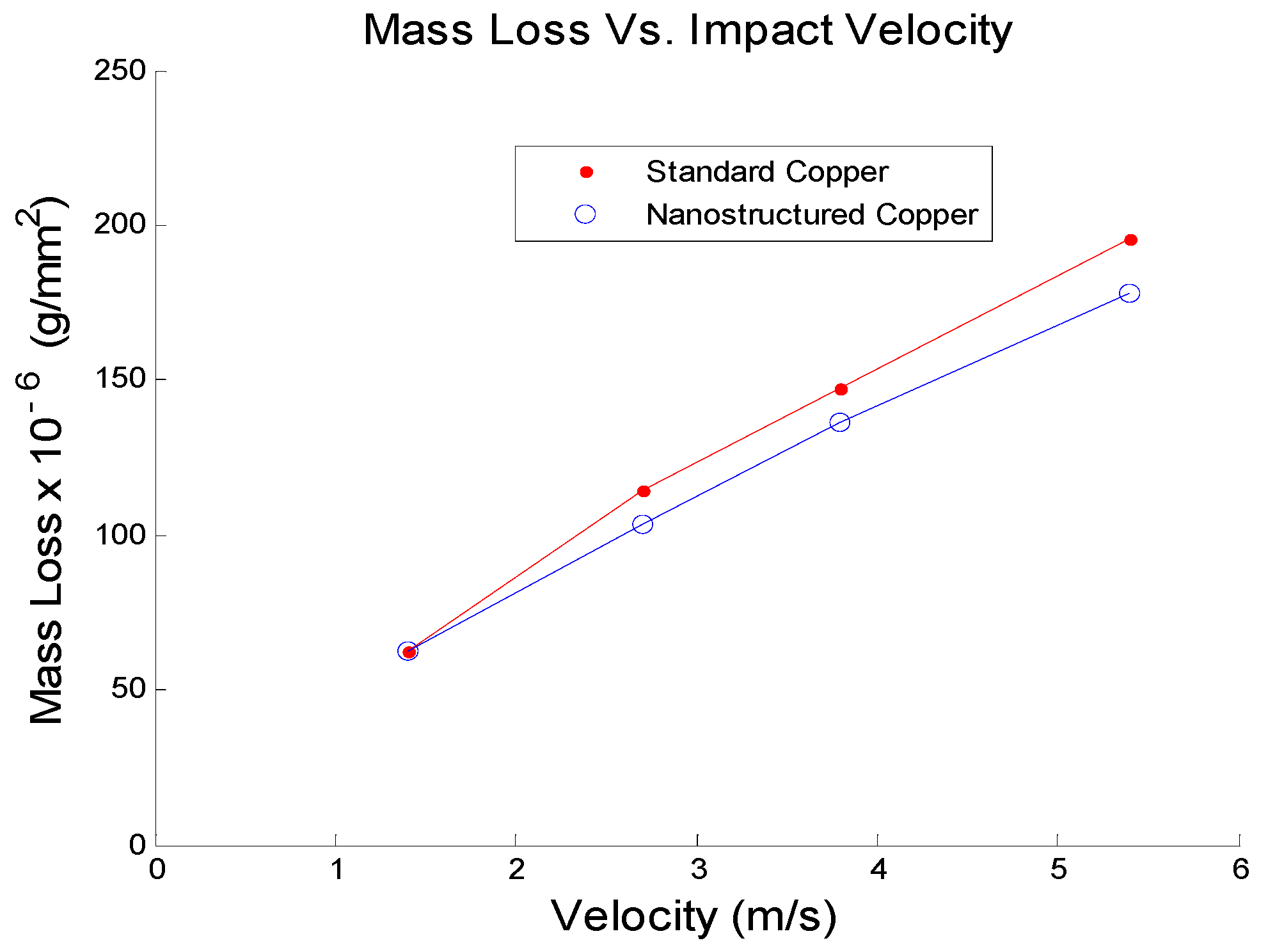
Erosion–Corrosion experiments were performed on both standard (coarse) and nanostructured copper for four velocity settings, namely 1.4 m/s, 2.7 m/s, 3.8 m/s, and 5.4 m/s. The testing time and erodent (sand) concentration were kept at 48 h and 20%, respectively. The graph in Figure 4 shows a comparison of the E-C between the standard and nanostructured copper for the various velocities.
3.1.2. Time Effect
The effect of time on the E-C of both the coarse and nanostructured copper samples was studied for various testing times, namely 12 h, 24 h, and 48 h. For all three-test durations, the impact velocity was kept constant at 3.8 m/s, while the erodent (sand) concentration was kept at 20%. In Figure 5, a comparison of the E-C between the standard and nanostructured copper for the various test durations is shown.
3.1.3. Erodent Concentration Effect
In addition, E-C experiments were performed on both the coarse and nanostructured copper for various sand concentrations. Four concentration levels were considered, namely 0%, 10%, 20%, and 30%. For all concentration levels, the testing time was kept at 48 h and the impact velocity was kept at 3.8 m/s. The graph in Figure 6 shows a comparison of the E-C between the standard and nanostructured copper for the various concentration levels.
3.2. Combined Effect of Time, Impact Velocity, and Erodent Concentration on E-C of Nanostructured Copper
Experiments were carried out to investigate the combined effect of time, impact velocity, and erodent (sand) concentration on the E-C of nanostructured copper, as presented in the following subsections.
3.2.1. Data Points for the Experiments
E-C experiments are extremely expensive because there is a need for advanced planning with regard to the reservation of equipment, facilities, and skilled technicians, as well as substantial setup and running times. In the current work, the situation is further exacerbated because the specimens (i.e., nanostructured ECAP copper) are difficult and time-consuming to manufacture. For these reasons, the combinations of data points for the experiments should be carefully designed to cover the test variables (i.e., test time, impact velocity, and sand concentration). In addition, the choice of data points for which the experiments will be performed has a large effect on the quality of the surface fit that will be used to generate the surface plots that enable the visualization of the combined effects of the test variables on the E-C behavior of nanostructured ECAP copper.
The combination of points at which the tests will be performed can be selected using the design of experiments (DOE) procedure. Angela and Voss [43] and Oehlert [44] provide in-depth descriptions of the methodology. In this work, the popular central composite design (CCD)—namely, the face-centered approach—is used. The domain for the test variables is simply defined by the lower and upper limits, resulting in a regular boxlike domain. Table 2 shows the lower and upper bounds for the three variables. The impact velocity is limited by the experimental equipment in this work, but its bounds are nonetheless similar to what is found in the literature [45,46]. The bounds of the sand concentration and testing time are also based on the literature [47].
With the stated bounds, the combination of test points for the experiment can be determined based on the face-centered CCD. The fifteen combinations of test points generated using this DOE are listed in Table 3, including eight corner points (Tests 1–8), six axial points (Tests 9–14), and one central point (Test 15).
The E-C experiments were conducted according to the combinations of test points listed in Table 3. In order to alleviate the cost associated with the experiments (as both ECAP and the E-C testing process are expensive), it should be noted that although 15 different combinations of variables are stated, fewer than 15 samples can be used if the experiments are well planned. For example, Tests 1 and 5 can utilize the same sample as only the time is varying (other quantities are constant); thus, after 10 h, the test sample can be measured to determine the extent of E-C. The same specimen can then be used to complete Test 5. This procedure can therefore be used to reduce the costs with regard to the number of specimens used and the total experimental time. The results from the experiments are listed in Table 4. For each of the combinations of test points, two tests were conducted and the mean of the two values was recorded. It is worth noting that conducting several experiments for each of the combinations of test points (to obtain a proper average) would be too expensive and therefore infeasible.
3.2.2. Surface Fitting
In order to visualize and interpret the results in Table 4, the surfaces were fit to the data, from which surface plots were generated. Surface plots were generated using two techniques: polynomial regression and Kriging. What follows are brief descriptions and the results of the two approaches.
Polynomials Regression
In the first approach, surface plots are generated using polynomials. Least squares regression was used to fit the data with first- and second-order polynomials, of the forms in Equations (1) and (2), respectively:
where w is the mass loss per unit area; t, v, and s are the test variables (time, impact velocity, and sand concentration, respectively); and represents the coefficients to be determined. The two polynomials were constructed in an effort to reveal the trends of the data. Chapra and Canale [48] provide a detailed discussion of the regression models, determination of the coefficients, and model evaluation for quality of fit.
In Table 5, the coefficient of determination for the first- and second-order polynomials are reported as 0.8444 and 0.9863, respectively. In addition, the value of the coefficient of determination for the second-order polynomial (0.9863) indicates that the quadratic polynomial was a reasonably good fit. Therefore, within the domain of the data, its can reasonably be stated that the trend is quadratic rather than linear.
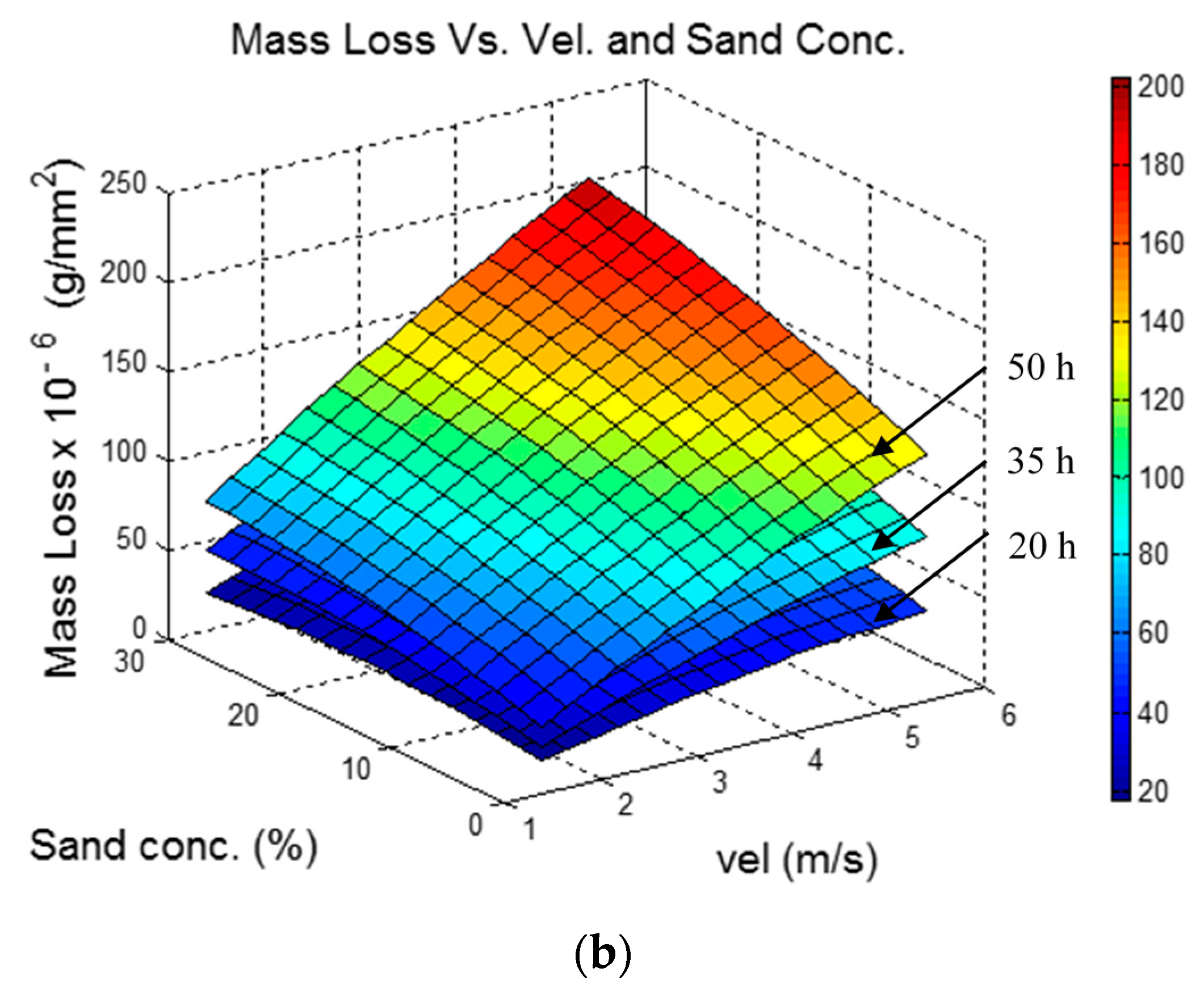
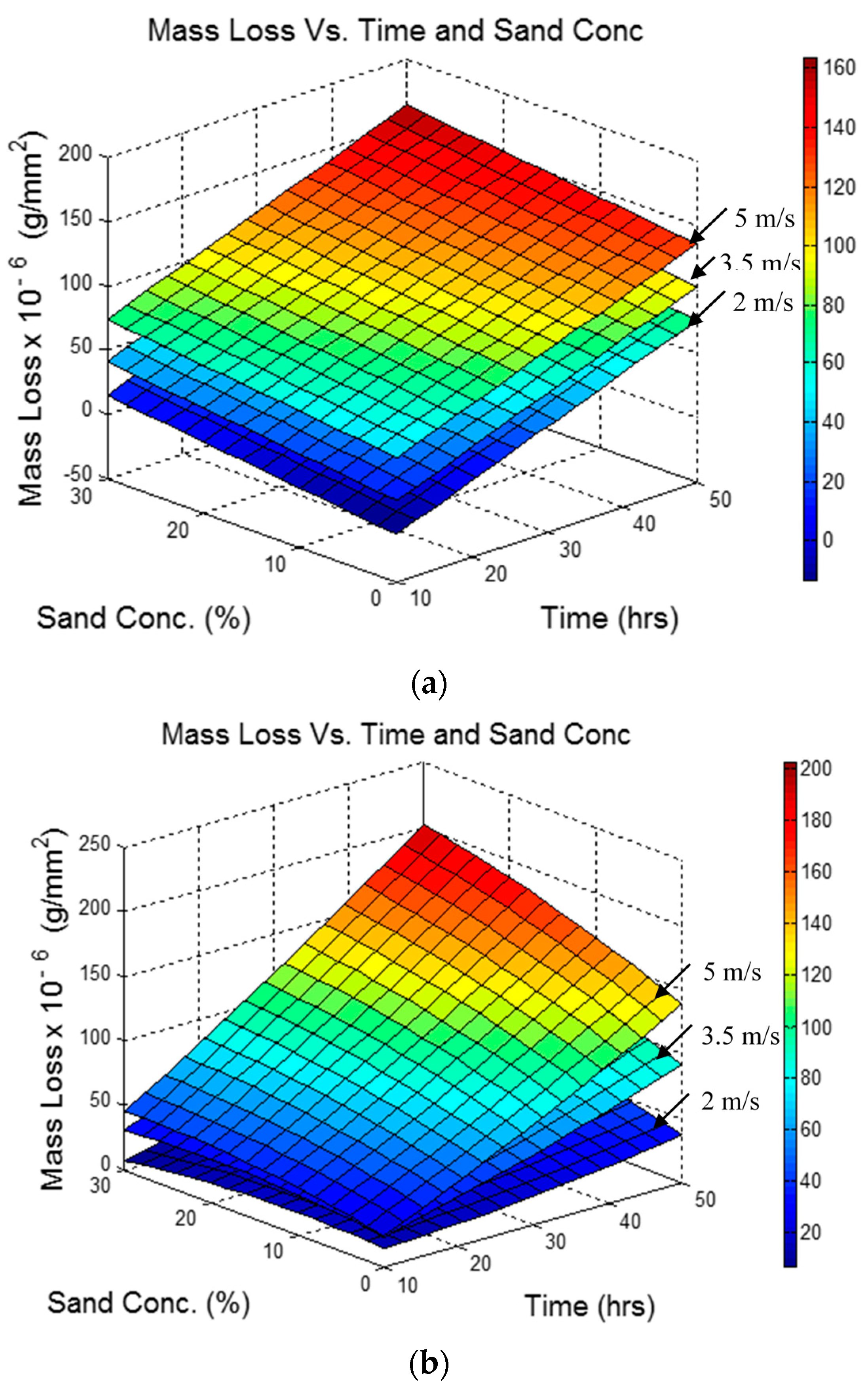
Using Equations (1) and (2), surface plots were generated to reveal the combined effect of time, velocity, and sand concentration on the E-C of nanostructured ECAP copper for both the linear and quadratic polynomials (for comparison). In Figure 7, the mass loss is plotted as a function of sand concentration and velocity for various times (specified in the figure). In Figure 8, the mass loss is plotted as a function of time and sand concentration for various velocities. In Figure 9, the mass loss is plotted as a function of time and velocity for various sand concentrations.
Kriging was used as an alternative approach to establish the relation between the mass loss, testing time, impact velocity, and sand concentration. Kriging was initially developed by geologists as a means to approximate the properties of minerals within a region of interest based on the information of mineral properties in other regions [49]. It is an interpolation technique based on regression against observed values of neighboring data points that are weighted according to spatial covariance values. The equation for Kriging has the following form [49,50]:
The first part of the equation, , is a regression model consisting of a linear combination of q regressors (i.e., chosen functions such as polynomials). This part models the trend of the domain. The second part of Equation (3), , is a random process assumed to have a mean of zero and a covariance described as:
In Equation (4), the process variance, , has the effect of scaling the spatial correlation function, . It is worth noting that the correlation function is responsible for the smoothness of the final Kriging model, whereas the second part of Equation (3) is considered as having the effect of pulling the response over the data by quantifying the correlation of neighboring data points [49]. More detailed information on the application of Kriging and a determination of the mean square errors (MSE) (measure of quality of an estimator) can be found in the references [49,50].
In this work, the Kriging form and Kriging Matlab toolbox were employed [50]. The toolbox offers the options of zeroth-, first-, and second-order polynomials for the regression model. In the current study, first- and second-order polynomials were used, and the resulting surface plots are compared. Several correlation models, such as gauss, exponential, spherical, spline, cubic, and linear, are available for use in the toolbox. The spline correlation model was selected for this work.
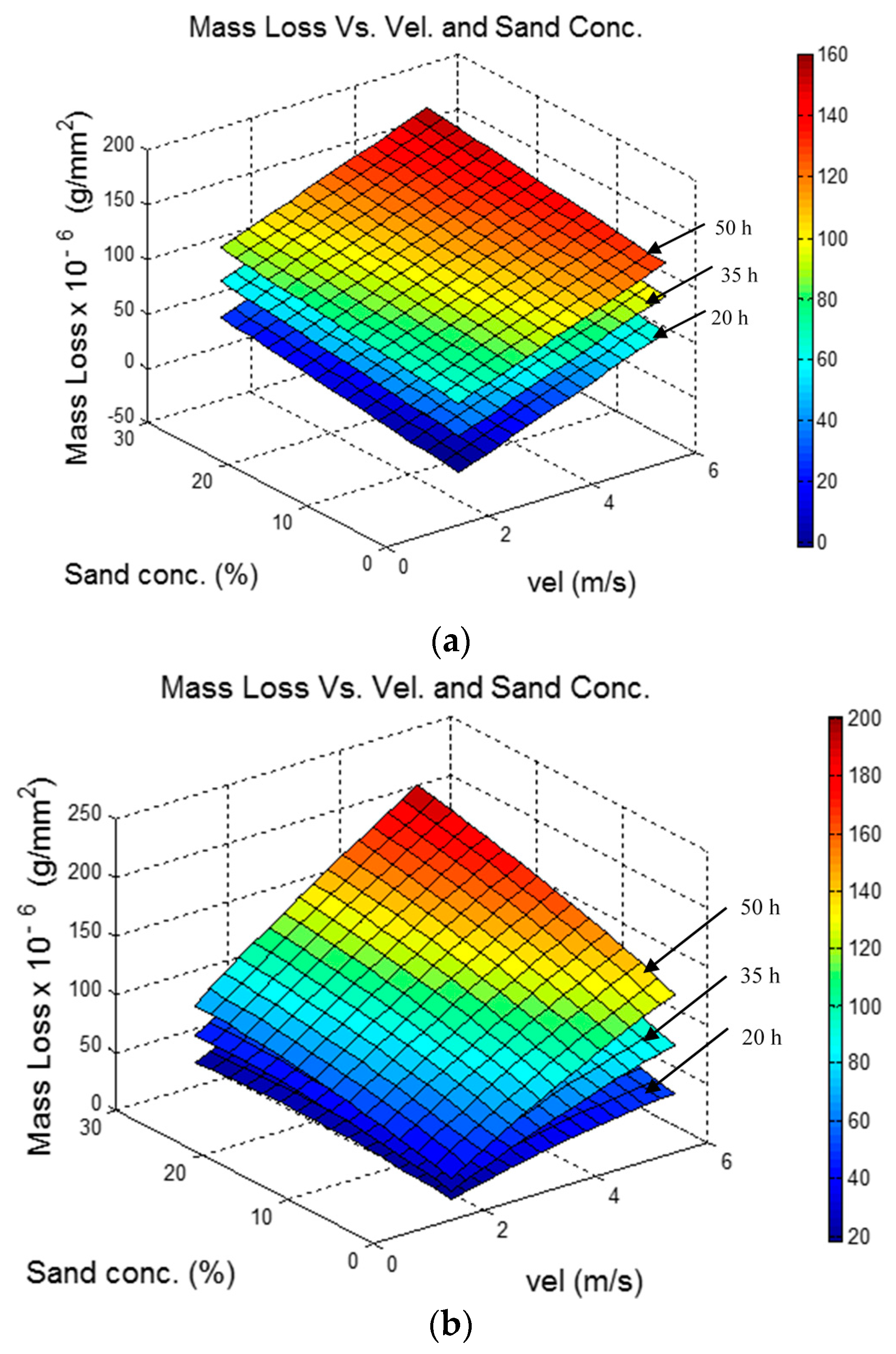
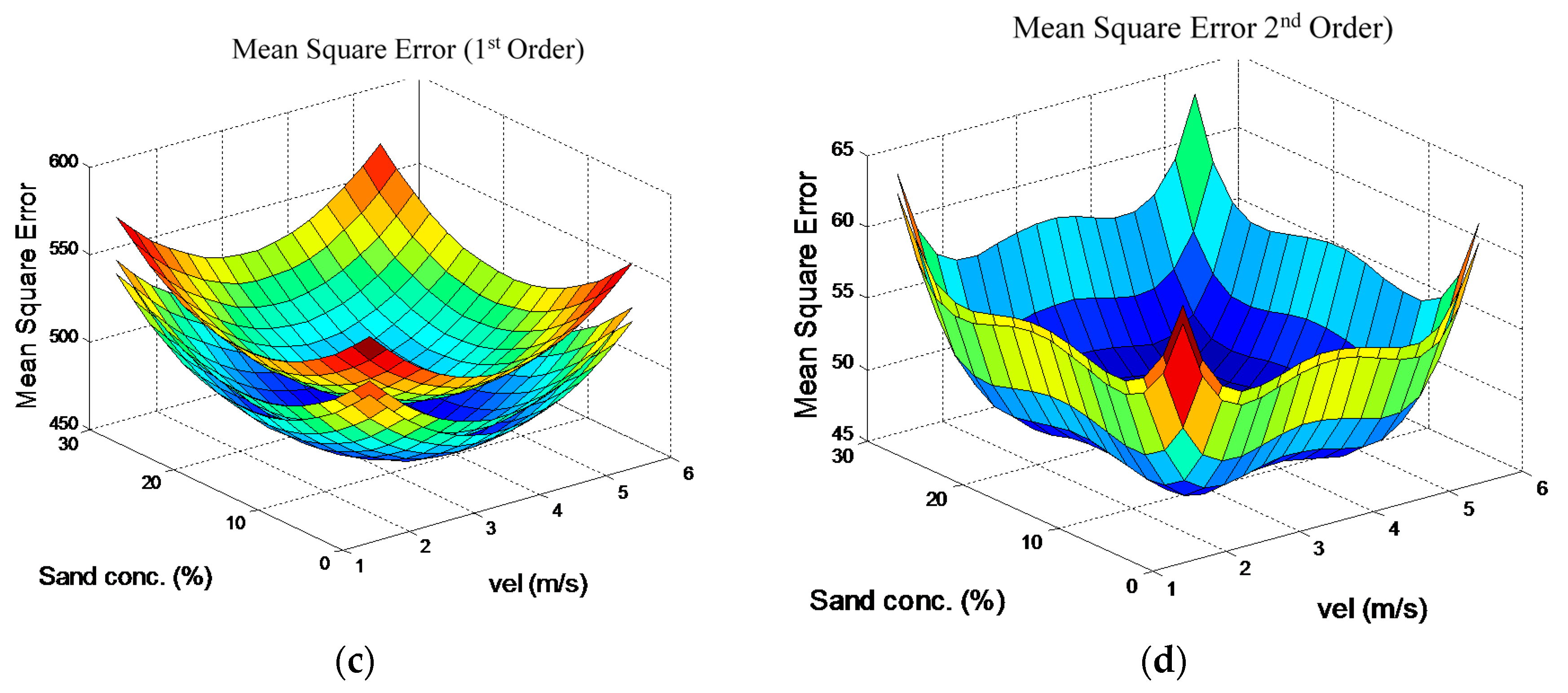
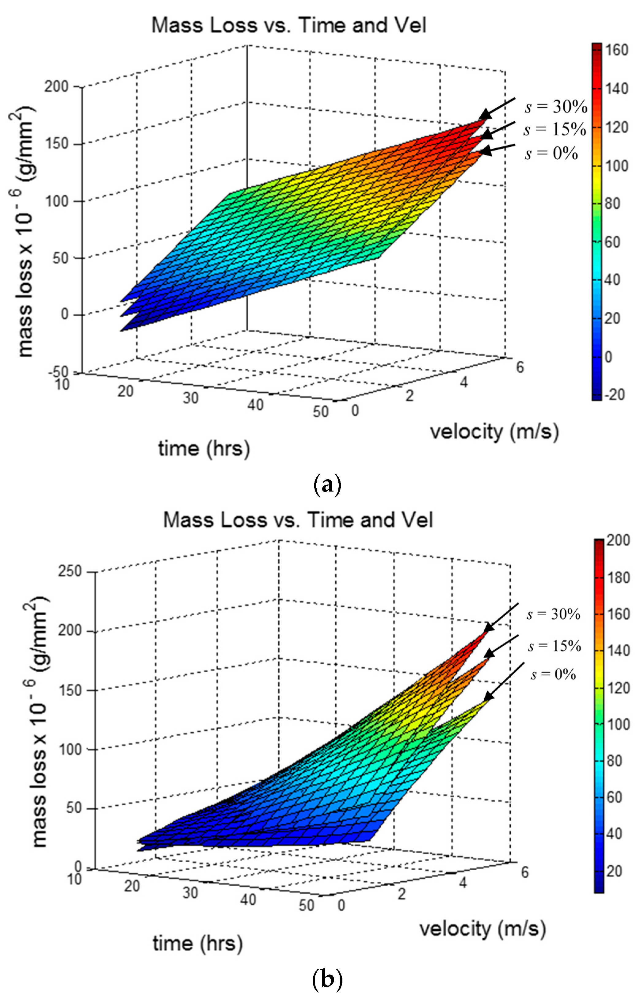
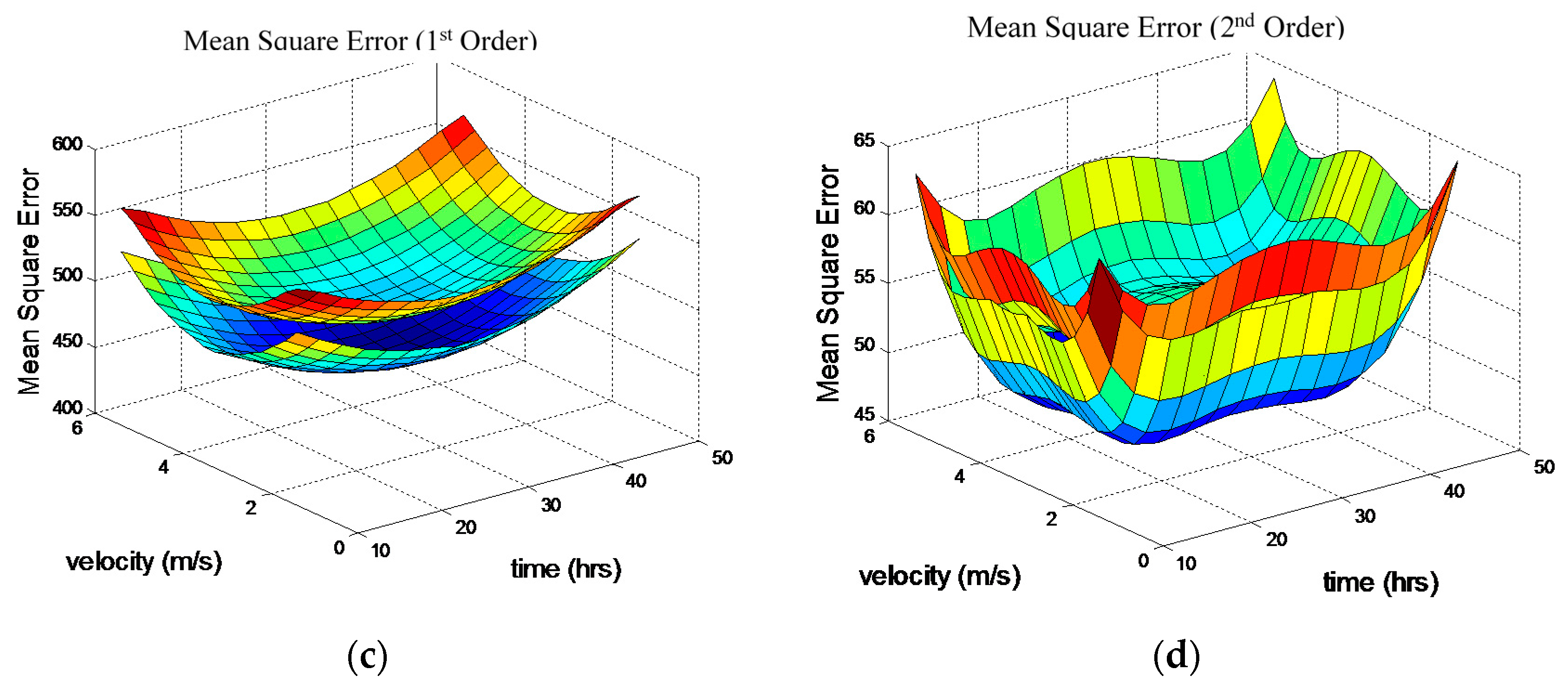
Utilizing data from Table 4, surface plots were generated using the Kriging approach. In Figure 10, the mass loss as a function of sand concentration and velocity is plotted for various times (specified in the figure) for both the first- and second-order models. In addition, the MSE of the first- and second-order models are also plotted for comparison. In Figure 11, the mass loss is plotted as a function of time and sand concentration for various velocities; in Figure 12, the mass loss is plotted as a function of time and velocity for various sand concentrations. As in Figure 10, Figure 11 and Figure 12, the MSE corresponding to the first- and second-order models are also plotted and compared.
3.3. Discussion
Figure 4, Figure 5 and Figure 6, respectively, show the effect of impact velocity, testing time, and sand concentration on the E-C of standard (coarse) and nanostructured copper. The three figures indicate that any increase of the individual test parameters (impact velocity, testing time, and sand concentration) results in higher E-C on both the standard and nanostructured copper. In addition, it can be seen, that as the individual parameters are increased, the amount of E-C on the nanostructured copper was increasingly less than what was observed on the coarse copper. It can thus be stated that, under the studied conditions, nanostructured copper is more superior in resisting E-C than standard copper.
From the six figures (Figure 7, Figure 8, Figure 9, Figure 10, Figure 11 and Figure 12), a number of observations can be made regarding the effects of testing time, velocity, and sand concentration on the E-C behavior of nanostructured copper. These observations are discussed in the following subsections.
3.3.1. Trend of the Surface
Within the domain of the test data, the mass loss due to the E-C of nanostructured ECAP copper is best described by a quadratic function of time, velocity, and sand concentration. In the case of the polynomial regression, it is clear from the coefficients of determination (see Table 5) of the linear polynomial (r2 = 0.844) and the quadratic polynomial (r2 = 0.986) that the quadratic function is a better fit. Similarly, in the Kriging approach, the MSE for the three sets of surface plots (Figure 10c,d, Figure 11c,d, and Figure 12c,d) also reveal that the most appropriate model is the 2nd order model because the values of the MSE obtained for the first-order model are very high in all three sets of surface plots. Thus, from the two approaches, it can be stated with reasonable confidence that the trend of the data is quadratic.
3.3.2. Effect of Testing Time, Impact Velocity, and Sand Concentration
From Figure 8b and Figure 11b, it is observed that for a specific value of sand concentration (e.g., a low concentration of 0%), the mass loss increases with an increasing testing time. For greater sand concentrations (e.g., 30%), the mass loss is more rapid. In Figure 7b and Figure 10b, it can be observed that the mass loss increases with an increasing sand concentration, and increases for a given velocity and testing time (e.g., 2 m/s and 50 h). This is also true for higher velocities (e.g., 5 m/s), except that the mass loss is more rapid as the sand concentration increases. Thus, an increased impact velocity enhances the effect of sand concentration on mass loss. This increase in mass loss relative to sand concentration is consistent with other studies [30,31,33]. It can also be observed that the amount of mass loss increases with testing time regardless of the sand concentration, as long as the impact velocity is greater than zero (See Figure 7b and Figure 11b for 0% sand concentration). From Figure 9b and Figure 12b, it is noted that for a specific value of the testing time (e.g., 50 h), the mass loss increases with an increasing impact velocity. This observation is consistent with observations in previous studies [30,33].
Finally, the surface plots based on polynomial regression (Figure 7b, Figure 8b and Figure 9b) and Kriging (Figure 10b, Figure 11b and Figure 12b) reveal that the synergetic effect of the three parameters (testing time, impact velocity, and sand concentration) on the E-C behavior of nanostructured ECAP copper is much greater than the effect of each individual parameter.
4. Conclusions
Tests were performed on standard and nanostructured copper to investigate their E-C behavior under specified conditions for three test parameters, namely impact velocity, testing time, and erosive solid particle (sand) concentration. It was established that nanostructured copper is more superior in terms of resisting E-C than traditional standard copper.
In a separate set of tests, nanostructured ECAP copper was subjected to E-C tests to study the combined effect of three parameters: testing time, impact velocity, and erosive solid particle concentrations. The E-C tests were conducted on selected test points within the defined domain of the test parameters. Surface plots were generated from the test results, from which the following conclusions can be drawn:
- The E-C of nanostructured copper is better described by a quadratic function of the testing time, impact velocity, and sand concentration than a linear function.
- The E-C of nanostructured copper increases with an increasing testing time, impact velocity, and sand concentration.
- Mass loss due to E-C is more severe for higher impact velocities. This possibly occurs because the increased velocity raises the impact energy of the sand particles on the test specimen and the reaction rate with the corrosive agent, thus accelerating the mass loss.
- The polynomial regression and Kriging techniques were effective in fitting the surfaces to the experimental data to allow for a visualization of the trends. For the polynomial regression, the coefficient of determination was 0.986, indicating a good fit for the second-order polynomial. In the case of the Kriging approach, the MSE for the quadratic model were found to be much lower than those of the linear model, further strengthening the argument that the trend is quadratic.
- Simultaneously increasing the three test parameters (testing time, impact velocity, and sand concentration) causes a more significant increase in the E-C of nanostructured copper than the sum of individually increasing each parameter.
Acknowledgments
The authors gratefully acknowledge Qassim University, represented by the Deanship of Scientific Research, for the material support for this research under grant number 3027 during the academic year 1437–1438 H–2015–2016 G.
Author Contributions
Osama M. Irfan and Saad M. S. Mukras designed and performed the experiments and analyzed the data. They also participated in writing the paper. Fahad A. Al-Mufadi contributed in analyzing the data and Faramarz Djavanroodi was project supervisor and wrote the paper.
Conflicts of Interest
The authors declare no conflict of interest.
References
- Yang, Y.; Cheng, Y.F. Parametric effects on the erosion-corrosion rate and mechanism of carbon steel pipes in oil sands slurry. Wear 2012, 276–277, 141–148. [Google Scholar] [CrossRef]
- Tian, B.R.; Cheng, Y.F. Erosion–corrosion of hydro-transport pipes in oil sand slurries. Bull. Electrochem. 2006, 22, 329–335. [Google Scholar]
- Tian, B.R.; Cheng, Y.F. Electrochemical corrosion behavior of X-65 steel in the simulated oil sand slurry. I: Effects of hydrodynamic condition. Corros. Sci. 2008, 50, 773–779. [Google Scholar] [CrossRef]
- Zhang, G.A.; Cheng, Y.F. Electrochemical corrosion of X65 pipe steel in oil/water emulsion. Corros. Sci. 2009, 51, 901–907. [Google Scholar] [CrossRef]
- Tian, B.R.; Cheng, Y.F. Electrolytic deposition of Ni–Co–Al2O3 composite coating on pipe steel for corrosion/erosion resistance in oil sand slurry. Electrochim. Acta 2007, 53, 511–517. [Google Scholar] [CrossRef]
- Guo, H.X.; Lu, B.T.; Luo, J.L. Interaction of mechanical and electrochemical factors in erosion-corrosion of carbon steel. Electrochim. Acta 2005, 51, 315–323. [Google Scholar] [CrossRef]
- Neville, A.; Reza, F.; Chiovelli, S.; Revega, T. Erosion–corrosion behaviour of WC based MMCs in liquid-solid slurries. Wear 2005, 259, 181–195. [Google Scholar] [CrossRef]
- Kamdi, Z.; Shipway, P.H.; Voisey, K.T.; Sturgeon, A.J. Abrasive wear behavior of conventional and large-particle tungsten carbide-based cermet coatings as a function of abrasive size and type. Wear 2011, 271, 1264–1272. [Google Scholar] [CrossRef]
- Hussain, E.A.M.; Robinson, M.J. Erosion–corrosion of 2205 duplex stainless steel in flowing seawater containing sand particles. Corros. Sci. 2007, 49, 1737–1754. [Google Scholar] [CrossRef]
- Neville, A.; Hodgkiess, T.; Xu, H. An electrochemical and microstructural assessment of erosion-corrosion of cast-iron. Wear 1999, 233–235, 523–534. [Google Scholar] [CrossRef]
- Clark, H.M. The influence of flow field in slurry erosion. Wear 1992, 152, 223–240. [Google Scholar] [CrossRef]
- Souza, V.A.D.; Neville, A. Aspects of microstructure on the synergy and overall material loss of thermal spray coatings in erosion-corrosion environments. Wear 2007, 263, 339–346. [Google Scholar] [CrossRef]
- Stack, M.M.; Pungwiwat, N. Particulate erosion-corrosion of Al in aqueous conditions: Some perspectives on pH effects on the erosion–corrosion map. Tribol. Int. 2002, 35, 651–660. [Google Scholar] [CrossRef]
- Neville, A.; Reyes, M.; Xu, H. Examining corrosion effects and corrosion/erosion interactions on metallic materials in aqueous slurries. Tribol. Int. 2002, 35, 643–650. [Google Scholar] [CrossRef]
- Quddus, A.; Al-Hadrami, L.M. Influence of solution hydrodynamics on the deposition of CaSO4 scale on aluminum. J. Thermophys. Heat Transf. 2011, 25, 112–118. [Google Scholar] [CrossRef]
- Maciel, J.M.; Agostinho, S.M.L. Use of a rotating cylinder electrode in corrosion studies of a 90/10 Cu–Ni alloy in 0.5 mol·L−1 H2SO4 media. J. Appl. Electrochem. 2000, 30, 981–985. [Google Scholar] [CrossRef]
- Novák, P.; Macenauer, A. Erosion-corrosion of passive metals by solid particles. Corros. Sci. 1993, 35, 635–640. [Google Scholar] [CrossRef]
- Hong, T.; Jepson, W.P. Corrosion inhibitor studies in large flow loop at high temperature and high pressure. Corros. Sci. 2001, 43, 1839–1849. [Google Scholar] [CrossRef]
- Hassani, S.; Roberts, K.P.; Shirazi, S.A.; Shadley, J.R.; Rybicki, E.F.; Joia, C. Characterization and prediction of chemical inhibition performance for erosion-corrosion conditions in sweet oil and gas production. Corrosion 2012, 68, 885–896. [Google Scholar] [CrossRef]
- Rihan, R.O.; Nešić, S. Erosion-corrosion of mild steel in hot caustic. Part I: NaOH solution. Corros. Sci. 2006, 48, 2633–2659. [Google Scholar] [CrossRef]
- Islam, M.A.; Farhat, Z.N. Mechanical and electrochemical synergism of API X42 pipeline steel during erosion-corrosion. J. Bio- Tribo-Corros. 2015, 1, 26. [Google Scholar] [CrossRef]
- Koike, M.H. Erosion-corrosion of stainless steel pipes under two-phase flow with steam quality 26%. J. Nucl. Mater. 2005, 342, 125–130. [Google Scholar] [CrossRef]
- Sasaki, K.; Burstein, G.T. Erosion-corrosion of stainless steel under impingement by a fluid jet. Corros. Sci. 2007, 49, 92–102. [Google Scholar] [CrossRef]
- Mitelea, I.; Micu, L.M.; Bordeaşu, I.; Crăciunescu, C.M. Cavitation erosion of sensitized UNS S31803 duplex stainless steels. J. Mater. Eng. Perform. 2016, 25, 1939–1944. [Google Scholar] [CrossRef]
- Wang, Q.Y.; Bai, S.L.; Liu, Z.D. Surface characterization and erosion-corrosion behavior of Q235 steel in dynamic flow. Tribol. Lett. 2014, 53, 271–279. [Google Scholar] [CrossRef]
- Dular, M.; Osterman, A. Pit clustering in cavitation erosion. Wear 2008, 265, 811–820. [Google Scholar] [CrossRef]
- Rajahram, S.S.; Harvey, T.J.; Wood, R.J.K. Erosion-corrosion resistance of engineering materials in various test conditions. Wear 2009, 267, 244–254. [Google Scholar] [CrossRef]
- Burstein, G.T.; Sasaki, K. Effect of impact angle on slurry erosion-corrosion of 304L stainless steel. Wear 2000, 240, 80–94. [Google Scholar] [CrossRef]
- Abbade, N.P.; Crnkovic, S.J. Sand-water slurry erosion of API 5L X65 pipe steel as quenched from intercritical temperature. Tribol. Int. 2000, 33, 811–816. [Google Scholar] [CrossRef]
- Meng, H.; Hu, X.; Neville, A. A systematic erosion-corrosion study of two stainless steels in marine conditions via experimental design. Wear 2007, 263, 355–362. [Google Scholar] [CrossRef]
- Nawale, E.A.; Mohammed, A.A.; Sondus, M. Study the effect of erosion-corrosion of Al-Mg-Si alloy in marine environment. Eng. Technol. J. 2013, 31, 254–264. [Google Scholar]
- Wang, L.; Qiu, N.; Hellmann, D.H.; Zhu, X. An experimental study on cavitation erosion-corrosion performance of ANSI 1020 and ANSI 4135 steel. J. Mech. Sci. Technol. 2016, 30, 533–539. [Google Scholar] [CrossRef]
- Irfan, O.M.; El-Nasr, A.A.; Al-Mufadi, F. Erosion-corrosion behaviour of AA 6066 aluminium alloy. Int. J. Mech. Eng. 2014, 3, 15–24. [Google Scholar]
- Irfan, O.M. Erosion-corrosion behavior of nano-structured pure copper under different flowing velocities. Int. J. Mech. Mechatron. Eng. 2015, 15, 48–52. [Google Scholar]
- Sakamoto, A.; Yamasaki, T.; Matsumura, M. Erosion-corrosion tests on copper alloys for water tap use. Wear 1995, 186–187, 548–554. [Google Scholar] [CrossRef]
- Ebrahimi, M.; Djavanroodi, F. Experimental and numerical analyses of pure copper during ECFE process as a novel severe plastic deformation method. Prog. Nat. Sci. 2014, 24, 68–74. [Google Scholar] [CrossRef]
- Hosseini, E.; Kazeminezhad, M. The effect of ECAP die shape on nano-structure of materials. Comput. Mater. Sci. 2009, 44, 962–967. [Google Scholar] [CrossRef]
- Shaeri, M.H.; Shaeri, M.; Salehi, M.T.; Seyyedein, S.H.; Djavanroodi, F. Microstructure and texture evolution of Al-7075 alloy processed by equal channel angular pressing. Trans. Nonferr. Met. Soc. China 2015, 25, 1367–1375. [Google Scholar] [CrossRef]
- Azushima, A.; Kopp, R.; Korhonen, A.; Yang, D.Y.; Micari, F.; Lahoti, G.D.; Groche, P.; Yanagimoto, J.; Tsuji, N.; Rosochowski, A.; et al. Severe plastic deformation (SPD) processes for metals. CIRP Ann. Manuf. Technol. 2008, 57, 716–735. [Google Scholar] [CrossRef]
- Šedivý, O.; Beneš, V.; Ponížil, P.; Král, P.; Sklenička, V. Quantitative characterization of microstructure of pure copper processed by ECAP. Image Anal. Stereol. 2013, 32, 65–75. [Google Scholar] [CrossRef]
- Kumar, M.; Singh, H.; Singh, N.; Chavan, N.M.; Kumar, S.; Joshi, S.V. Development of erosion-corrosion-resistant cold-spray nanostructured Ni–20Cr coating for coal-fired boiler applications. J. Therm. Spray Technol. 2015, 24, 1441–1449. [Google Scholar] [CrossRef]
- Kumar, M.; Singh, H.; Singh, N.; Joshi, R.S. Erosion–corrosion behavior of cold-spray nanostructured Ni–20Cr coatings in actual boiler environment. Wear 2015, 332–333, 1035–1043. [Google Scholar] [CrossRef]
- Dean, A.M.; Voss, D. Design and Analysis of Experiments; Springer: New York, NY, USA, 1999. [Google Scholar]
- Oehlert, G.W. A First Course in Design and Analysis of Experiments. 2010. Available online: http://hdl.handle.net/11299/168002 (accessed on 3 December 2016).
- Wood, R.J.K. Erosion-corrosion interactions and their effect on marine and offshore material. Wear 2006, 261, 1012–1023. [Google Scholar] [CrossRef]
- Barik, R.C.; Wharton, J.A.; Wood, R.J.K.; Tan, K.S.; Stokes, K.R. Erosion and erosion-corrosion performance of cast and thermally sprayed nickel–aluminium bronze. Wear 2005, 259, 230–242. [Google Scholar] [CrossRef]
- Sasaki, K.; Burstein, G.T. The generation of surface roughness during slurry erosion-corrosion and its effect on the pitting potential. Corros. Sci. 1996, 38, 2111–2120. [Google Scholar] [CrossRef]
- Chapra, S.C.; Canale, R.P. Numerical Methods for Engineers, 7th ed.; McGraw-Hill: New York, NY, USA, 2014. [Google Scholar]
- Martin, J.D.; Simpson, T.W. Use of Kriging models to approximate deterministic computer models. AIAA J. 2005, 43, 853–863. [Google Scholar] [CrossRef]
- Lophaven, S.N.; Nielsen, H.B.; Søndergaard, J. DACE: A MATLAB Kriging Toolbox Version 2.0; Technical Report IMM-TR-2002-12; Technical University of Denmark: Lyngby, Denmark, 2002. [Google Scholar]
Figure 1.
Setup of ECAP process; (a) Details of ECAP die; (b) Pressing; (c) Copper sample after four ECAP passes.
Figure 1.
Setup of ECAP process; (a) Details of ECAP die; (b) Pressing; (c) Copper sample after four ECAP passes.

Figure 2.
Setup of E-C test by slurry pot method; (a) Setup assembly; (b) Copper samples clamped to rotating disc.
Figure 2.
Setup of E-C test by slurry pot method; (a) Setup assembly; (b) Copper samples clamped to rotating disc.

Figure 3.
The Optical and SEM microstructure of annealed and nanostructure copper. (a) Annealed coarse grained copper; (b) Nanostructured copper.
Figure 3.
The Optical and SEM microstructure of annealed and nanostructure copper. (a) Annealed coarse grained copper; (b) Nanostructured copper.
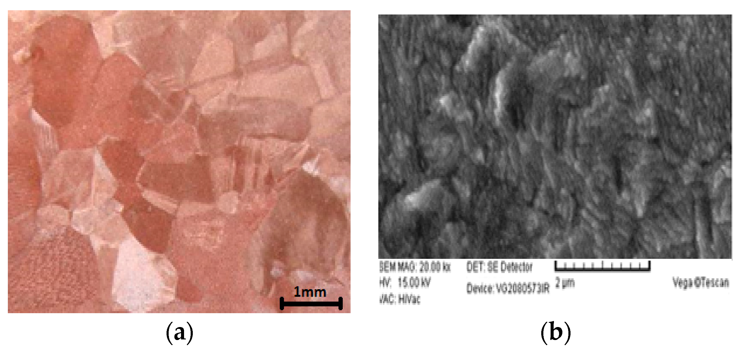
Figure 4.
Mass loss versus velocity for both standard and nanostructure copper.

Figure 5.
Mass loss versus time for both standard and nanostructure copper.
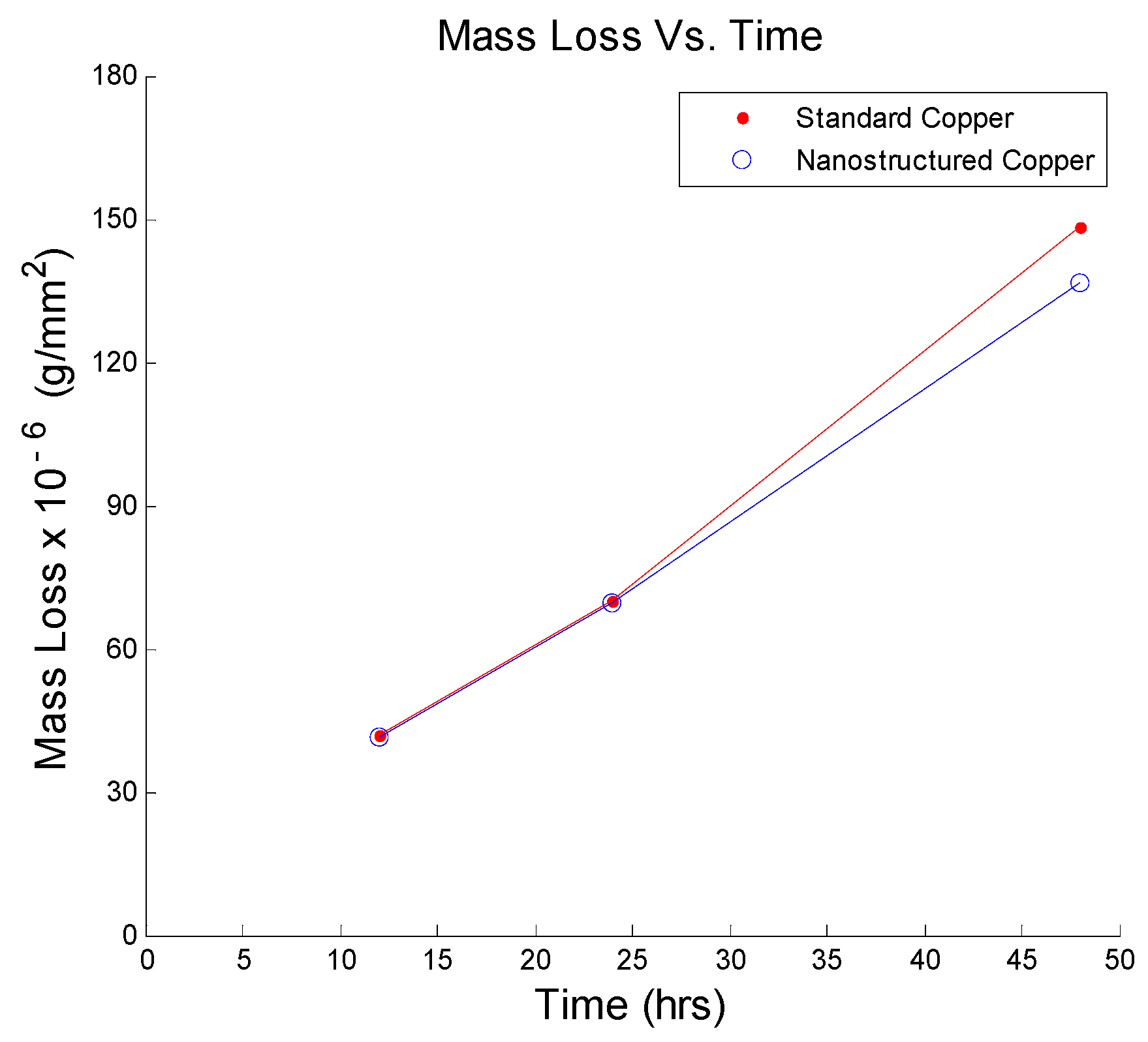
Figure 6.
Mass loss versus sand concentration for both standard and nanostructure copper.
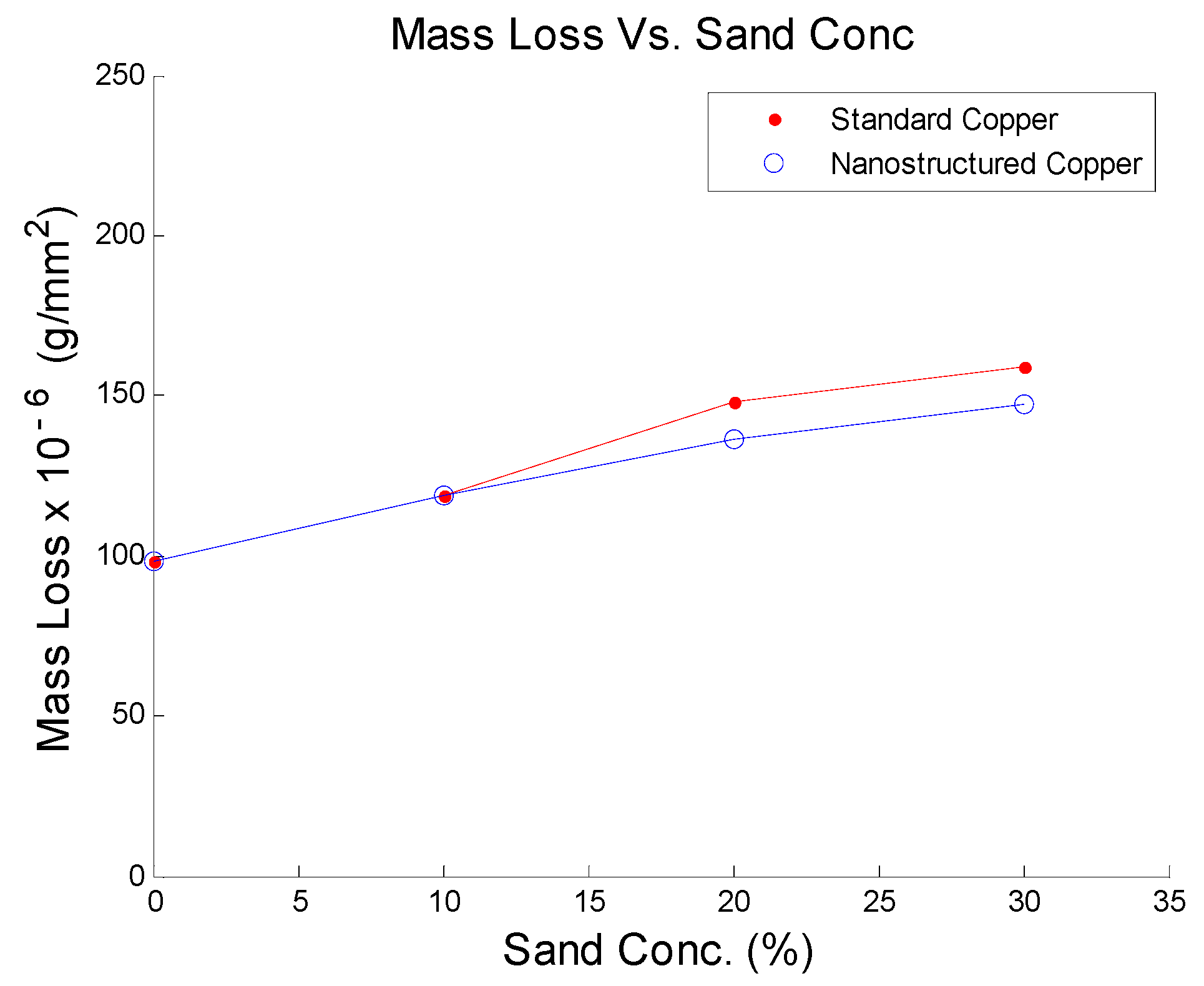
Figure 7.
Mass loss versus velocity and sand concentration for constant times (t = 20 h, 35 h, and 50 h); (a) First-order polynomial; (b) Second-order polynomial.
Figure 7.
Mass loss versus velocity and sand concentration for constant times (t = 20 h, 35 h, and 50 h); (a) First-order polynomial; (b) Second-order polynomial.
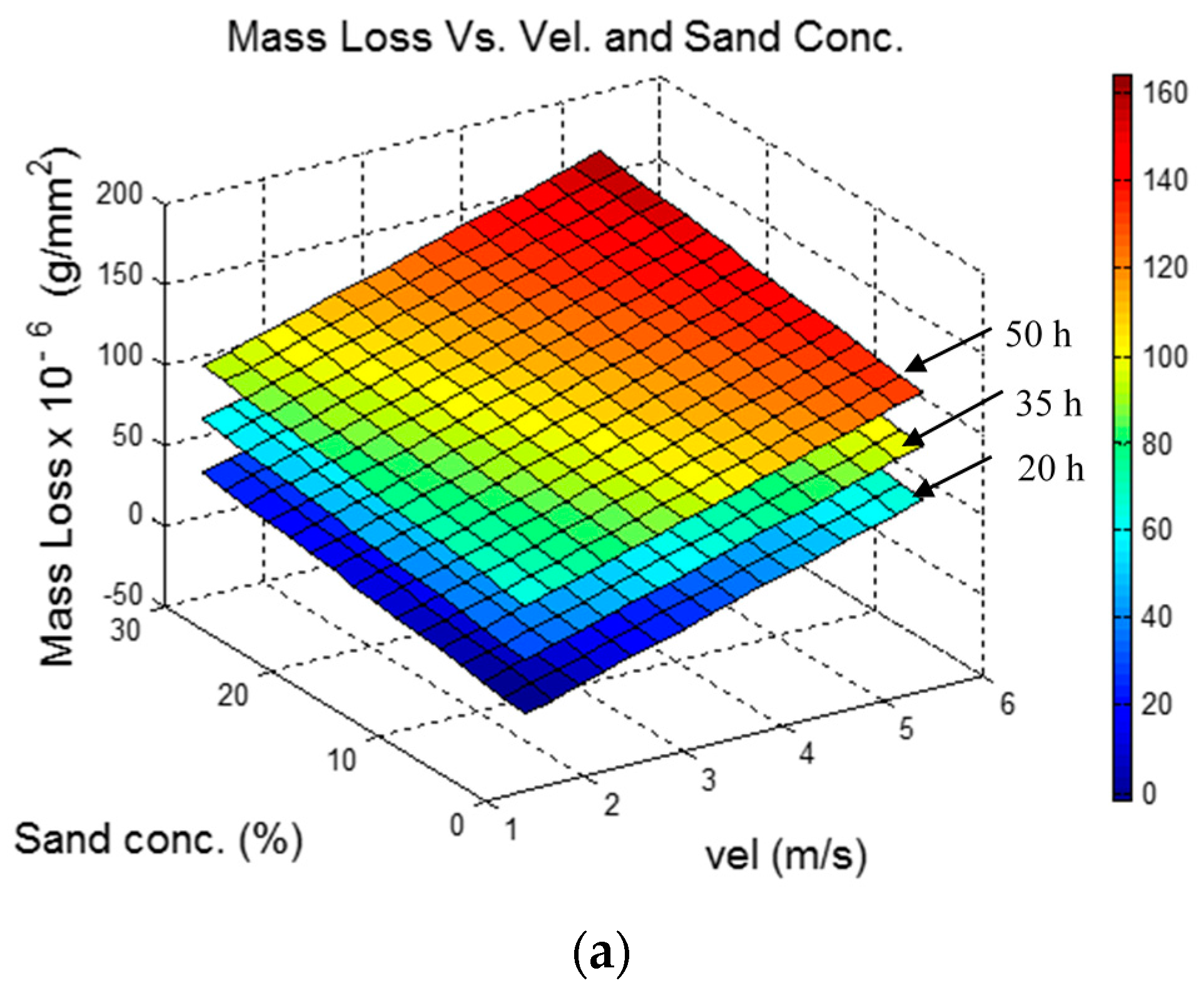

Figure 8.
Mass loss versus time and sand concentration for constant velocities (v = 2 m/s, 3.5 m/s, and 5 m/s); (a) First-order polynomial; (b) Second-order polynomial.
Figure 8.
Mass loss versus time and sand concentration for constant velocities (v = 2 m/s, 3.5 m/s, and 5 m/s); (a) First-order polynomial; (b) Second-order polynomial.

Figure 9.
Mass loss versus time and velocity for constant sand concentrations (s = 0%, 15%, and 30%); (a) First-order polynomial; (b) Second-order polynomial.
Figure 9.
Mass loss versus time and velocity for constant sand concentrations (s = 0%, 15%, and 30%); (a) First-order polynomial; (b) Second-order polynomial.
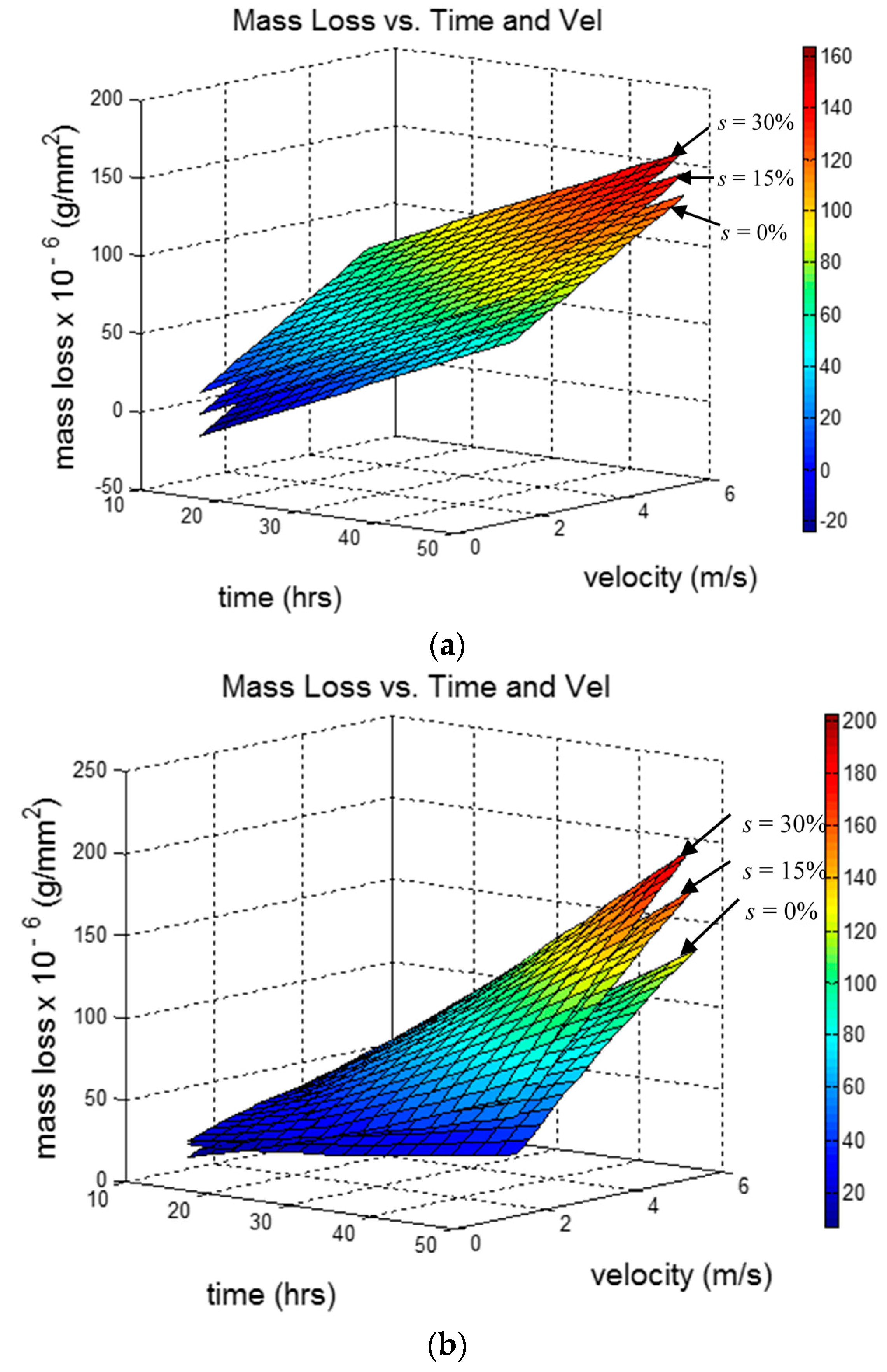
Figure 10.
Mass loss versus velocity and sand concentration for constant times (t = 20 h, 35 h, and 50 h); (a) First-order model; (b) Second-order model; (c) MSE for the first-order model; (d) MSE for the second-order model.
Figure 10.
Mass loss versus velocity and sand concentration for constant times (t = 20 h, 35 h, and 50 h); (a) First-order model; (b) Second-order model; (c) MSE for the first-order model; (d) MSE for the second-order model.


Figure 11.
Mass loss versus time and sand concentration for constant velocities (v = 2 m/s, 3.5 m/s, and 5 m/s); (a) First-order model; (b) Second-order model; (c) MSE for the first-order model; (d) MSE for the second-order model.
Figure 11.
Mass loss versus time and sand concentration for constant velocities (v = 2 m/s, 3.5 m/s, and 5 m/s); (a) First-order model; (b) Second-order model; (c) MSE for the first-order model; (d) MSE for the second-order model.

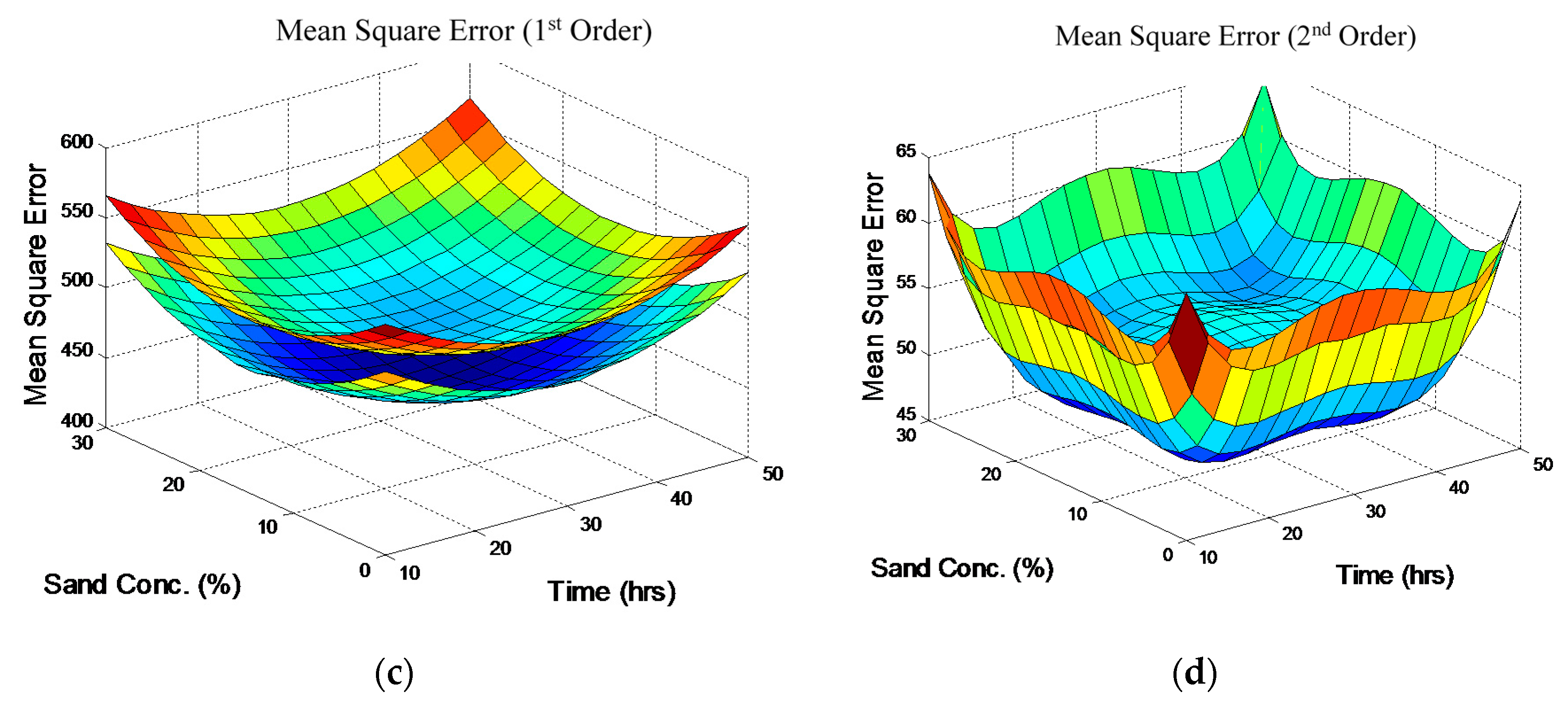
Figure 12.
Mass loss versus time and velocity for constant sand concentrations (s = 0%, 15%, and 30%); (a) First-order model; (b) Second-order model; (c) MSE for the first-order model; (d) MSE for the second-order model.
Figure 12.
Mass loss versus time and velocity for constant sand concentrations (s = 0%, 15%, and 30%); (a) First-order model; (b) Second-order model; (c) MSE for the first-order model; (d) MSE for the second-order model.


Table 1.
Chemical composition of the copper rods used in the study.
| Content | Cu | Fe | Pb | S | As | Sb | Bi |
|---|---|---|---|---|---|---|---|
| Composition (%) | 99.95 | 0.005 | 0.005 | 0.005 | 0.002 | 0.002 | 0.001 |
Table 2.
Lower and upper bounds for the test variables.
| Test Variables | Units | Lower Bound | Upper Bound |
|---|---|---|---|
| Test Time | hours | 10 | 50 |
| Impact Velocity | m/s | 1.4 | 5.4 |
| Sand Concentration | % | 0 | 30 |
Table 3.
Combinations of test points for the experiments.
| Test No. | Time (h) | Impact Velocity (m/s) | Sand Concentration % |
|---|---|---|---|
| 1 | 10 | 1.4 | 0 |
| 2 | 10 | 1.4 | 30 |
| 3 | 10 | 5.4 | 0 |
| 4 | 10 | 5.4 | 30 |
| 5 | 50 | 1.4 | 0 |
| 6 | 50 | 1.4 | 30 |
| 7 | 50 | 5.4 | 0 |
| 8 | 50 | 5.4 | 30 |
| 9 | 10 | 3.4 | 15 |
| 10 | 50 | 3.4 | 15 |
| 11 | 30 | 1.4 | 15 |
| 12 | 30 | 5.4 | 15 |
| 13 | 30 | 3.4 | 0 |
| 14 | 30 | 3.4 | 30 |
| 15 | 30 | 3.4 | 15 |
Table 4.
Test results from the E-C experiments.
| Test No. | Time (h) | Impact Velocity (m/s) | Sand Concentration (%) | Mass Loss Per Unit Area (μg/mm2) | ||
|---|---|---|---|---|---|---|
| Specimen 1 | Specimen 2 | Mean | ||||
| 1 | 10 | 1.4 | 0 | 7.6 | 10.2 | 8.9 |
| 2 | 10 | 1.4 | 30 | 11.3 | 12.8 | 12.1 |
| 3 | 10 | 5.4 | 0 | 29.2 | 31.5 | 30.4 |
| 4 | 10 | 5.4 | 30 | 42.3 | 49.8 | 46.1 |
| 5 | 50 | 1.4 | 0 | 38.0 | 32.9 | 35.4 |
| 6 | 50 | 1.4 | 30 | 60.8 | 70.2 | 65.5 |
| 7 | 50 | 5.4 | 0 | 130.6 | 134.7 | 132.6 |
| 8 | 50 | 5.4 | 30 | 210.3 | 204.7 | 207.5 |
| 9 | 10 | 3.4 | 15 | 26.8 | 30.3 | 28.6 |
| 10 | 50 | 3.4 | 15 | 136.7 | 126.1 | 131.4 |
| 11 | 30 | 1.4 | 15 | 43.3 | 45.4 | 44.3 |
| 12 | 30 | 5.4 | 15 | 102.9 | 97.2 | 100.0 |
| 13 | 30 | 3.4 | 0 | 62.9 | 61.5 | 62.2 |
| 14 | 30 | 3.4 | 30 | 74.7 | 83.5 | 79.1 |
| 15 | 30 | 3.4 | 15 | 64.5 | 67.0 | 65.8 |
Table 5.
Results from the regression.
| Polynomial Order | 1st Order | 2nd Order |
|---|---|---|
| Coefficient of Determination (r2) | 0.844 | 0.986 |
© 2017 by the authors. Licensee MDPI, Basel, Switzerland. This article is an open access article distributed under the terms and conditions of the Creative Commons Attribution (CC BY) license (http://creativecommons.org/licenses/by/4.0/).
Share and Cite
MDPI and ACS Style
Irfan, O.M.; Mukras, S.M.S.; Al-Mufadi, F.A.; Djavanroodi, F. Surface Modelling of Nanostructured Copper Subjected to Erosion-Corrosion. Metals 2017, 7, 155. https://doi.org/10.3390/met7050155
AMA Style
Irfan OM, Mukras SMS, Al-Mufadi FA, Djavanroodi F. Surface Modelling of Nanostructured Copper Subjected to Erosion-Corrosion. Metals. 2017; 7(5):155. https://doi.org/10.3390/met7050155
Chicago/Turabian StyleIrfan, Osama M., Saad M. S. Mukras, Fahad A. Al-Mufadi, and Faramarz Djavanroodi. 2017. "Surface Modelling of Nanostructured Copper Subjected to Erosion-Corrosion" Metals 7, no. 5: 155. https://doi.org/10.3390/met7050155
Note that from the first issue of 2016, this journal uses article numbers instead of page numbers. See further details here.