Determining Material Data for Welding Simulation of Presshardened Steel


1
Welding Engineering, Faculty of Mechanical Engineering, Chemnitz University of Technology, 09126 Chemnitz, Germany
2
Production Engineering, Faculty 6, Anhalt University of Applied Sciences, 06366 Koethen, Germany
*
Author to whom correspondence should be addressed.
Metals 2018, 8(10), 740; https://doi.org/10.3390/met8100740
Submission received: 4 September 2018
/
Revised: 17 September 2018
/
Accepted: 18 September 2018
/
Published: 20 September 2018
(This article belongs to the Special Issue Science, Characterization and Technology of Joining and Welding)
Abstract
:In automotive body-in-white production, presshardened 22MnB5 steel is the most widely used ultra-high-strength steel grade. Welding is the most important faying technique for this steel type, as other faying technologies often cannot deliver the same strength-to-cost ratio. In order to conduct precise numerical simulations of the welding process, flow stress curves and thermophysical properties from room temperature up to the melting point are required. Sheet metal parts made out of 22MnB5 are welded in a presshardened, that is, martensitic state. On the contrary, only flow stress curves for soft annealed or austenitized 22MnB5 are available in the literature. Available physical material data does not cover the required temperature range or is not available at all. This work provides experimentally determined hot-flow stress curves for rapid heating of 22MnB5 from the martensitic state. The data is complemented by a comprehensive set of thermophysical data of 22MnB5 between room temperature and melting. Materials simulation methods as well as a critical literature review were employed to obtain sound thermophysical data. A comparison of the numerically computed nugget growth curve in spot welding with experimental welding results ensures the validity of the hot-flow stress curves and thermophysical data presented.
1. Introduction
The finite-element analysis (FEA) of welding processes like spot and arc welding has a key role in the design of the faying process. The part design can be significantly influenced or even determined by requirements of the welding technology. Weldment properties eventually will determine the mechanical performance of the welded structure. Tolerances in industrial production are critical influences on the choice of welding processes and parameters, as pointed out by Podržaj et al. [1] as well as Schlosser and Jüttner [2] and Häßler and Füssel [3]. While Brauser et al. [4] emphasized the effect of gaps on spot welding quality, Moos and Vezzetti [5] for the first time employed FEA to further investigate the effect of tolerances in complex assemblies. Bi et al. [6] employed FEA to examine shunting at a challenging three-sheet joint, whereas van der Aa et al. [7] optimized the welding parameters of a new automotive steel grade using FEA. In the course of product development, FEA can therefore greatly reduce the probability of faulty designs and the necessity to carry out preliminary tests. This helps to save design costs and time, releasing resources to develop better-performing, more-lightweight welded structures.
The numerical simulation of welding processes and welding results is a challenging task. Reasons are the strong multiphysical couplings of phenomena and the steep temperature gradients at the weld site. With increasing material temperature, significant nonlinear changes in the material properties occur. As a result, a spatial field of local material properties, with steep gradients, will be present around the weld site, affecting the physics and the result of the welding process, and in turn, the numerical solution process. This necessitates a very careful selection of FEA boundary conditions, as shown by Raoelison et al. [8], and material data suitable for the specific temperature profiles of welding, as Schwenk and Rethmeier [9] emphasized. In order to carry out precise numerical simulations of the welding process, a complete dataset of physical and mechanical material properties up to the melting point is essential. According to Schwenk and Rethmeier [9], the dataset needs to include as a function of temperature:
- flow stress ;
- elastic modulus E and Poisson ratio ;
- coefficient of thermal expansion ;
- specific electrical resistance ;
- mass density ;
- specific heat capacity /specific entropy ; and
- specific thermal conductivity .
As explained by Karbasian and Tekkaya [10], automotive parts made of 22MnB5 are heat-treated before the welding process. During the heat treatment, the desired, sometimes localised, martensitic microstructure with high strength is established. Merklein et al. [11] reported on various works on the production of load-adjusted parts with locally tailored properties by means of a tailored heat treatment. In the as-delivered state, 22MnB5 has a ferritic–pearlitic microstructure as Geiger et al. [12] stated. This peculiarity of 22MnB5 has important consequences. The flow stress curves available in the literature, as provided by Ngyuen et al. [13], are intended to be used for hot-stamping simulations of the material. This means that in mechanical testing, the material is fully austenitized before it is cooled down to the respective test temperature; cf. Merklein and Lechler [14] as well as Naderi [15]. In contrary to that, in the welding process the material is being heated up from the martensitic state to the respective temperature very quickly. As reported by Gumbsch et al. [16], significant softening of the material will occur although the temperature is not surpassed, that is, the martensite is only tempered. Consequently, the flow stress curves available are not valid for the welding simulation. Few authors have published information on the temperature-dependent physical properties of 22MnB5: Shapiro [17]; Spittel and Spittel [18]; and Wink and Kraetschmer [19]. In those datasets, various properties are missing altogether, while others are only available for a temperature range not sufficient for the welding process simulation.
It is the goal of this work to supplement the datasets available for 22MnB5 in the martensitic state by means of measurements, numerical computation and literature review. Although the scope of this work lies in the data application in spot welding, the data can be used for other welding processes as well.
2. Materials and Methods
2.1. Experimental
2.1.1. Test Procedure
Flow stress curves of 22MnB5 were measured using a DIL805 A/D Dilatometer built by Baehr (Thermoanalyse GmbH, Huellhorst, Germany), shown in Figure 1. The specimens depicted in Figure 2 were cut out of the as-delivered sheet of 22MnB5 with 1.5 mm thickness by a water jet, and afterwards the coating was ground off. In the dilatometer, each specimen was induction-heated under vacuum to 1223 K within 180 s and soaked for 120 s. Following a Newtonian cooling law, the specimens were then quenched to 343 K with an average cooling rate of using argon gas. This temperature was held for another 120 s to allow some relief of residual stresses. Additional microsections and tensile tests proved that this initial heating and cooling cycle appropriately yields the desired martensitic microstructure in the specimens, and in turn resembles the presshardening process mentioned in the previous section.
Afterwards, the specimens were heated up with to the test temperature , followed by a soaking time of 2 s. While force and elongation were measured, the sample was then elongated with a (Hencky) strain rate of . A welded-on thermocouple of the type Pt/Pt10Rh ensured correct temperature control throughout the test. The specimen was neither intentionally strained to fracture, nor was the elongation at rupture evaluated. For test temperatures up to and including , three specimens per temperature were tested; at higher temperatures, the low scatter of the data allowed a reduction to two specimens. Due to the high strength of 22MnB5, dilatometric tests at temperatures lower than were not possible within the machine’s limitations. Additional tests on a conventional tensile testing machine at room temperature therefore supplemented the experiments. The highest temperature tested was .
2.1.2. Data Processing
Each measured force–elongation curve was transformed into a stress–strain curve and limited to strain values up to uniform elongation. A regression analysis then determined the parameters of the flow stress Equation (1) by Hockett and Sherby [20] to best fulfil the individual measured curve.
Therein, is the initial flow stress and the saturation flow stress. and are dimensionless parameters. The resulting flow stress is valid for a respective temperature . The mean of the computed Hockett–Sherby parameters within an individual test temperature then yielded the parameters of the mean flow stress curve for the respective temperature. The molten metal at the weld is described using the same structural mechanics equations as the solid material, instead of defining a multiphase approach using the Navier–Stokes equation for the molten metal. This simplification significantly eases modelling and computation of the welding process. As melt flow in most cases is little, it is allowed. Of course, molten metal will have no yield strength nonetheless. Therefore, it is formally necessary to also define flow stress curves for the melt. A virtual zero-strength, as defined below, and a finite compressibility, cf. Section 3.2.1, in this case were determined as the most reasonable material properties of the melt. In spot welding simulations by the authors, see Section 3.3 and [21], good results have been achieved by defining two additional curves fulfilling
In short, regions governed by laws of fluid flow in the FEA are represented by means of drastically reduced flow stress.
Input of the data into the FEA was required in the form of stress–Cauchy–strain curves. The strain values therein were transformed from the Hencky–strain applying the relation
2.2. Numerical Material Simulation
Measurement of physical properties at elevated temperatures during rapid heating is very difficult, as shown by [22,23], which inform on the comparably large measurement errors that have to be expected. Material simulation software like Jmatpro can deliver the required data, but the reliability of the results is questionable, as the software purely relies on empirical models. Therefore, the decision was made to compute the required data using the software, and then validate the data very critically in comparison to measured data available in the literature.
Using the software, the phase composition, as well as the physical properties of the pure phases during heating of the material, were computed. Afterwards, the physical properties of the temperature-dependent phase composition were computed from the properties of the pure phases by using the lever rule. The computed austenitization temperatures for a heating rate of are presented in Table 1. It can be seen that the transformation delay due to the heating rate is small compared to the temperatures stated by [24].
The tempering, as well as partial or full dissolving of martensite below , is driven by diffusional processes. During quick heating of the material, the dwell time below is short. Therefore, diffusive effects are negligible. In this work, it was accordingly assumed that between and the martensite will directly transform into austenite. Figure 3 depicts the phase composition of 22MnB5 being assumed in the thermophysical material property computation with Jmatpro.
It has to be pointed out that the assumption of neglected tempering in this work was only done for considerations regarding the thermophysical properties of 22MnB5. The flow stress curves on the contrary are derived from measurements, hence including the tempering effect of martensite as well.
The data computed with Jmatpro was compared to data published by: Bungardt and Spyra (BaS) [25], Spittel and Spittel [18] (Landoldt-Boernstein), Richter [26,27], Shapiro [17], Verein Deutscher Eisenhuettenleute (VDEh) [23], Volz [28] and Wink and Kraetschmer [19]. From a chemical composition point of view, 22MnB5 is an unalloyed steel. Therefore, it is allowed to compare the order of magnitude of the computed data to data of similar unalloyed steels and pure iron, at least for the austenitic and molten phases. Accordingly, literature data on pure iron and a 23Mn6 steel were included in the comparison to ensure best verification of the data derived from Jmatpro. The data published by Volz [28] was collected from additional literature sources and is valid for structural steel. He used the data for FEAs of residual stresses resulting from arc welding and obtained very good conformity to his experimental verifications. Therefore, the data is considered to be sound.
During melting of the material, some properties considerably change their magnitude. Simulation trial runs proved that the numerical solution procedure is significantly more stable when the melting range of the material is only slightly widened. To account for this effect, the temperatures and were artificially shifted about upwards and downwards, respectively; cf. the data points ‘FEA’ in the diagrams outlined below. An effect of this temperature shift on the computed results was not observed.
During solution of the model, the equation solver may compute very large, intermediate temperature results. In order to enhance the numerical stability, the physical data was extrapolated up to the boiling point accordingly.
2.3. Resistance Spot Welding Simulation and Welding Experiments
The material data presented is well proven by comparing the results of a spot welding process FEA to measured results. A two-staged welding current as presented in Figure 4 along with a constant electrode force of was applied in both experiment and FEA. The experiments were carried out with a pneumatic spot welding gun with high-frequency direct current (HFDC) power source. With respect to the scope of this work, details on the experimental conditions, FE model and the entirety of its boundary conditions shall be examined in [29].
3. Results and Discussion
It has to be noted that the data presented is valid only for the heating phase in the welding process, as it is intended to be used in simulation-driven process development. Material property evolution in the cooling phase is not within the scope of this work. The data represented by the points denoted as ‘FEA’ in the diagrams is tabularly composed in Section 3.4.
3.1. Flow Stress
Figure 5 displays the measured flow stress curves, along with the two artificial curves. The curves have been extended according to (1) up to . It can be readily seen that the work hardening effect is not pronounced in the martensitic phase. As soon as is surpassed, significant strain hardening becomes visible. It shall be noted that the ends of the curves do not indicate fracture of the material. At most temperatures it will fail much earlier. Due to experimental limitations outlined above, a significant gap in the data exists between and . As the decrease of strength in this temperature window is moderate, it is assumed that a linear interpolation between the respective curves, as FEA software modules will perform it, is reasonable.
3.2. Physical Properties
3.2.1. Elastic Modulus and Poisson Ratio
Starting from , the elastic modulus decreases with temperature, while the Poisson ratio increases, as shown in Figure 6. For the melt, the software computed a very small elastic modulus along with incompressible material behaviour (), but delivered a small, finite bulk modulus . In other words, the computed bulk modulus and Poisson ratio excluded each other. Due to lack of other data, the computed bulk modulus was then used to compute the elastic modulus of the melt using the relation:
As fully incompressible behaviour is unlikely for the melt, the Poisson ratio therein was set to . This prevents numerical problems resulting from incompressible material behaviour, but still reasonably represents the data computed by Jmatpro.
3.2.2. Coefficient of Thermal Expansion
The data depicted in Figure 7 represents the secant coefficient of thermal expansion with a reference temperature of . Some of the literature data therein has been computed from the lattice constant taken from [23]. The coefficient of thermal expansion strongly depends on the lattice structure, as shown in Figure 7. During austenitization, it quickly drops, followed by a steeper incline. On melting, the coefficient roughly doubles its magnitude.
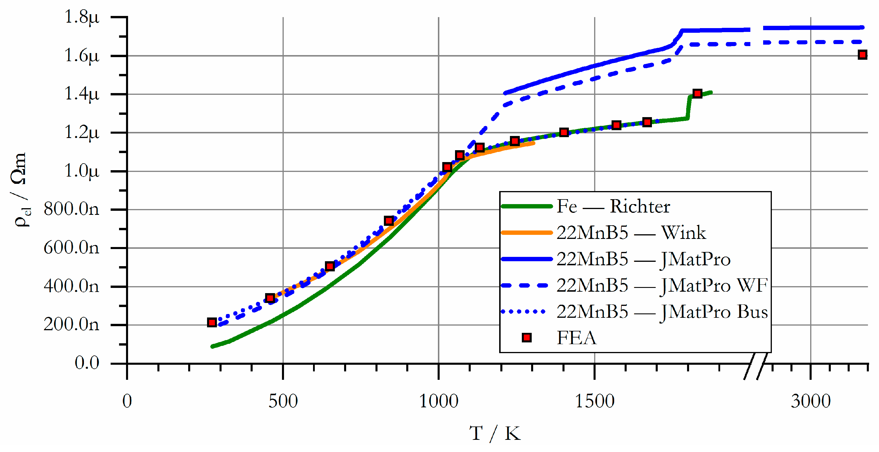
3.2.3. Specific Electric Resistance
To improve readability, the specific electric resistance is drawn in two separate diagrams, shown in Figure 8 and Figure 9. Literature data on this property is particularly scarce. Jmatpro delivered data on the specific resistance only for . To fill the gap, additional data was generated based on the thermal conductivity using the Wiedemann–Franz (WF) law with a Lorenz number of as stated by [30]:
as well as the relation published by BaS [25],
Close to room temperature, the specific resistance is strongly dependent on the alloy. With increasing temperature, the curves converge towards each other. At the melting point, the resistance increases by a small percentage. For the austenite and the melt, the data delivered by Jmatpro and the WF law are in contradiction with the experimental data. The data computed with the model of BaS is in good conformity with the experimental data. Accordingly, the data computed with the BaS rule is considered to be sound. Beyond the melting point, the curve was extrapolated up to the boiling point.
3.2.4. Mass Density
In addition to the thermal expansion of the metal during heating, its mass density generally decreases, as shown in Figure 10. On austenitization, the density increases by a small percentage accordingly. It is critical that the data on thermal expansion and density fit to each other. Otherwise, creation or destruction of mass in the numerical model, with adverse effects for the precision of the thermal balance, would occur. The mass density data presented here has been carefully reviewed regarding this subject, although mathematical details on the review shall not be discussed.
3.2.5. Specific Heat Capacity
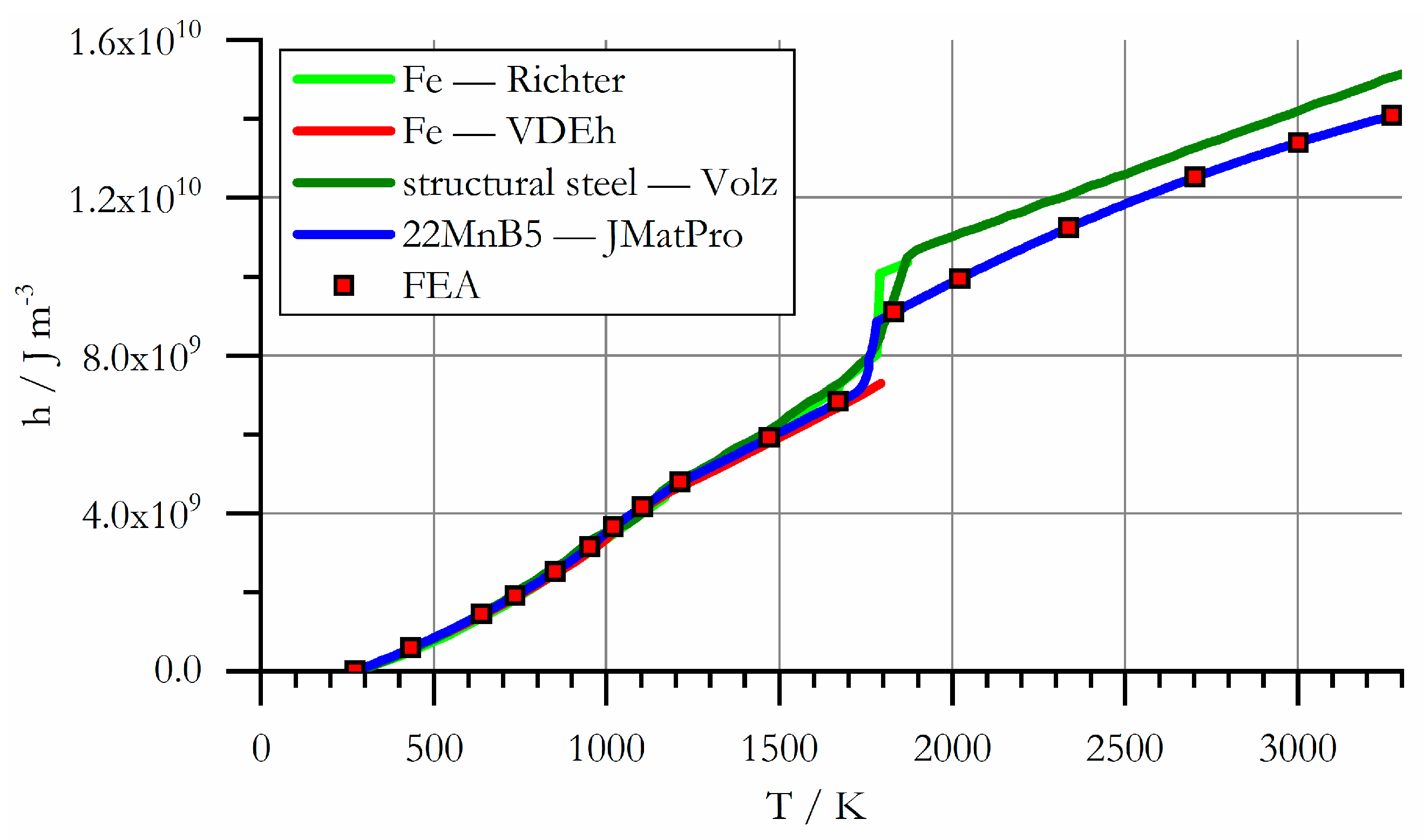
The specific heat capacity is a function of temperature with discontinuities at the Curie point, during austenitization, and at the melting point, as shown in Figure 11. At the mentioned transition points, the heat capacity is theoretically infinite. To avoid the discontinuities, the specific enthalpy density is used by the FEA following the relation
The integrated heat capacity curves according to the relation are presented in Figure 12. Therein, an average mass density of was set. While the average slope of the curve is relatively constant, melting is characterised by a significant step in the curve.
3.2.6. Specific Thermal Conductivity
The specific thermal conductivity is initially reduced with increasing temperature, but increases again as soon as austenitization sets in, as shown in Figure 13. The data computed by Jmatpro is in good agreement with the experimental data. The curve published by Shapiro [17] apparently refers to the cooling of the material from the austenitic state. An additional curve computed by Jmatpro for quenching of 22MnB5 being drawn in Figure 13 strongly supports this. As computed by [31,32], a hydrodynamic mixing movement will occur in the molten pool during welding. In order to account for the resulting additional convective heat transport, the specific thermal conductivity of the melt is increased by about twice the magnitude at room temperature in this analysis.
3.3. Data Application in Resistance Spot Welding
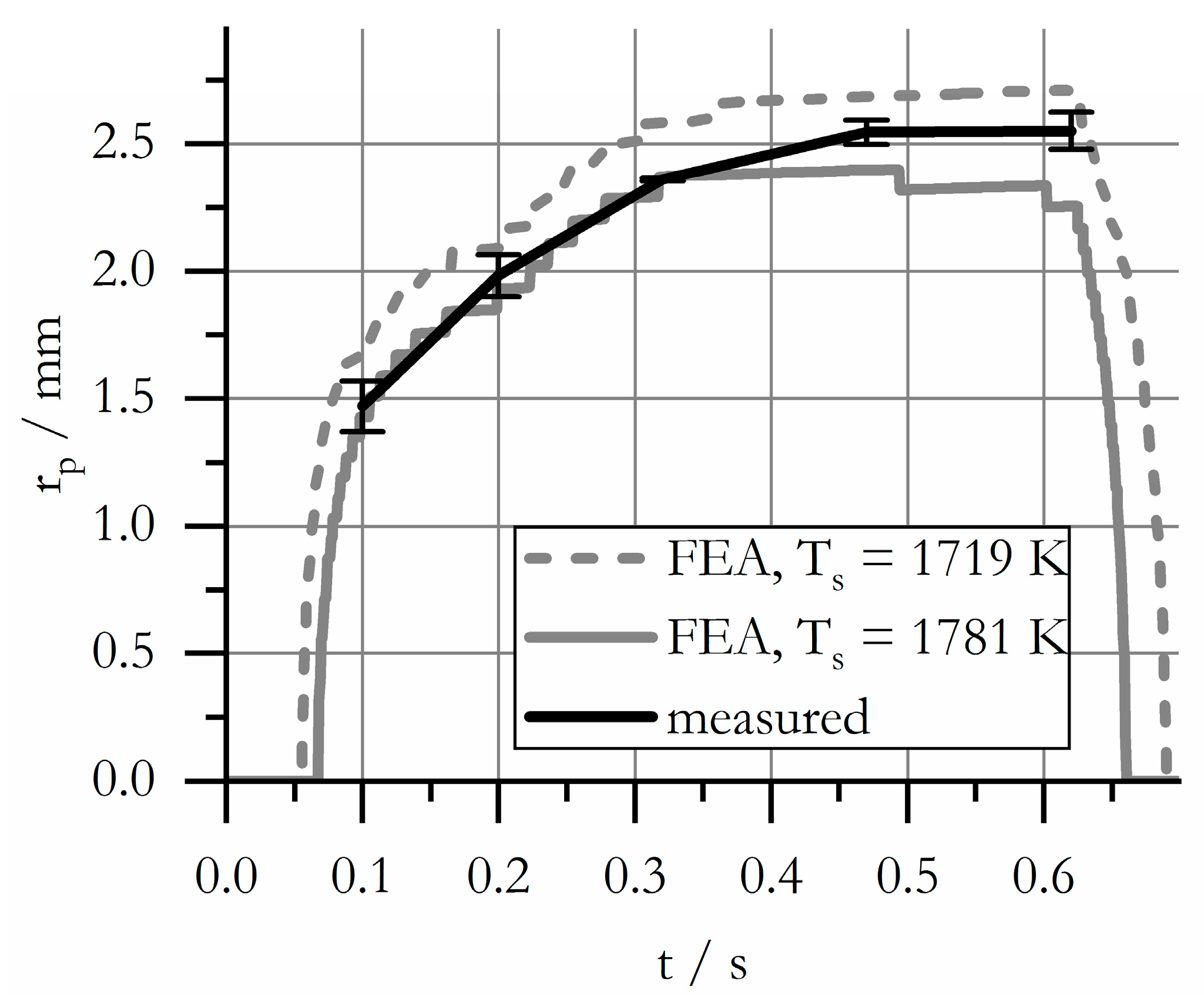
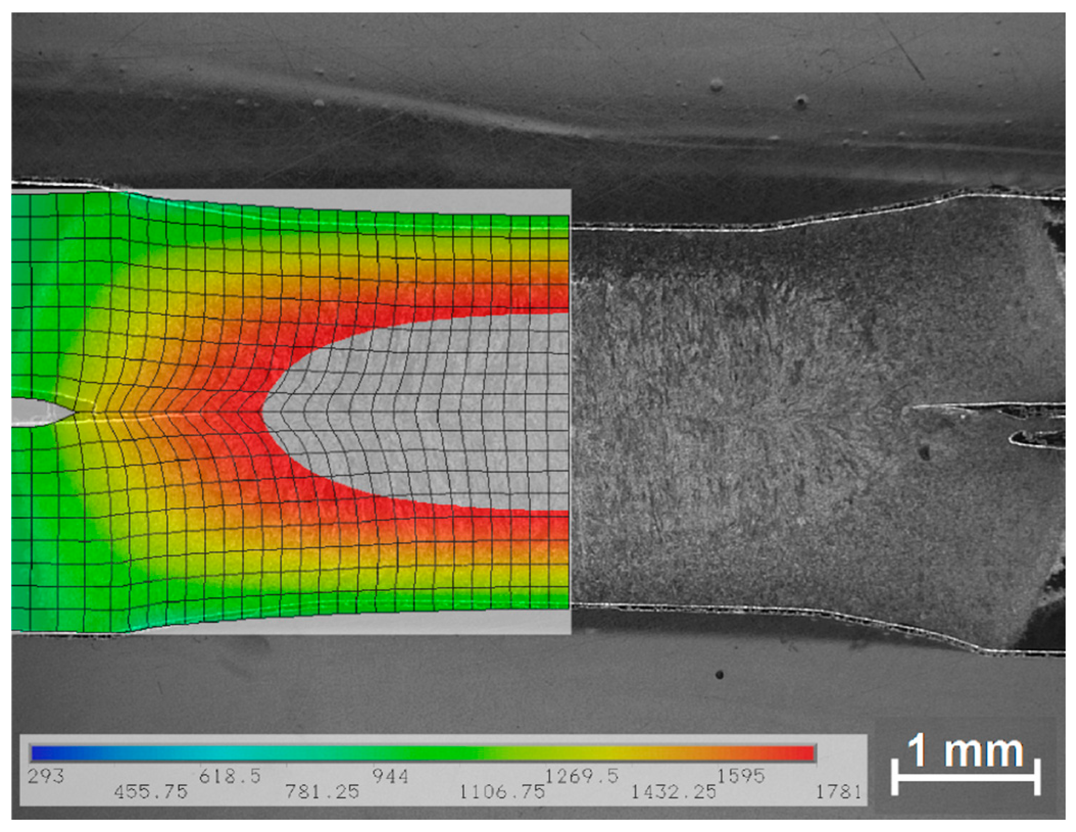
An overview of the computed temperature distribution in the welded sheets at the end of current flow, along with a macrosection of the weld nugget, is presented in Figure 14.
The computed molten zone represents the nugget shape visible in the macrosection reasonably well, although the computed nugget is slightly smaller. Quantitative examination of the nugget radius in Figure 15 gives more insight: In the FEA, a decision has to be made whether the temperature A4 or AS is considered to be sufficient to form a joint across the sheet metals’ surfaces. The experimentally observed nugget growth curve lies well in between both criteria. In Figure 14, melting is only assumed when the temperature AS is surpassed, which explains the seemingly too-small nugget in the picture. It shall also be noted that the computed electrode indentation depth and shape conform very well with the experiment. By comparison of the sheet thicknesses on the left border of Figure 14, it is assured that the relative scaling of FEA and the macrosection is correct.
3.4. Tabular Data
4. Conclusions
Measurements of flow stress curves, as well as physical material property computations and comprehensive literature reviews, were employed to compose a set of material data necessary for welding process simulations on presshardened 22MnB5 steel. Due to the lack of literature data and/or specific requirements, a few simplifications and assumptions were made in the process of the data collection. The assumptions are described in detail in this work, so the simulation expert may carefully reconsider if the data is still valid in the specific case. The data provided is suitable to describe the materials’ behaviour during the heating phase in the welding process. The materials’ behaviour during cooling or quenching is not in the scope of this work.
The following results were obtained:
- Data on the flow stress of 22MnB5 was measured and converted to stress–strain data for test temperatures ranging from to .
- Flow stress data is provided by means of flow parameters for the tested temperatures according to the Hockett–Sherby model.
- Physical material property data of 22MnB5 as a function of temperature has been computed using material simulation software. The data was critically reviewed considering literature data.
All datasets provided have been linearly extrapolated up to a temperature of in order to allow immediate use for the numerical process simulation procedure.
Author Contributions
Conceptualization, J.K.; Data curation, J.K., P.M. and K.K.; Formal analysis, J.K. and K.K.; Investigation, J.K.; Methodology, J.K.; Project administration, J.K.; Resources, P.M.; Software, P.M.; Supervision, P.M. and K.K.; Validation, J.K. and K.K.; Visualization, J.K.; Writing–review & editing, J.K. and P.M.
Funding
The publication costs of this article were funded by the German Research Foundation/DFG and Chemnitz University in the funding programme Open Access Publishing.
Conflicts of Interest
The authors declare no conflict of interest.
References
- Podržaj, P.; Jerman, B.; Simončič, S. Poor fit-up condition in resistance spot welding. J. Mater. Process. Technol. 2016, 230, 21–25. [Google Scholar] [CrossRef]
- Schlosser, B.; Jüttner, S. Indikatoren zur Beurteilung der Qualität von MSG-Schweißnähten. In 35. Assistentenseminar Füge- und Schweißtechnik; DVS Media: Magdeburg, Germany, 2016; Volume 314. [Google Scholar]
- Häßler, M.; Füssel, U. Fügen hochbeanspruchter Stähle durch kathodenfokussiertes WIG-Löten (CF-TIG). In 35. Assistentenseminar Füge- und Schweißtechnik; DVS Media: Magdeburg, Germany, 2016; Volume 314. [Google Scholar]
- Brauser, S.; Pepke, L.-A.; Weber, G.; Rethmeier, M. Influence of Production-Related Gaps on Strength Properties and Deformation Behaviour of Spot Welded Trip Steel HCT690T. Weld. World 2012, 56, 115–125. [Google Scholar] [CrossRef]
- Moos, S.; Vezzetti, E. Compliant assembly tolerance analysis: Guidelines to formalize the resistance spot welding plasticity effects. Int. J. Adv. Manuf. Technol. 2012, 61, 503–518. [Google Scholar] [CrossRef]
- Bi, J.; Song, J.; Wei, Q.; Zhang, Y.; Li, Y.; Luo, Z. Characteristics of shunting in resistance spot welding for dissimilar unequal-thickness aluminum alloys under large thickness ratio. Mater. Des. 2016, 101, 226–235. [Google Scholar] [CrossRef]
- Van der Aa, E.; Amirthalingam, M.; Winter, J.; Hanlon, D.N.; Hermans, M.J.M.; Rijnders, M.; Richardson, I.M. Improved Resistance Spot Weldability of 3rd Generation AHHS for Automotive Applications. Math. Model. Weld Phenoma 2016, 11, 175–193. [Google Scholar]
- Raoelison, R.N.; Fuentes, A.; Pouvreau, C.; Rogeon, P.; Carré, P.; Dechalotte, F. Modeling and numerical simulation of the resistance spot welding of zinc coated steel sheets using rounded tip electrode: Analysis of required conditions. Appl. Math. Model. 2014, 38, 2505–2521. [Google Scholar] [CrossRef]
- Schwenk, C.; Rethmeier, M. Material Properties for Welding Simulation—Measurement, Analysis and Exemplary Data. Weld. J. 2011, 90, 220–227. [Google Scholar]
- Karbasian, H.; Tekkaya, A.E. A review on hot stamping. J. Mater. Process. Technol. 2010, 210, 2103–2118. [Google Scholar] [CrossRef]
- Merklein, M.; Johannes, M.; Lechner, M.; Kuppert, A. A review on tailored blanks—Production, applications and evaluation. J. Mater. Process. Technol. 2014, 214, 151–164. [Google Scholar] [CrossRef]
- Geiger, M.; Merklein, M.; Hoff, C. Basic Investigations on the Hot Stamping Steel 22MnB5. Adv. Mater. Res. 2005, 6–8, 795–804. [Google Scholar] [CrossRef]
- Ngyuen, D.-T.; Banh, T.-L.; Jung, D.-W.; Yang, S.-H.; Kim, Y.-S. A Modified Johnson-Cook Model to Predict Stress-Strain Curves of Boron Steel Sheets at Elevated and Cooling Temperatures. High Temp. Mater. Proc. 2012, 31, 37–45. [Google Scholar]
- Merklein, M.; Lechler, J. Investigation of the thermo-mechanical properties of hot stamping steels. J. Mater. Process. Technol. 2006, 177, 452–455. [Google Scholar] [CrossRef]
- Naderi, M. A Numerical and Experimental Investigation into Hot Stamping of Boron Alloyed Heat Treated Steels. Steel Res. Int. 2008, 79, 77–84. [Google Scholar] [CrossRef]
- Gumbsch, P.; Roos, E.; Hahn, O. Charakterisierung und Ersatzmodellierung des Bruchverhaltens von Punktschweißverbindungen an ultrahochfesten Stählen für die Crashsimulation unter Berücksichtigung der Auswirkung der Verbindung auf das Bauteilverhalten; Fraunhofer Institut IWM: Freiburg, Germany; MPA Stuttgart: Stuttgart, Germany; Universität Paderborn: Paderborn, Germany, 2012. [Google Scholar]
- Shapiro, A. Finite Element Modeling of Hot Stamping. Steel Res. Int. 2009, 80, 658–664. [Google Scholar] [CrossRef]
- Spittel, M.; Spittel, T. Steel symbol/number: 22MnB5/1.5528. In Metal Forming Data of Ferrous Alloys—Deformation Behaviour; Warlimont, H., Ed.; Landolt-Börnstein—Group VIII Advanced Materials and Technologies; Springer: Berlin/Heidelberg, Germany, 2009; Volume 2C1. [Google Scholar]
- Wink, H.-J.; Krätschmer, D. Charakterisierung und Modellierung des Bruchverhaltens von Punktschweißverbindungen in pressgehärteten Stählen—Simulation des Schweißprozesses. In Proceedings of the 11. LS-DYNA Forum, Ulm, Germany, 9–10 October 2012. [Google Scholar]
- Hockett, J.E.; Sherby, O.D. Large strain deformation of polycrystalline metals at low homologous temperatures. J. Mech. Phys. Solids 1975, 23, 87–98. [Google Scholar] [CrossRef]
- Kaars, J.; Mayr, P.; Koppe, K. Simple Transition Resistance Model for Spot Welding Simulation of aluminized AHSS. Math. Model. Weld Phenoma 2016, 11, 685–702. [Google Scholar]
- Byl, C.; Bérardan, D.; Dragoe, N. Experimental setup for measurements of transport properties at high temperature and under controlled atmosphere. Meas. Sci. Technol. 2012, 23, 035603. [Google Scholar] [CrossRef]
- Werkstoffkunde Stahl; Eisenhüttenleute, V.D. (Ed.) Springer: Berlin/Heidelberg, Germany, 1984. [Google Scholar]
- Naderi, M.; Saeed-Akbari, A.; Bleck, W. The effects of non-isothermal deformation on martensitic transformation in 22MnB5 steel. Mater. Sci. Eng. A 2008, 487, 445–455. [Google Scholar] [CrossRef]
- Bungardt, K.; Spyra, W. Wärmeleitfähigkeit von Stählen und Legierungen bei Temperaturen Zwischen 20 °C und 700 °C; Verlag Stahleisen: Düsseldorf, Germany, 1965. [Google Scholar]
- Richter, F. Die wichtigsten physikalischen Eigenschaften von 52 Stahlwerkstoffen. Stahleisen Sonderberichte 1973, 8, 1–32. [Google Scholar]
- Richter, F. Physikalische Eigenschaften von Stählen und ihre Temperaturabhängigkeit. In Stahleisen Sonderberichte; Verlag Stahleisen: Düsseldorf, Germany, 1983. [Google Scholar]
- Volz, M. Die Rissentstehung in Statisch Beanspruchten Stahlkonstruktionen unter Berücksichtigung von Schweißeigenspannungen. Ph.D. Thesis, Universität Karlsruhe (TH), Karlsruhe, Germany, 2009. [Google Scholar]
- Kaars, J.; Mayr, P.; Koppe, K. Generalized dynamic transition resistance in spot welding of aluminized 22MnB5. Mater. Des. 2016, 106, 139–145. [Google Scholar] [CrossRef]
- Thermal Conductivity of Pure Metals and Alloys; Madelung, O.; White, G.K. (Eds.) Landolt-Börnstein—Group III Condensed Matter; Springer: Berlin/Heidelberg, Germany, 1991; Volume 15c. [Google Scholar]
- Li, Y.B.; Lin, Z.Q.; Lai, X.M.; Chen, G.L. Electromagnetic Phenomena in Resistance Spot Welding and its Effects on Weld Nugget Formation. In Proceedings of the PIERS Proceedings, Moscow, Russia, 18–21 August 2009. [Google Scholar]
- Na, S.J.; Cheon, J.H.; Kiran, D.V.; Cho, D.W. Heat and Mass Flow in Arc Welding Processes and its Application to Mechanical Analysis of Welded Structures. Math. Model. Weld Phenoma 2016, 11, 5–22. [Google Scholar]
Figure 1.
Austenitization of a specimen in the dilatometer.
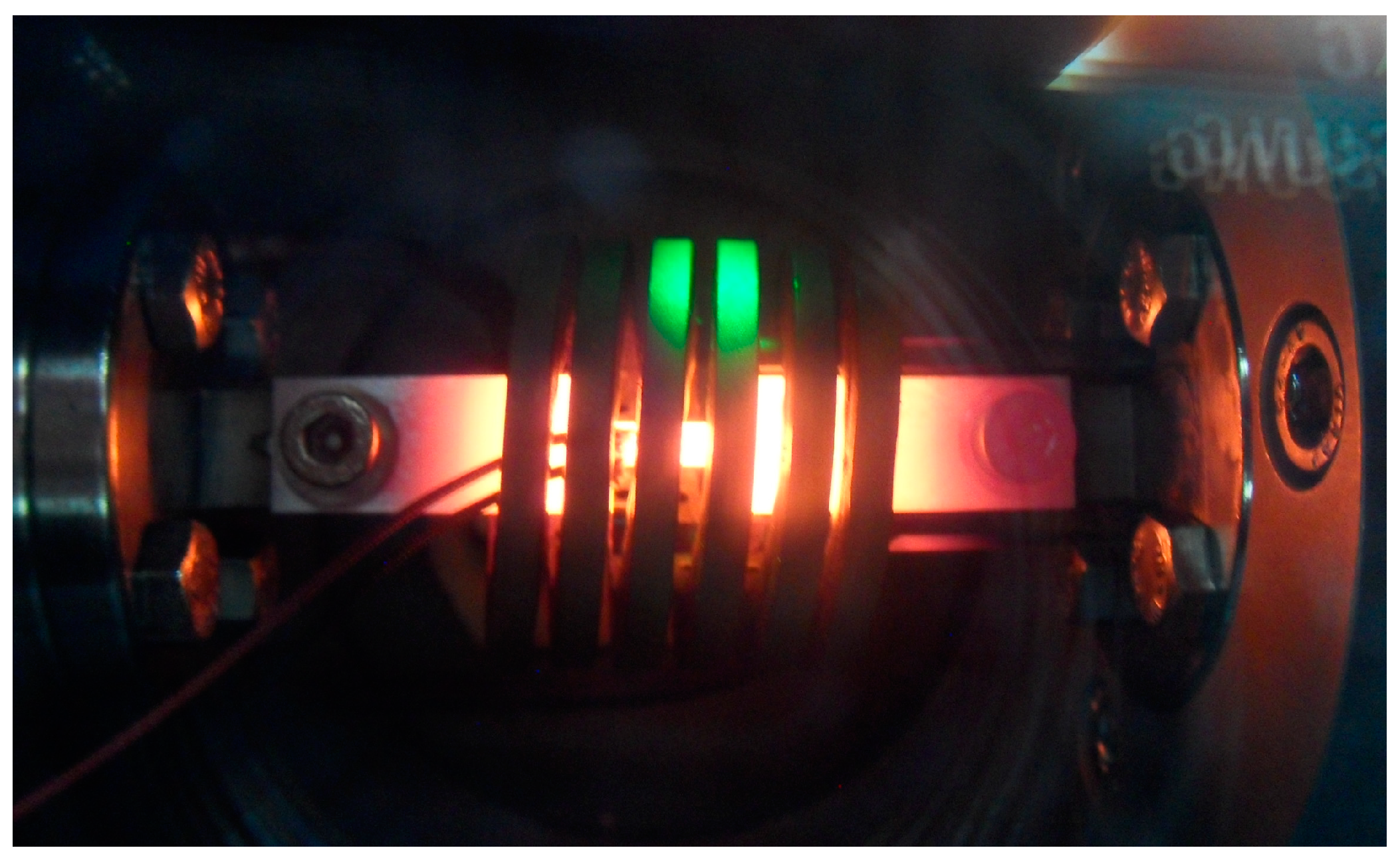
Figure 2.
Some specimens after the hot tensile test in the dilatometer.
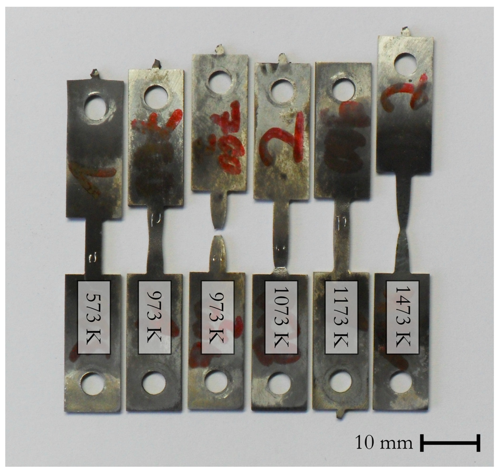
Figure 3.
Phase fractions of 22MnB5 during heating with .
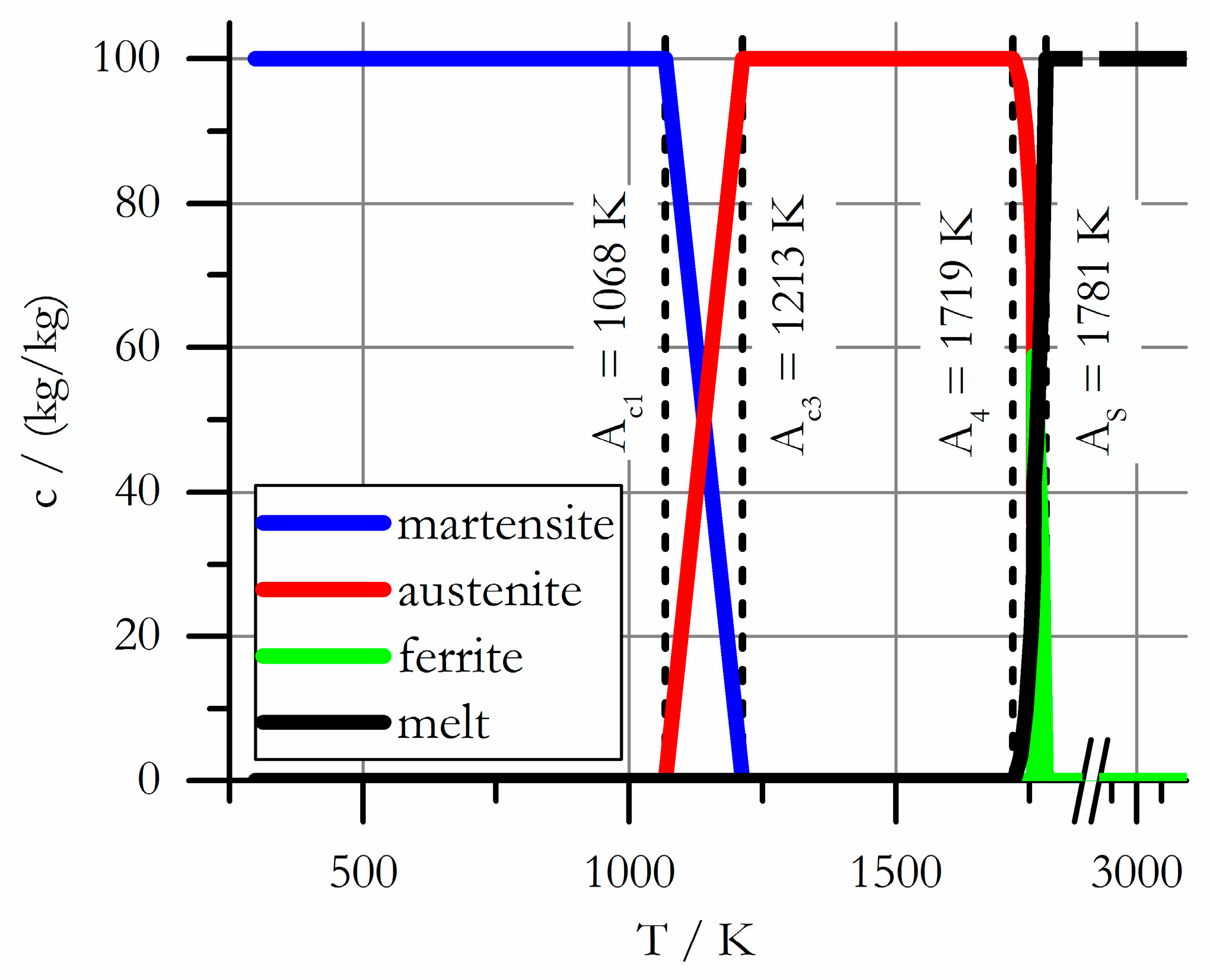
Figure 4.
Welding current program used in spot welding of 22MnB5.
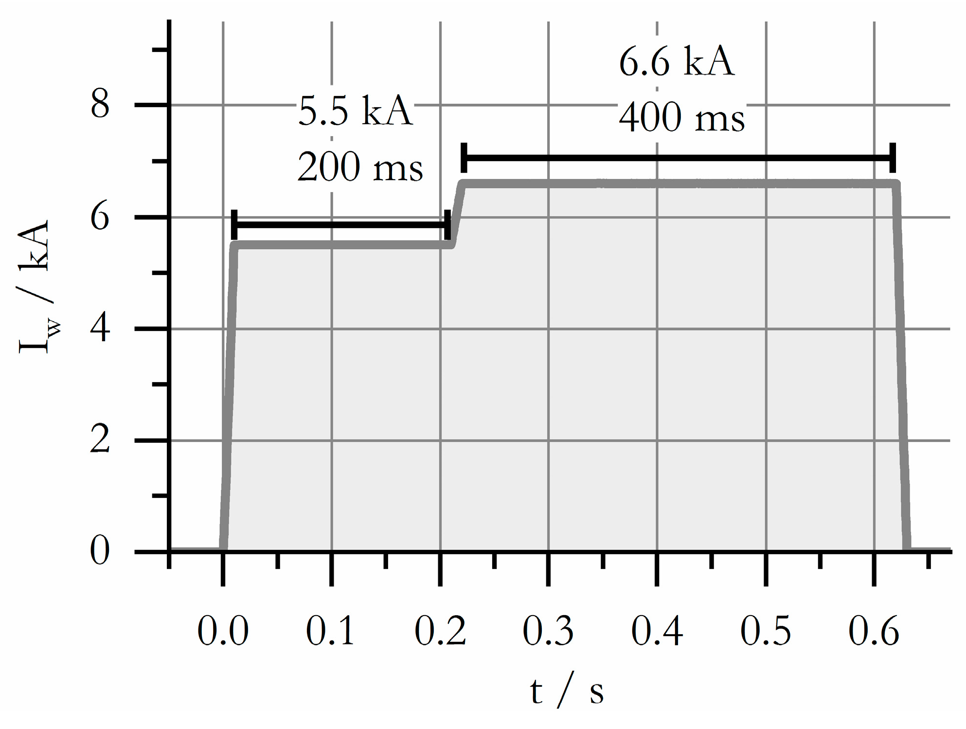
Figure 5.
Flow stress curves of 22MnB5 after rapid heating from heat-treated state; * artificial curves.
Figure 5.
Flow stress curves of 22MnB5 after rapid heating from heat-treated state; * artificial curves.
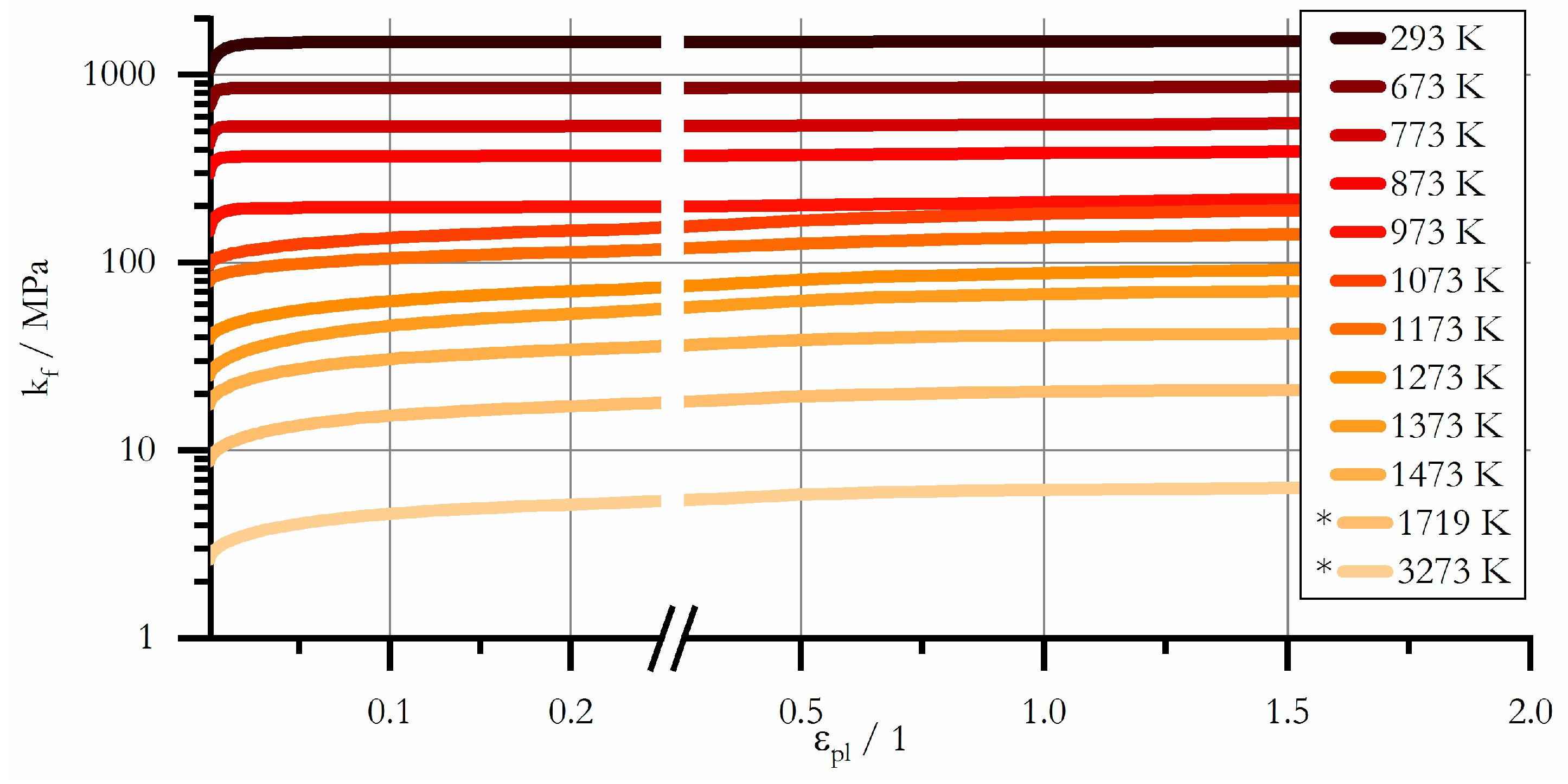
Figure 6.
Elastic modulus and Poisson ratio of 22MnB5.
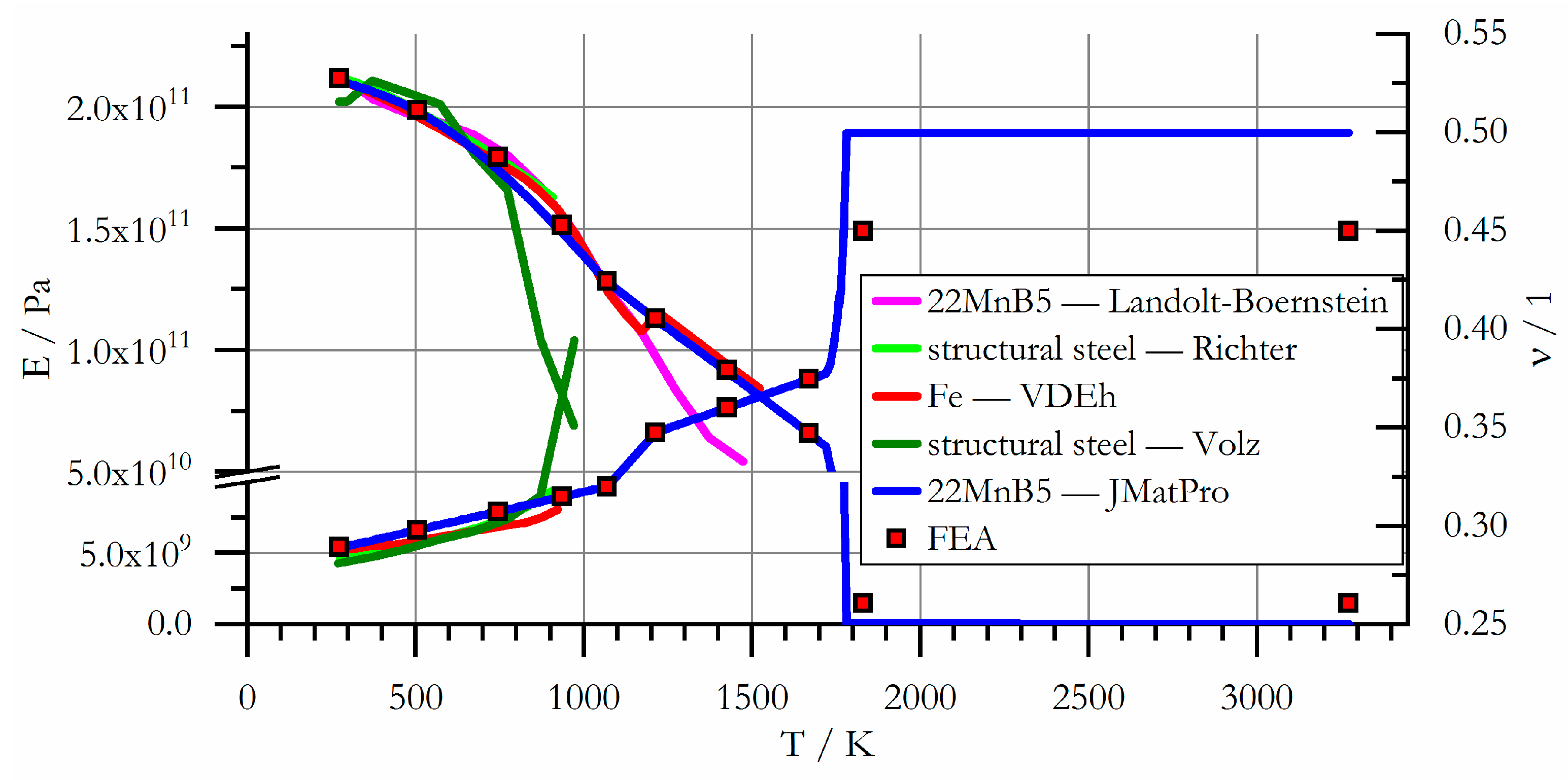
Figure 7.
Coefficient of thermal expansion of 22MnB5.
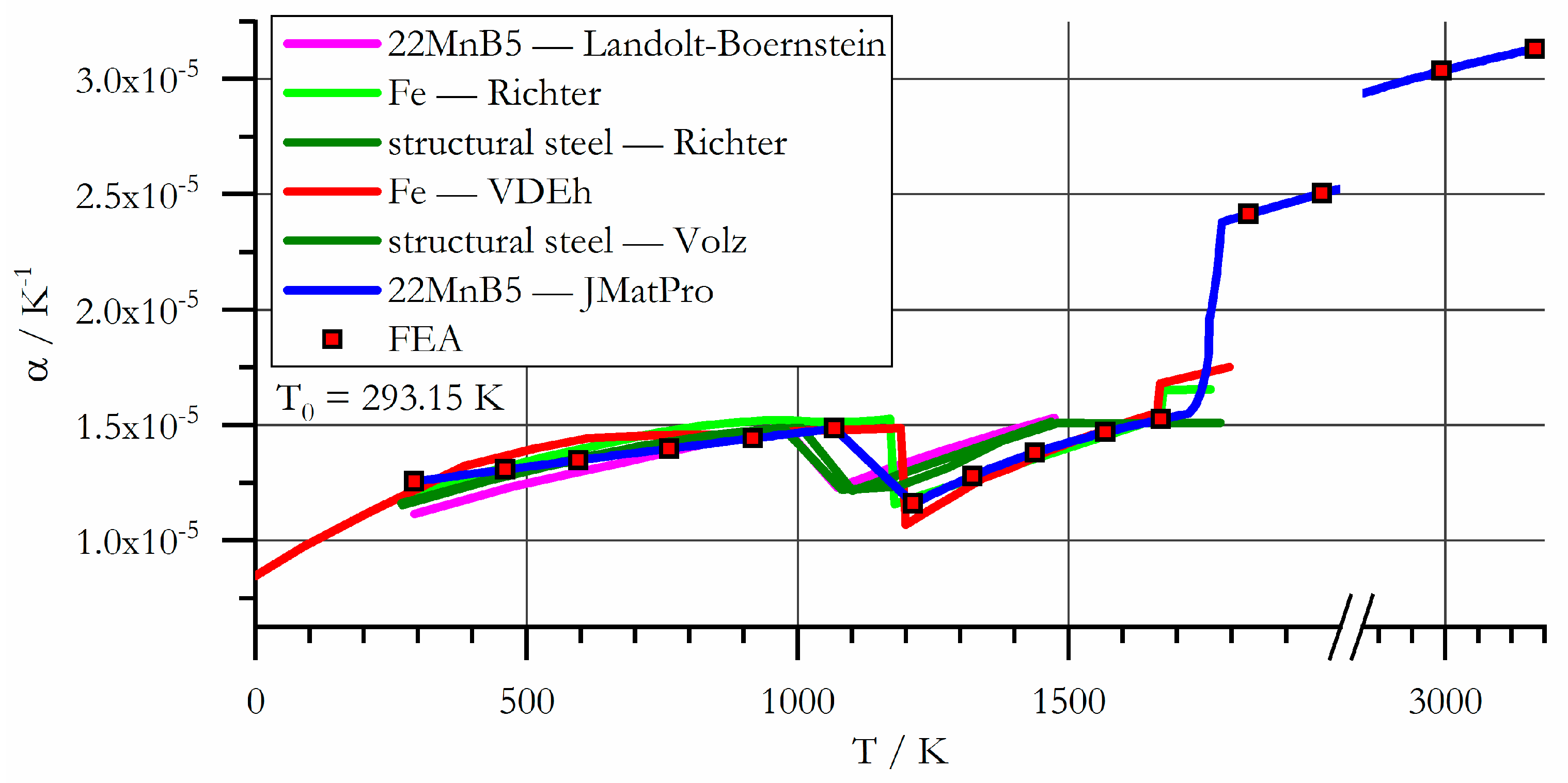
Figure 8.
Specific electric resistance of 22MnB5, literature data.
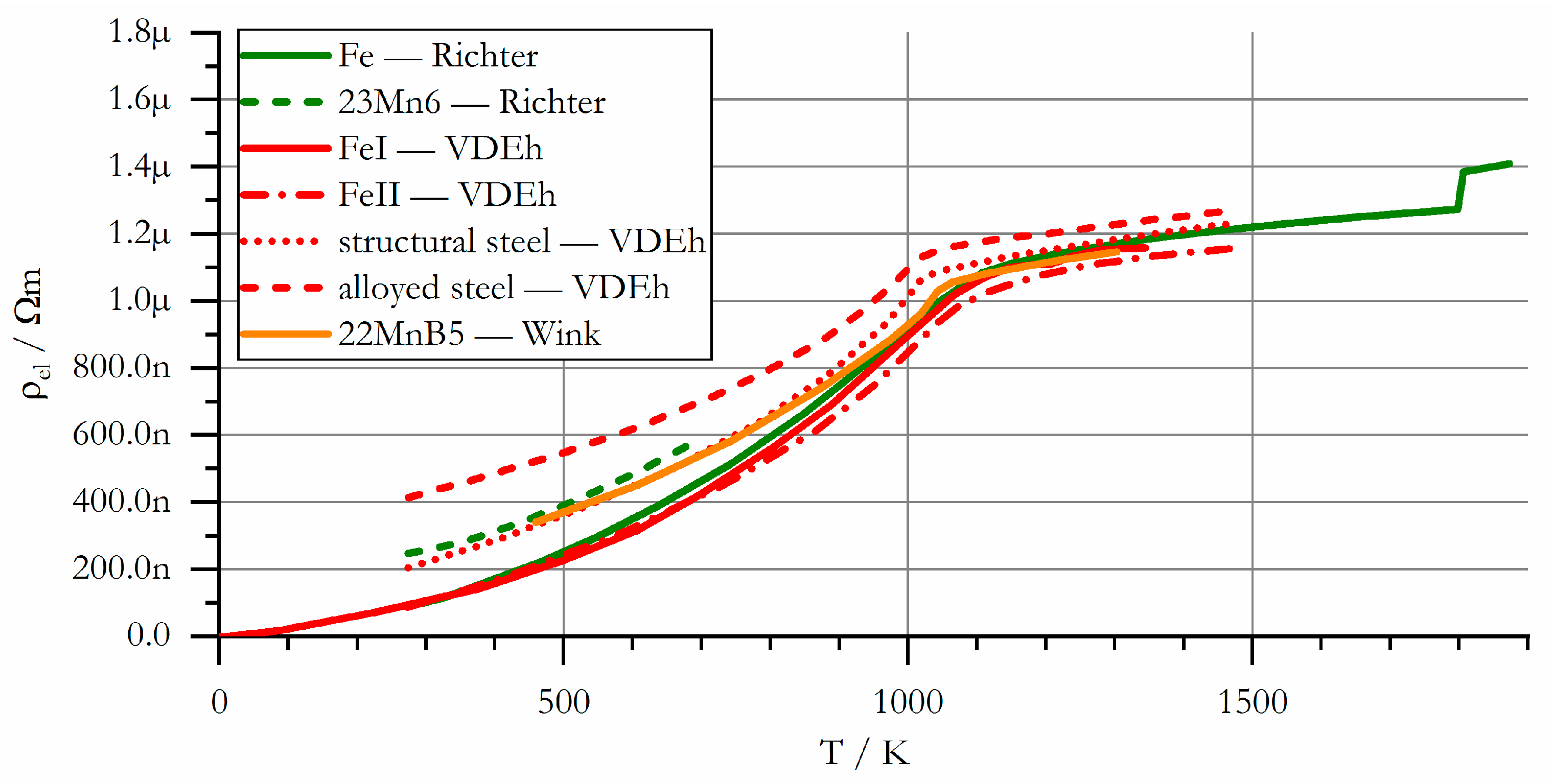
Figure 9.
Specific electric resistance of 22MnB5, computed data.

Figure 10.
Mass density of 22MnB5.
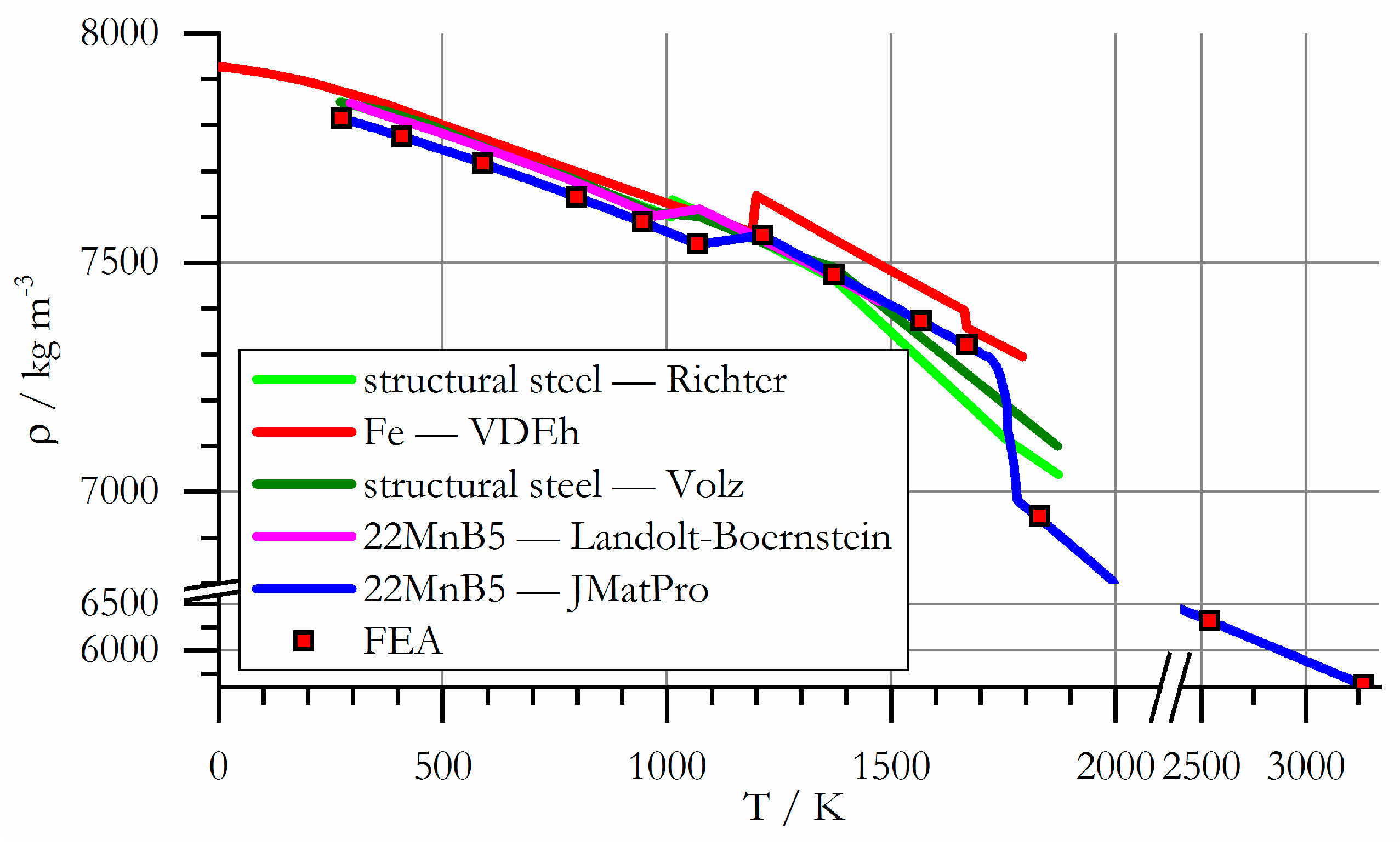
Figure 11.
Specific heat capacity of 22MnB5.

Figure 12.
Specific enthalpy density of 22MnB5.

Figure 13.
Specific thermal conductivity of 22MnB5.

Figure 14.
Macrosection of weld nugget in comparison to computed result, the latter half-translucent; temperature profile is in K, gray surface represents melt.
Figure 14.
Macrosection of weld nugget in comparison to computed result, the latter half-translucent; temperature profile is in K, gray surface represents melt.

Figure 15.
Nugget growth curve during the weld, measured and computed data.

Table 1.
Computed phase-transformation temperatures of 22MnB5; quasi-static according to [24], and rapid heating.
Table 1.
Computed phase-transformation temperatures of 22MnB5; quasi-static according to [24], and rapid heating.
| Quantity | ||
|---|---|---|
| 1153 | 1213 | |
| 993 | 1068 |
Table 2.
Hockett–Sherby flow stress parameters of 22MnB5 after rapid heating from martensitic state.
Table 2.
Hockett–Sherby flow stress parameters of 22MnB5 after rapid heating from martensitic state.
| 293 | 1066 | 1488 | 87 | 0.885 |
| 673 | 680 | 844 | 8934 | 1.533 |
| 773 | 432 | 529 | 818 | 1.11 |
| 873 | 298 | 368 | 134.5 | 0.82 |
| 973 | 147 | 196 | 90.5 | 0.83 |
| 1073 | 97 | 248 | 1 | 0.52 |
| 1173 | 79.5 | 180 | 1 | 0.515 |
| 1273 | 39 | 100 | 2 | 0.605 |
| 1373 | 25 | 74.3 | 2.6 | 0.663 |
| 1473 | 17.5 | 43.5 | 3 | 0.615 |
Table 3.
Physical properties of 22MnB5.
| 273.15 | 211.804 | 0.290 | 293.15 | 1.256 | 273.15 | 0.214 |
| 505.05 | 198.693 | 0.298 | 460.98 | 1.307 | 458.96 | 0.340 |
| 744.51 | 179.279 | 0.307 | 595.73 | 1.348 | 651.12 | 0.506 |
| 935.80 | 151.383 | 0.315 | 762.56 | 1.398 | 840.70 | 0.742 |
| 1068.15 | 128.226 | 0.320 | 917.37 | 1.442 | 1027.97 | 1.020 |
| 1213.15 | 113.060 | 0.347 | 1068.15 | 1.485 | 1068.15 | 1.082 |
| 1426.11 | 91.707 | 0.360 | 1213.15 | 1.160 | 1132.22 | 1.122 |
| 1669.15 | 65.859 | 0.375 | 1322.89 | 1.280 | 1244.72 | 1.156 |
| 1831.15 | 1.470 | 0.450 | 1437.27 | 1.380 | 1402.63 | 1.201 |
| 3273.15 | 1.470 | 0.450 | 1567.51 | 1.469 | 1570.86 | 1.238 |
| 1669.15 | 1.525 | 1669.15 | 1.254 | |||
| 1831.15 | 2.416 | 1831.15 | 1.402 | |||
| 1966.85 | 2.504 | 3273.15 | 1.604 | |||
| 2192.90 | 2.646 | |||||
| 2426.40 | 2.777 | |||||
| 2708.93 | 2.919 | |||||
| 2989.43 | 3.036 | |||||
| 3273.15 | 3.133 |
Table 4.
Physical properties of 22MnB5.
| 273.15 | 7815 | 273.15 | 0 | 273.15 | 45.738 |
| 408.21 | 7775 | 433.92 | 591 | 343.92 | 46.153 |
| 589.77 | 7717 | 637.68 | 1441 | 425.87 | 45.807 |
| 798.48 | 7643 | 735.55 | 1911 | 534.21 | 44.244 |
| 946.10 | 7588 | 851.72 | 2529 | 662.40 | 41.172 |
| 1068.15 | 7541 | 951.01 | 3150 | 854.26 | 35.678 |
| 1213.15 | 7560 | 1019.39 | 3652 | 956.06 | 33.161 |
| 1372.11 | 7475 | 1103.25 | 4163 | 1051.18 | 31.402 |
| 1566.58 | 7373 | 1213.15 | 4795 | 1150.47 | 29.447 |
| 1669.15 | 7322 | 1470.95 | 5921 | 1211.79 | 28.152 |
| 1831.15 | 6947 | 1669.15 | 6838 | 1407.03 | 30.473 |
| 2092.03 | 6722 | 1831.15 | 9110 | 1608.95 | 32.917 |
| 2539.46 | 6320 | 2022.07 | 9952 | 1669.15 | 33.700 |
| 3273.72 | 5625 | 2336.66 | 11,239 | 1831.15 | 100.000 |
| 2701.79 | 12,521 | 3273.15 | 120.000 | ||
| 3001.71 | 13,405 | ||||
| 3273.15 | 14,090 |
© 2018 by the authors. Licensee MDPI, Basel, Switzerland. This article is an open access article distributed under the terms and conditions of the Creative Commons Attribution (CC BY) license (http://creativecommons.org/licenses/by/4.0/).
Share and Cite
MDPI and ACS Style
Kaars, J.; Mayr, P.; Koppe, K. Determining Material Data for Welding Simulation of Presshardened Steel. Metals 2018, 8, 740. https://doi.org/10.3390/met8100740
AMA Style
Kaars J, Mayr P, Koppe K. Determining Material Data for Welding Simulation of Presshardened Steel. Metals. 2018; 8(10):740. https://doi.org/10.3390/met8100740
Chicago/Turabian StyleKaars, Jonny, Peter Mayr, and Kurt Koppe. 2018. "Determining Material Data for Welding Simulation of Presshardened Steel" Metals 8, no. 10: 740. https://doi.org/10.3390/met8100740
Note that from the first issue of 2016, this journal uses article numbers instead of page numbers. See further details here.