Numerical Simulation of the Depth-Sensing Indentation Test with Knoop Indenter


1
CEMMPRE—Department of Mechanical Engineering, University of Coimbra, Rua Luís Reis Santos, Pinhal de Marrocos, 3030-788 Coimbra, Portugal
2
Escola Superior de Tecnologia de Abrantes, Instituto Politécnico de Tomar, Rua 17 de Agosto de 1808—2200 Abrantes, Portugal
*
Author to whom correspondence should be addressed.
Metals 2018, 8(11), 885; https://doi.org/10.3390/met8110885
Submission received: 11 October 2018
/
Revised: 25 October 2018
/
Accepted: 26 October 2018
/
Published: 31 October 2018
(This article belongs to the Special Issue Modelling and Simulation of Sheet Metal Forming Processes)
Abstract
:Depth-sensing indentation (DSI) technique allows easy and reliable determination of two mechanical properties of materials: hardness and Young’s modulus. Most of the studies are focusing on the Vickers, Berkovich, and conical indenter geometries. In case of Knoop indenter, the existing experimental and numerical studies are scarce. The goal of the current study is to contribute for the understanding of the mechanical phenomena that occur in the material under Knoop indention, enhancing and facilitating the analysis of its results obtained in DSI tests. For this purpose, a finite element code, DD3IMP, was used to numerically simulate the Knoop indentation test. A finite element mesh was developed and optimized in order to attain accurate values of the mechanical properties. Also, a careful modeling of the Knoop indenter was performed to take into account the geometry and size of the imperfection (offset) of the indenter tip, as in real cases.
1. Introduction
Depth-sensing indentation (DSI) tests are typically used to evaluate the hardness and Young’s modulus of materials. They can also be used to extract the uniaxial mechanical properties of bulk and composite materials, such as the yield stress and the strain hardening parameter (see, e.g., [1,2,3,4]). The most common hardness testing methods were developed in the early twentieth century. They are typically performed using spherical, conical and pyramidal indenters with Vickers and Berkovich geometries. In addition, the Knoop pyramid geometry is also used [5].
Hardness tests with the Knoop indenter have been valuable in the mechanical characterization of some materials, such as thin coatings [6,7] and biological materials (e.g., dental tissue [8]). Another important application of this hardness tests is in the field of the gradient materials obtained by severe plastic deformation (see, e.g., [9,10,11]), for which it is required to determine the mechanical properties in thin samples and/or thin surface layers of the samples.
In fact, the Knoop indenter geometry leads to wider and shallower indentations for a given applied load than the Vickers and Berkovich geometries. This makes the Knoop hardness test particularly attractive in some cases as for the determination of the near-surface properties and the characterization of brittle materials. Moreover, the results obtained in the Knoop hardness test are sensitive to the indenter orientation, making it a useful tool to analyze the materials anisotropy (e.g., [12]).
Although Knoop indenter is relatively common to use, it has not received suitable attention with respect to the study of some of the peculiarities of the test itself. One of the first studies using numerical simulation of the Knoop indentation test was performed by Rabinovich and Sarin [13], in their study, the Knoop indentation was analyzed in the context of linear elasticity. Giannakopoulos [14] presented analytical results on the response of frictionless and adhesionless contact of flat, linear elastic and visco-elastic isotropic surfaces penetrated by pyramidal indenters including the Knoop geometry. Giannakopoulos and Zisis [15] studied the Knoop indentation of elastic and elastoplastic materials with and without strain hardening. More recently, Giannakopoulos and Zisis [16] presented a finite element study on the adhesionless contact of flat surfaces by Knoop indenter. Only a few experimental studies, such as those by Riester et al. [17,18] were performed in order to clarify the analysis procedure of DSI tests with the Knoop geometry. Recently, Ghorbal et al. [19] performed an experimental work on ceramic materials in order to compare the conventional Knoop and Vickers hardness.
In this context, the present study intends to contribute to clarify some aspects of the Knoop indentation, particularly those related to the analysis of depth sensing indentation (DSI) results. For this purpose, three-dimensional numerical simulations of the indentation tests were performed, using various pyramidal indenter geometries, from Vickers to Knoop. A systematic study is accomplished using materials with different mechanical properties whose ratio between the residual indentation depth after unloading and the indentation depth at maximum load is in the range . The correction factor, , required to determine the Young’s modulus, is evaluated as a function of the indenter geometry, from Vickers to Knoop. In addition, numerical simulations using flat indenters with equivalent lozenge geometries were performed, in order to better understand the role of the pyramidal geometry.
2. Theoretical Aspects
The ability of the ultramicrohardness equipment to register the load versus the depth indentation, during the test, enables us to evaluate not only the hardness, but also other properties, such as the Young’s modulus. Based on the Sneddon relationship [20] between the indentation parameters and Young’s modulus, Doerner and Nix [21] have proposed an equation that relates the Young’s modulus with the compliance, , of the unloading curve at the point of the maximum load and the contact area, , such as:
where is the geometrical correction factor for the indenter geometry. The specimen’s Young’s modulus, , is obtained using the equation:
where and are the Young’s modulus and the Poisson’s ratio, respectively, of the specimen (s) and of the indenter (i). When performing numerical simulations, the indenter can in a first approximation considered as rigid for simplicity (e.g., [22]), and so . The accuracy of the Young’s modulus results, obtained with the above equations, depends on the correct evaluation of the contact area and compliance. The contact area, , can be evaluated by two different procedures. One procedure uses the contour of the indentation in the finite element mesh, in order to make the results independent of the formation of pile-up or sink-in. The other is the usual experimental procedure, which makes use of the compliance, , evaluated by fitting the unloading part of the load–indentation depth curve, (P − h), using the power law [22]:
where T and m are constants obtained by fit and is the lower value of the indentation depth, h, used in the fitted region, corresponding to a load value , during unloading. The upper part of the unloading curve taken into account in the fits is 70% [22]. Once the value of compliance, , is known, the contact indentation depth, , that allows the calculation of the contact area according to the geometry of the indenter , is determined by the equation , where is the indentation depth at the maximum load, , and is a parameter equal to 0.72 for conical or pyramidal (Berkovich [23], Vickers [22] and Knoop [18] indenters).
An approach that can be used for evaluating the correction factor, , was proposed by Joslin and Oliver [24], combining the hardness and Young’s modulus equations:
where is the hardness, P the maximum applied load and the stiffness . The ratio between the maximum applied load and the square of the stiffness, , is an experimentally measurable parameter that is independent of the contact area and so of the penetration depth [24].
3. Numerical Simulation and Materials
Three-dimensional numerical simulations of the hardness tests were carried out, using a finite element (FE) in-house code DD3IMP. This FE code, which has already been tested in the case of Vickers, Berkovich and conical indentation of bulk materials and thin films (see, e.g., [22,25,26]), allows simulating the hardness tests with any type of indenter shape, taking into account contact with friction between the indenter and the sample [22,27,28]. The mechanical model, which is the basis of the DD3IMP code, considers the hardness test as a quasi-static process that occurs in the large plastic deformations domain. In DD3IMP, the contact with friction problem is modeled using a classical Coulomb’s law. To relate the static equilibrium problem to the contact with friction, an augmented Lagrangean method is applied to the mechanical formulation. This leads to a system of non-linear equations, where the kinematic (material displacements) and static variables (contact forces) are the final unknowns [27,28]. To solve this problem, the code uses a fully implicit Newton–Raphson-type algorithm. All non-linearities, induced by the elastoplastic behavior of the material and by the contact with friction, are treated in a single iterative loop [27,28].
In the current study, the friction between the indenter and the deformable body was assumed to have a friction coefficient of 0.16. This is a commonly used value and leads to a better description of the indentation process than if frictionless contact is assumed [22,26].
3.1. Indenters
The Knoop indenter has a pyramidal geometry, with a lozenge-shaped base having one diagonal (L) 7.11 times longer than the other (m). The angles between the edges (apical angles) are for the long edges and for the short edges, as shown in Figure 1.
The ideal (in the absence of pile-up or sink-in) indentation contact area, , of the Knoop indenter as function of the indentation contact depth is given by:
where is the ideal indentation contact depth, and are the semi-apical angles of the Knoop indenter.
The Knoop indenter geometry was modeled using parametric Bezier surfaces, which allows a satisfactory description of the indenter tip, namely an imperfection such as occurs in the real geometry, similar to the case of offset in the Vickers indenter [25,29]. The modeled Knoop indenter, shown in Figure 2, has a tip imperfection consisting of a plane normal to the indenter axis with an area equal to (this value is the same as the experimentally found, for the Vickers indenter, by Antunes et al. [29]).
Due to the tip imperfection, the indenter area function does not match the ideal area function above mentioned (Equation (5)). Table 1 shows the area function of the Knoop indenter (ratio, R = L/m = 7.11) used in the numerical simulations. This table also shows four others area functions of pyramidal indenters, used in this study, with different values of the ratio, R, between the diagonals of the indenter (R = 1, 2.5, 4 and 5.5), where the ratio R = 1 corresponds to the Vickers indenter.
For pyramidal indenters, other than Vickers and Knoop, the angles and were chosen such that the tangents of and follows a quasi-linear evolution with R, as shown in Figure 3. In this way it is possible to study the extent to which the deviation of Vickers geometry towards the Knoop geometry influences the indentation results obtained with DSI experiments.
In order to better understand some aspects related with the influence of the indenter geometry on the mechanical properties evaluation, numerical simulations using lozenge-shaped flat indenters were also performed. The flat indenters were modulated with five values of the ratio, R = L/m, between the diagonals of the lozenge, as for the pyramidal indenters (R = 1, 2.5, 4, 5.5, and 7.11).
3.2. Finite Element Mesh
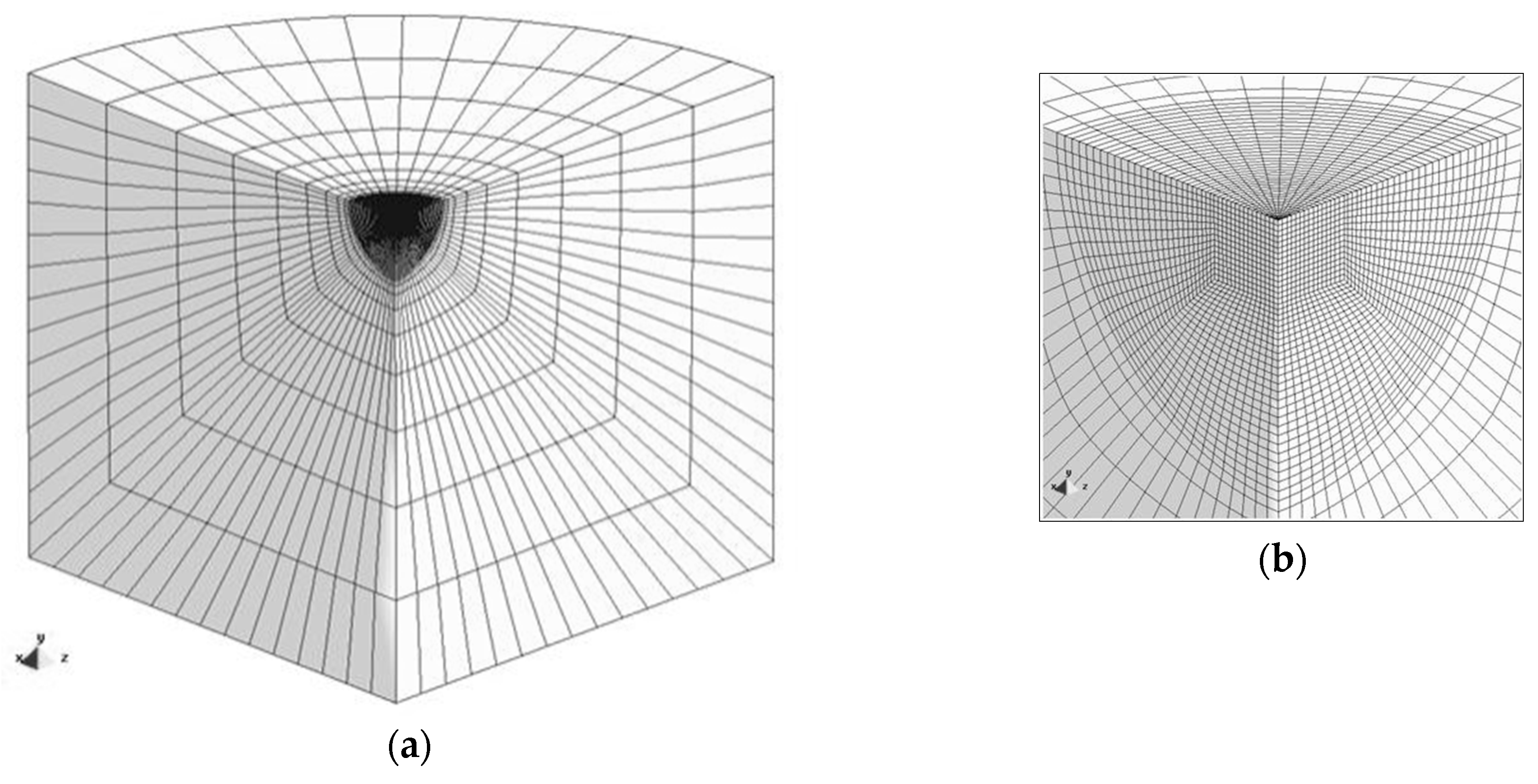
The test sample used in the numerical simulations has both radius and thickness equal to 40 µm. Its discretization was performed using three-linear eight-node isoparametric hexahedrons. Due to geometrical and material symmetries in the X = 0 and Z = 0 planes, only a quarter of the sample was used in the numerical simulation, as shown in Figure 4.
The FE mesh is composed by 17,850 elements. The size of the elements in the indentation region is . This refinement has proven to provide accurate values of the indentation contact area, when measured using the contour of the indentation, in case of Vickers and Berkovich geometries, with equal value of offset area (see, e.g., [22,26]). In fact, the Young’s modulus values obtained from the indentation contact area, evaluated using the contour of nodes in the FE mesh in contact with the indenter at maximum load presents an error less than 1%, when compared with the values used as input in the numerical simulation (e.g., [26]). In the present study, the size of the central region of the finite element mesh, especially refined, is larger than in these cases, and thus the total number of elements is approximately three times greater, in order to take into account the elongated geometry of the Knoop indenter.
3.3. Materials
Three-dimensional numerical simulations of depth-sensing indentation with pyramidal indenters were carried out using 45 fictitious materials, whose mechanical properties are shown in Table 2. In order to cover a wide range of materials used in engineering applications, five values of yield stress (0.2, 2, 6, 10, and 20 GPa), three values of Young’s modulus (70, 200 and 400 GPa) and of strain hardening parameter of the Swift law (0.01, 0.15 and 0.3), were taken into account.
The plastic behavior of the materials is described by the von Mises yield criterion and the Swift hardening law: where and are the equivalent stress and plastic strain, respectively, and , and n (strain hardening coefficient) are the material parameters (the yield stress is: ); the parameter was considered to be equal to 0.005. The elastic behaviour is isotropic and described by the generalised Hooke’s law; the Poisson’s ratio, is 0.3, for all simulations.
4. Results
4.1. Indentation Geometry and Equivalent Plastic Strain Distributions
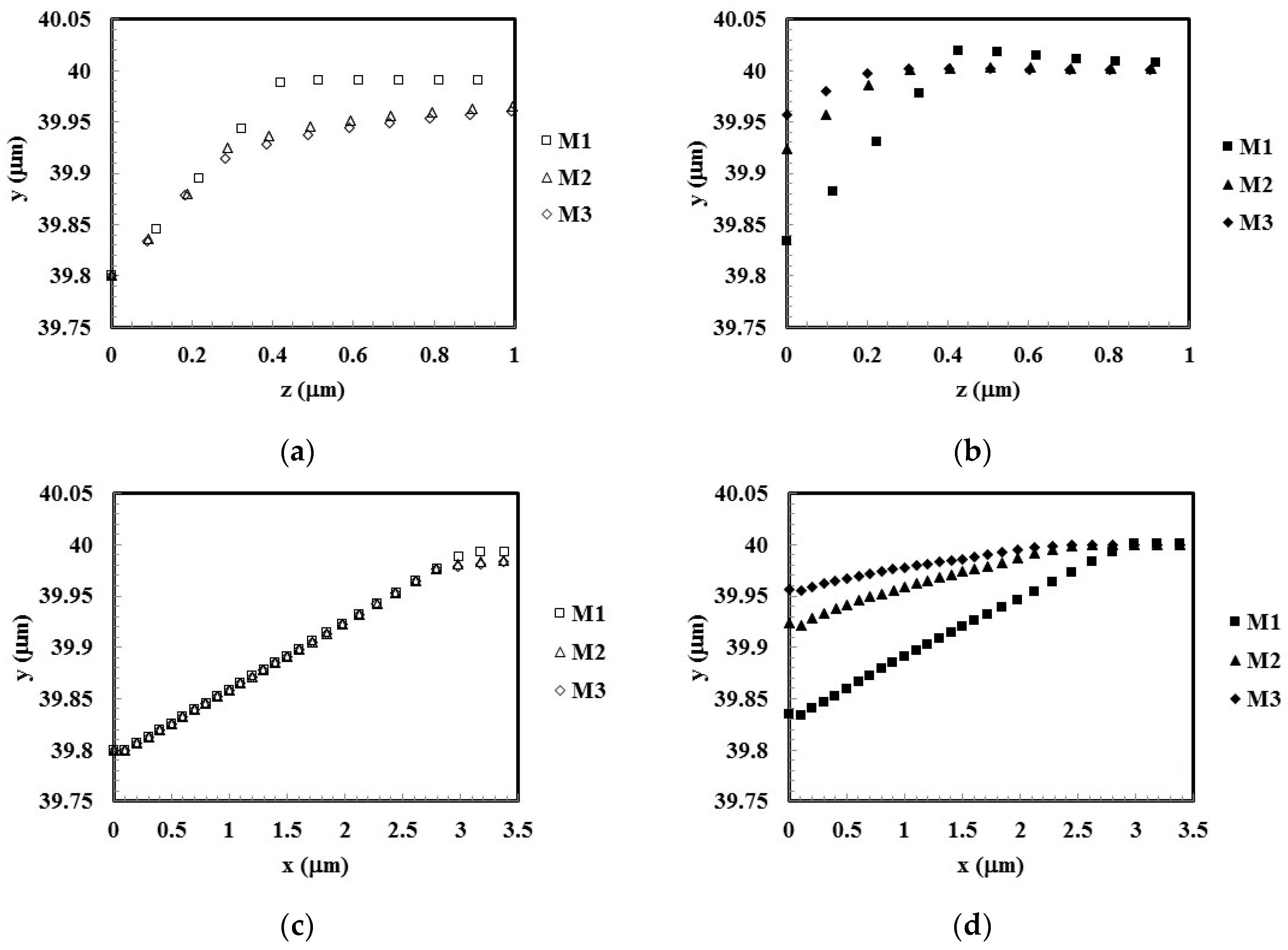
A study of the indentation geometry with the Knoop indenter (R = 7.11) was performed using only three of the materials in Table 2, covering different values in the possible range of . Table 3 shows the mechanical properties of these materials, which have two Young’s modulus values, 200 and 400 GPa, yield stress of 0.2, 6, and 20 GPa, and two values of the strain hardening parameter, n ≈ 0 and n = 0.3. Table 3 also includes the value of the ratio between the indentation depth after unloading and the indentation depth at maximum load, . This ratio, which can be easily obtained from the experimental load-unloading curve, is independent of the maximum indentation depth, for a given material in cases of conical [30] and Vickers [22] indentations. Its range of values is from 0 to 1, which corresponds to materials with purely elastic and rigid-plastic behaviors, respectively. All numerical simulations of the hardness test were performed up to the same maximum indentation depth, .
Figure 5 shows the indentation profiles, obtained for the three materials at maximum load (Figure 5a,c) and after unloading (Figure 5b,d), along the two diagonals, the shorter, m, and the longer, L, respectively. Figure 5a shows that for the shorter diagonal, the indentation profile obtained at the maximum load depends on the material mechanical properties. In case of materials M2 and M3 the indentation surface sink-in. This behavior can be associated with the value of the ratio that is equal to 0.40 and 0.25 (for the materials M2 and M3, respectively), and with the high value of the strain hardening parameter, n. In case of M1 material, with a ratio equal to 0.97, i.e., close to 1, the indentation surface does not present sink-in or pile-up. On the other hand, the indentation profile obtained at maximum load for the longer diagonal, almost does not depends on the materials mechanical properties (Figure 5c).
After unloading, the indentation profiles corresponding to the materials M2 and M3 shown elastic recovery in both diagonals (Figure 5b,d). Moreover, the amount of elastic recover increases with the decrease of the ratio . In case of M1 material, with a ratio and without strain hardening, the indentation profile along the short diagonal shows pile-up (Figure 5b). In fact, for other indenter geometries (conical and Vickers), the pile-up appears for values of the ratio higher than 0.8 in materials without strain hardening (see, e.g., [22,30]). It should be noted that, for a given material, the ratio correlates with the value of the H ratio between the hardness and the Young’s modulus, and slightly depends on the strain hardening parameter.
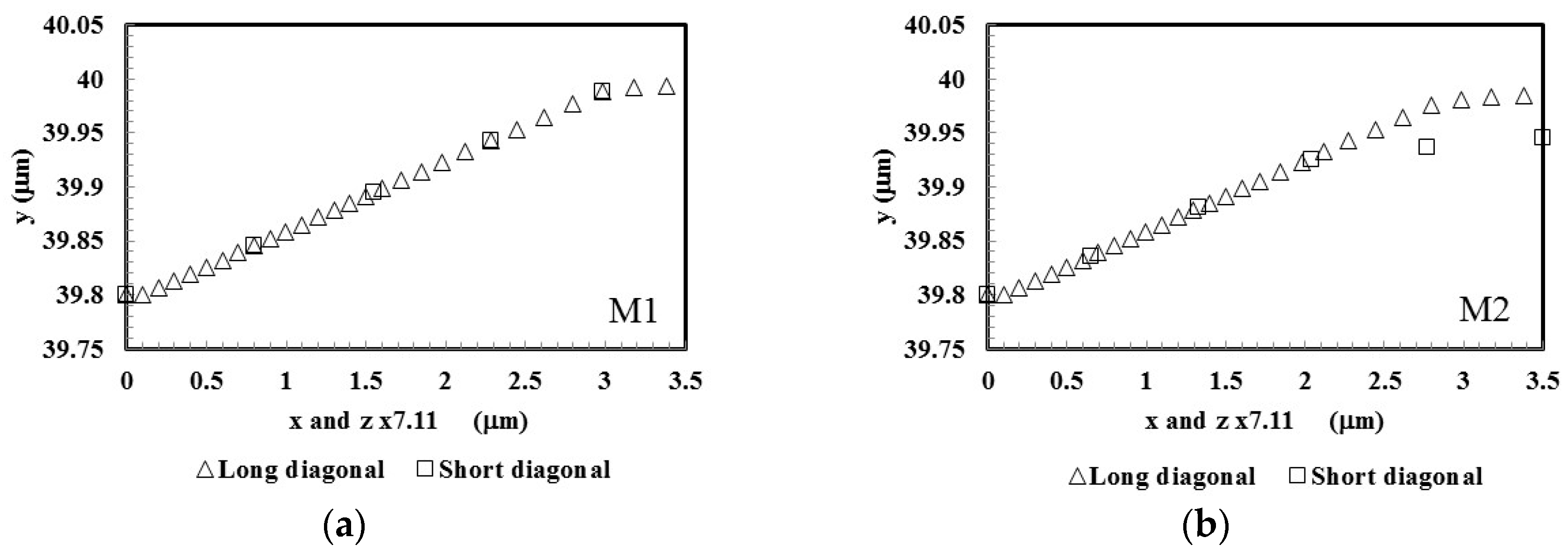
Figure 6 shows the comparison between the Knoop indentation diagonals at maximum load. To make possible this comparison, the indentation profiles were normalized by considering the value of the R-ratio between the indenter diagonals (R equal to 7.11). Figure 6a shows that in the material M1 the two diagonal exhibit a similar behavior. In the case of the materials M2 and M3 sink-in is observed along the short diagonal. Moreover, the sink-in slightly increases with the value of the ratio .
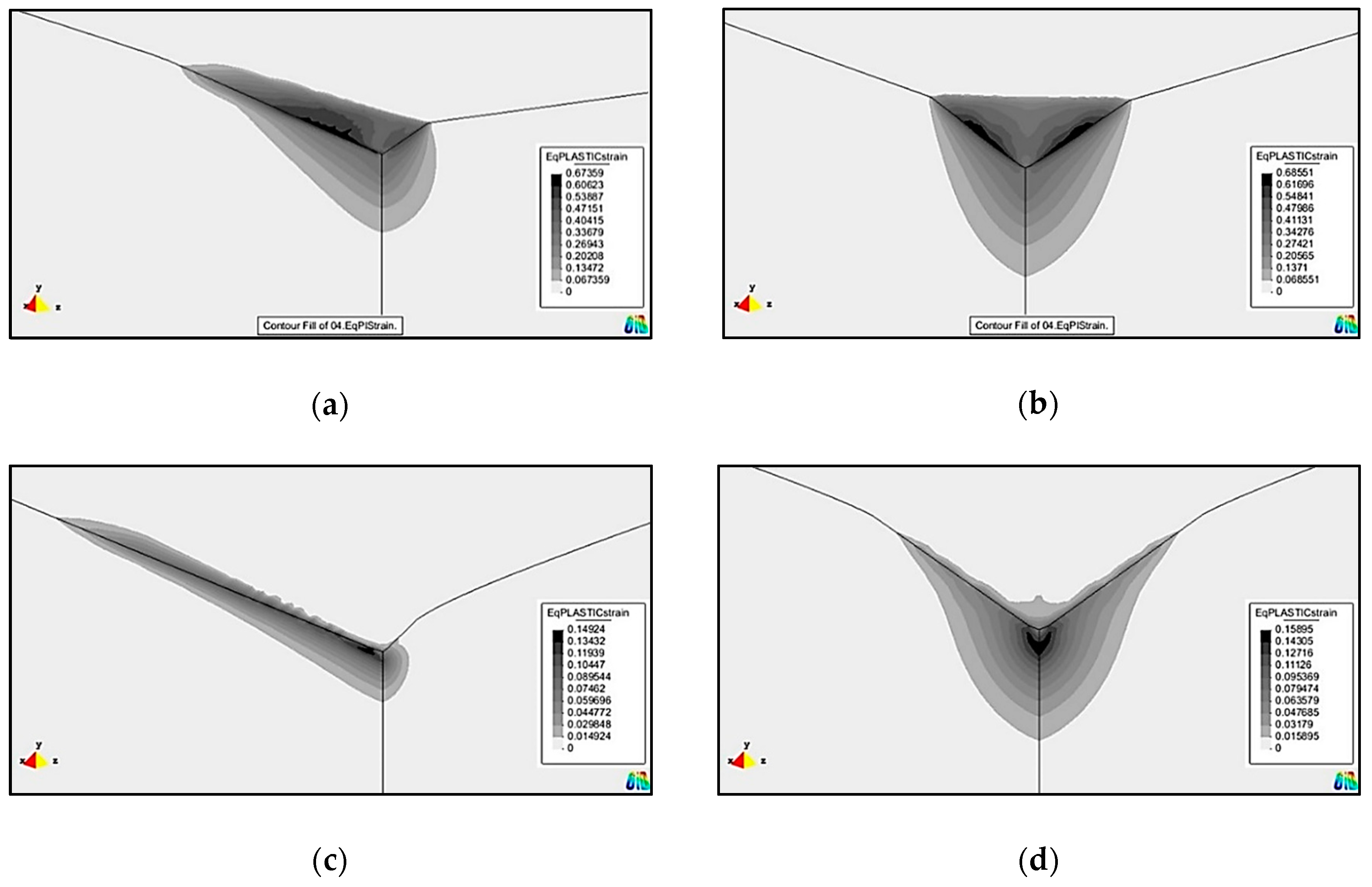
The effect of the indenter geometry on the equivalent plastic strain distribution of the indentations was also studied. Figure 7a,c shows the equivalent plastic strain distributions obtained at the maximum load in the numerical simulations of the materials M1 () and M3 using the Knoop indenter. For comparison, the same figure also shows the same distributions obtained with the Vickers indenter (Figure 7b,d).
For each material, the maximum values of the equivalent plastic strain are quite similar for the Knoop and Vickers indenters. However, in the case of Knoop, the equivalent plastic strain distributions are asymmetric with respect to the indenter axes. The maximum values of the equivalent plastic strain are observed along the longest diagonal. For M1 material (), the maximum value of the equivalent plastic strain is slightly higher in the Vickers indentation (≈0.686) than for Knoop (≈0.674). The maximum plastic strain region is located just at the surface in the edge regions of the indentation (Figure 7a,b). In case of the M3 material , as shown in Figure 7c,d, the maximum value of equivalent plastic strain is also somewhat higher for the Vickers indentation (≈0.159), than for the Knoop (≈0.149). However, for this material, the region with maximum equivalent plastic strain is located beneath the indentation surface, whatever the indentation geometry.
4.2. Indentation Contact Area and Young’s Modulus
The results of the numerical simulation of the hardness tests with the Knoop indenter, for all materials in Table 2, were used to study the influence of the mechanical properties on the evaluation of the indentation contact area and, consequently, on the Young’s modulus. As mentioned above, the indentation contact area was determinate using two different procedures: one of them uses the load-unloading curve as in the experimental DSI procedure for evaluating this area, , and the other considers the contour of nodes of the FE mesh in contact with the indenter at maximum load, (numerical contact area).
Figure 8 shows the evolution of the indentation contact areas, and , as a function of the ratio . These contact areas are normalized with respect to the reference area, , corresponding to the obtained with the area function of the indenter (Equation (5), with equal to the indentation depth, which does not take into account the pile-up or sink-in formation). Figure 8a shows that the contact area, , is independent of the strain hardening parameter and Young’s modulus, whatever the value of the ratio . Moreover, the ratio is always less than 1. Figure 8b shows that the numerically calculated contact area, , is nearly independent from the strain hardening parameter and Young’s modulus, for the ratio . However, for the normalized contact area depends on the strain hardening parameter. The ratio is even higher than 1 after a value of that depends on the strain hardening parameter ( equal to 0.85, 0.90 and 0.95 for n equal to 0, 0.15 and 0.3, respectively), indicating pile-up formation. For both cases, and , similar behaviors were previously observed for the case of the conical, Vickers and Berkovich indenters (see, e.g., [22,26,30]).
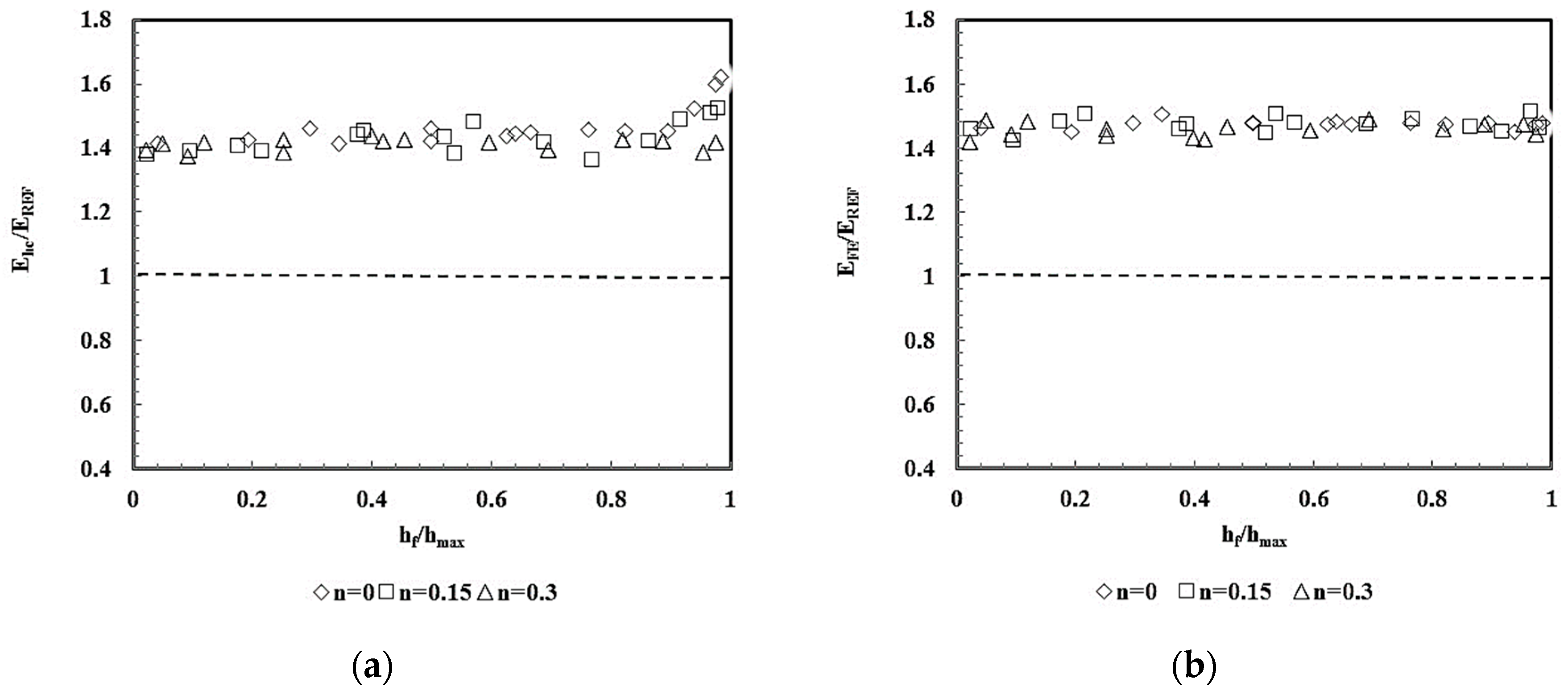
Figure 9 shows the evolution of the Young’s modulus and normalized by the input value used in the numerical simulation, , as a function of the ratio . The average ratio of is close to 1.419, except for values of approaching 1, for which the ratio increases for low values of the strain hardening parameter of the materials (n = 0 and 0.15). This is a consequence of the pile-up formation during the indentation of these materials, as was also observed for Vickers indenters [25]. The ratios of are slightly higher than those of , being in average close to 1.469. Slight differences between both ratios, and , were already observed for the Vickers indenter [25]. Under these conditions, in the experimental indentation tests, a value for the correction factor of 1.419 is required to be used for the contact area evaluation () from the unloading curve, in case of the Knoop indentation. This value is essentially different from other indenter geometries such as conical, Vickers and Berkovich, which require values around 1.034, 1.055, 1.081, respectively (see, e.g., [22,26]).
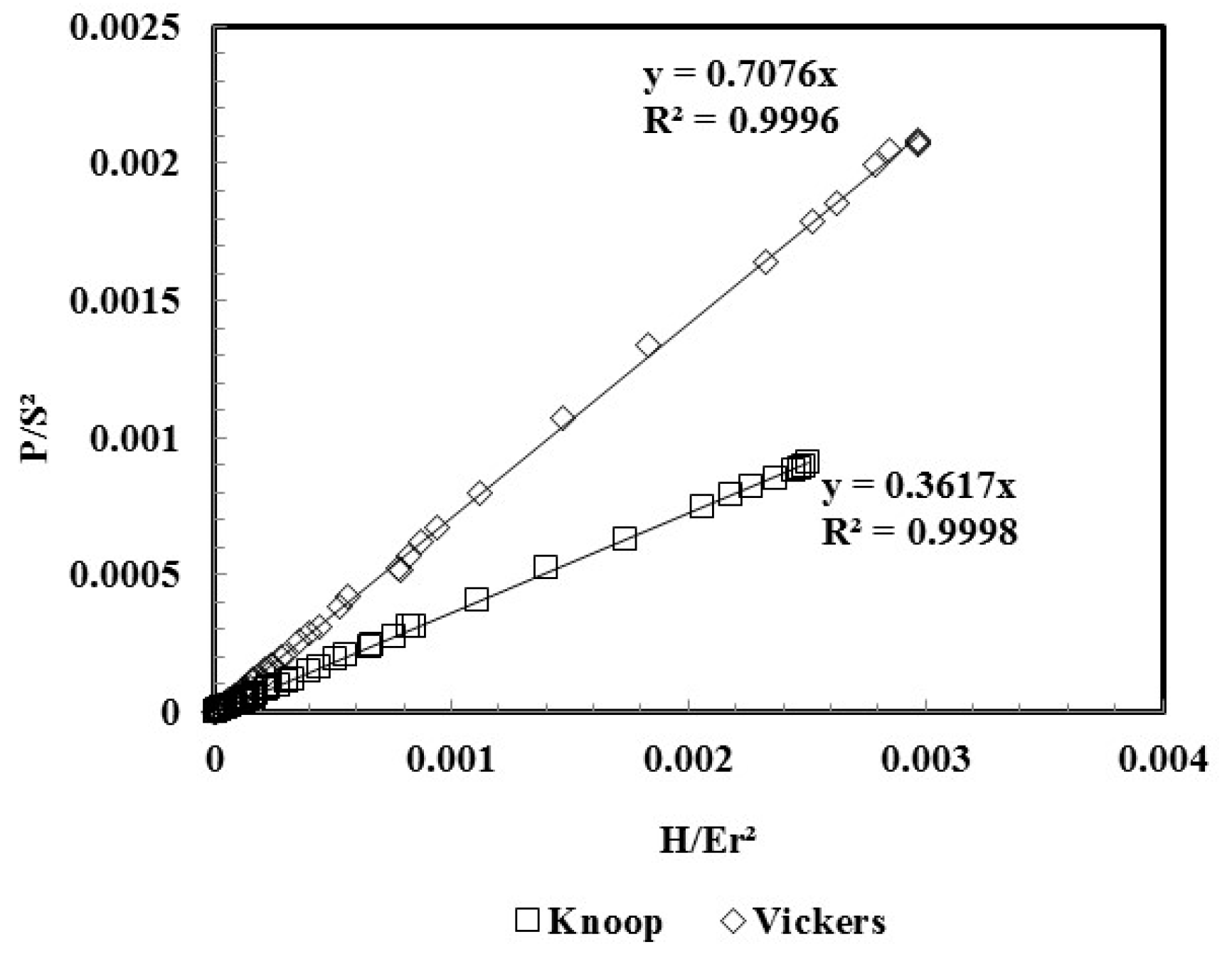
Equation (4) was used in order to confirm the above correction factor . Figure 10 shows the ratio versus obtained by numerical simulation of all materials in Table 2, for the case of the Knoop and Vickers indenters. The reduced Young’s modulus, , was determined considering the input Young’s modulus and Poisson ratio, , determined using the contact area evaluated from the contour of the indentations.
The straight-lines in Figure 10 pass through the origin of the axes as indicated by Equation (4) (independently of the indenter geometry, curves match for E, i.e., for materials with rigid-plastic behaviour, which corresponds to the ratio ). The factor is evaluated from the slope, , of the straight line, related with through . Using this procedure, for the values of the R-ratio of 1, 2.5, 4, 5.5, and 7.11, the correction factor obtained were 1.054, 1.141, 1.232, 1.351, and 1.473, respectively. The value of 1.473 for the Knoop indenter is very close to that mentioned above (1.469), obtained from the ratios (Figure 9b).
4.3. Flat Indenter
In order to understand if the value of the factor is affected by the plastic deformation beneath the indenter, five flat-ended punches were considered having the same R-ratio values between the diagonals (L and m) as for pyramidal indenters (Table 1). Also, the flat-ended punches were modeled using parametric Bezier surfaces and the finite element mesh is shown in Figure 4. This study allows an understanding of to what extent the evolution of the factor values with R is related to the pyramidal geometry of the indenter and/or to the loss of symmetry of the flat punches, when R evolves from 1 to 7.11.
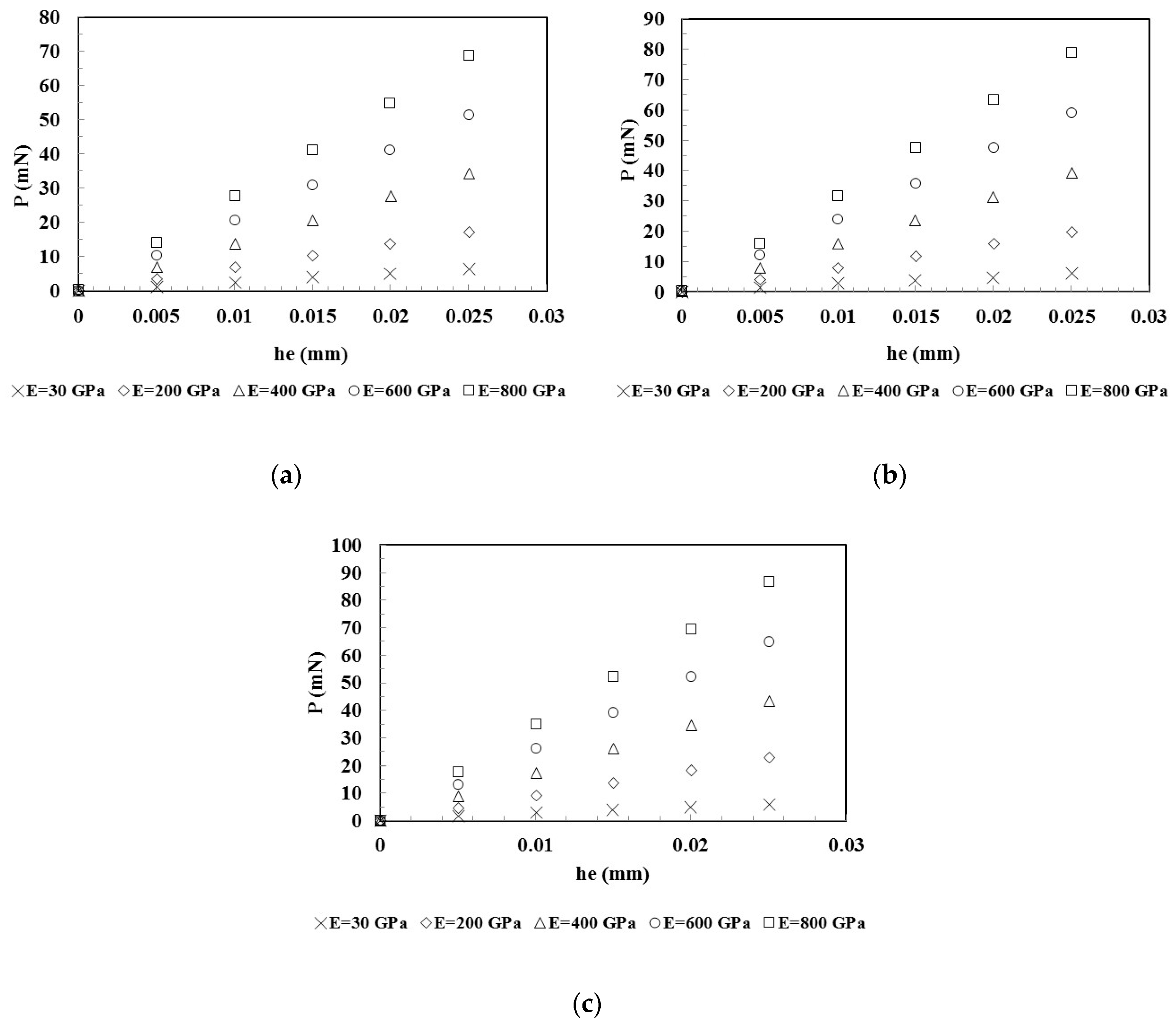
Using flat indenters, numerical simulations were performed up to a displacement imposed so that only elastic deformation occurs in the material beneath the indenter. Five values of Young’s modulus were used: 30, 200, 400, 600 and 800 GPa. Figure 11 shows the evolution of the load as a function of the indentation depth, , obtained in the numerical simulations with the flat indenters for values of the R-ratio equal to 1 (as for the Vickers indenter), 4 and 7.11 (as for the Knoop indenter). The figure shows that, for a given indentation depth, the load increases with the increase of the Young’s modulus and the R-value.
As above mentioned, Equation (1) comes from the Sneddon’s equation [20] that relates the applied load, P, with the elastic deflection of the surface of the material, , and can be written as follows:
where and are de Young’s modulus and Poisson ratio of the material, respectively; a is the radius of the rigid Sneddon cylindrical flat indenter, or an equivalent value for other rigid indenter geometry with the same area; and is a parameter that takes into account the geometry of the indenter (, for cylindrical flat indenter).
The Young’s modulus results obtained by the data such as in Figure 11 indicate that, in case of the flat punches, the value of the parameter in Equation (6) is different from 1 and depends on the R-ratio, whatever the Young’s modulus, as shown in Table 4.
The values of for R = 1 (as for the Vickers indenter) is in agreement with those obtained in previous studies (see, e.g., [22,26]). In the case of R = 7.11 (as for the Knoop indenter), is equal to 1.372. The increase of the value of with R is certainly related with the loss of symmetry of the flat punches with the increase of the ratio R. Indeed, the same was observed in case of the conical, Vickers and Berkovich indenters, whose values of the factor increase in this order (1.034, 1.055, 1.081, respectively), although on a smaller scale [26].
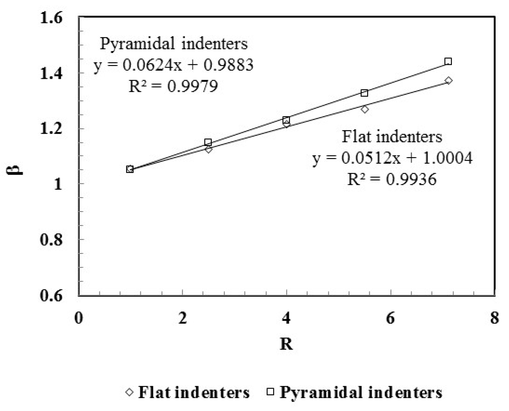
Figure 12 shows that the evolution of with R for the flat punches is a quasi-linear function, quite close to that observed for the case of the pyramidal indenters (obtained with Equation (4): 1.054, 1.141, 1.232, 1.351 and 1.473). Moreover, the values of for the pyramidal indenters are slightly higher than those determined for the flat indenters, except the R-ratio equal to 1.
The dissimilarity between the values obtained for the flat and the pyramidal indenters is certainly because, in the case of pyramidal indenters, not only elastic deformation occurs, but also plastic deformation appears, which significantly distorts the material surface. Moreover, the increase of the value of R-ratio leads to the lowering of the symmetry of the plastic strain distribution along two axes of the indenter (see Figure 7).
4.4. Correlation with Experimental Results
In order to check the performance of the correction factor proposed in this study, experimental results of five materials were used to calculate the Young’s modulus. They are fully dense brittle materials, covering a wide range of mechanical properties, whose experimental data were obtained from bibliography [19]. Table 5 presents the Young’s modulus results of these materials determined by Grobal et al. [19], using two different methods proposed by: (i) Grobal et al. [19] (); (ii) and Marshall et al. [31] and Riester et al. [18] (). The results obtained by the method proposed in the current study (), using equal to 1.419 as defined above for the Knoop indenter, are also shown in this table. For comparison, nominal values of the Young’s modulus, , evaluated by ultrasonic method [19] are presented and used to calculate the errors. To evaluate the Young’s modulus, Grobal et al. [19] make use of the plot of the contact stiffness, C, as a function of , whose values of the slopes of the fitted straight lines ( in Equation (1)), are also used in current study to assess the value of , for all materials.
The results in Table 5 show that the proposed coefficient enables relatively good accuracy of the Young’s modulus. The average of the absolute value of the error is equal to 4.27%. This is higher than that obtained by the method of Grobal et al. [19] and slightly lower than that achieved using the method by Marshall et al. [31].
5. Conclusions
A finite element study using the three-dimensional numerical simulation of hardness tests of elastic–plastic materials is performed. Pyramidal indenters with geometry from Vickers to Knoop were used. Also flat-ended punches were considered. This allowed us to obtain important information about the geometry of the indentation surface (sink-in and pile-up formation) and the distribution of plastic deformation beneath the pyramidal indenters. Both types of tests, with pyramidal and flat punch indenters, allow an assessment of the values of the geometrical parameter to be used in the Sneddon’s equation [20], for flat-ended punches, and the Doerner and Nix equation [21], for pyramidal indenters. This permits to determine the reduced Young’s modulus of the indented material when using depth-sensing indentation (DSI) equipment. In the case of the Knoop indenter, the correction factor of at about 1.419 is required, in order to accurately obtain the Young’s modulus. This makes the procedure for analyzing the results of the Knoop indenter more expeditious than it currently is.
Author Contributions
M.I.S. carried out the numerical simulations, with the support of N.A.S.; M.I.S., J.M.A., J.V.F. and N.A.S. performed the formal analysis; J.M.A. wrote the original manuscript; all the authors participate in the writing-review and editing process.
Acknowledgments
This research work is sponsored by national funds from the Portuguese Foundation for Science and Technology (FCT) via Projects UID/EMS/00285/2013 and CENTRO-01-0145-FEDER-000014 (MATIS), by UE/FEDER funds through Program COMPETE2020. One of the authors, N. A. Sakharova, was supported by a grant for scientific research from the Portuguese Foundation for Science and Technology (SFRH/BPD/107888/2015). All supports are gratefully acknowledged. The authors also express their thanks to Professor Marta Oliveira for her support in numerical simulation with the finite element in-house code DD3IMP.
Conflicts of Interest
The authors declare no conflict of interest. The funders had no role in the design of the study; in the collection, analyses, or interpretation of data; in the writing of the manuscript, or in the decision to publish the results.
References
- Fernandes, J.V.; Trindade, A.C.; Menezes, L.F.; Cavaleiro, A. Influence of substrate hardness on the response of W-C-Co-coated samples to depth-sensing indentation. J. Mater. Res. 2000, 15, 1766–1772. [Google Scholar] [CrossRef]
- Dao, M.; Chollacoop, N.; Van Vliet, K.J.; Venkatesh, T.A.; Suresh, S. Computational modelling of the forward and reverse problems in instrumented sharp indentation. Acta Mater. 2001, 49, 3899–3918. [Google Scholar] [CrossRef]
- Chollacoop, N.; Dao, M.; Suresh, S. Depth-sensing instrumented indentation with dual sharp indenters. Acta Mater. 2003, 51, 3713–3729. [Google Scholar] [CrossRef]
- Antunes, J.M.; Menezes, L.F.; Fernandes, J.V.; Chaparro, B.M. A New Approach for Reverse Analyses in Depth-sensing Indentation Using Numerical Simulation. Acta Mater. 2007, 55, 69–81. [Google Scholar] [CrossRef]
- Knoop, F.; Peters, C.G.; Emerson, W.B. A sensitive pyramidal-diamond toll for indentation measurements. J. Res. Natl. Bur. Stand. 1939, 23, 39–61. [Google Scholar] [CrossRef]
- Hasan, M.F.; Wang, J.; Berndt, C.J. Determination of the mechanical properties of plasma-sprayed hydroxyapatite coatings using the Knoop indentation technique. J. Therm. Spray Technol. 2015, 24, 865–877. [Google Scholar] [CrossRef]
- Zhou, B.; Liu, Z.; Tang, B.; Rogachev, A.V. Catalytic effect of Al and AlN interlayer on the growth and properties of containing carbon films. Appl. Surf. Sci. 2015, 326, 174–180. [Google Scholar] [CrossRef]
- Sinavarat, P.; Anunmana, C.; Muanjit, T. Simplified method for determining fracture toughness of two dental ceramics. Dent. Mater. J. 2016, 35, 76–81. [Google Scholar] [CrossRef] [PubMed]
- Lu, K. Making strong nanomaterials ductile with gradients. Science 2014, 345, 1455–1456. [Google Scholar] [CrossRef] [PubMed]
- Vu, V.Q.; Beygelzimer, Y.; Kulagin, R.; Toth, L.S. Mechanical modelling of the plastic flow machining process. Materials 2018, 11, 1218. [Google Scholar] [CrossRef] [PubMed]
- Kulagin, R.; Beygelzimer, Y.; Ivanisenko, Y.; Mazilkin, A.; Hahn, H. Instabilities of interfaces between dissimilar metals induced by pressure torsion. Mater. Lett. 2018, 222, 172–175. [Google Scholar] [CrossRef]
- Borc, J. Study of Knoop microhardness anisotropy on the (001), (100) and (010) faces of gadolinium calcium oxyborate single crystals. Mater. Chem. Phys. 2014, 148, 680–685. [Google Scholar] [CrossRef]
- Rabinovich, V.L.; Sarin, V.K. Three-dimensional modelling of indentation fracture in brittle materials. Mater. Sci. Eng. A 1996, 206, 208–214. [Google Scholar] [CrossRef]
- Giannakopoulos, A.E. Elastic and viscoelastic indentation of flat surfaces by pyramid indentors. J. Mech. Phys. Solids 2006, 54, 1305–1332. [Google Scholar] [CrossRef]
- Giannakopoulos, A.E.; Zisis, T. Analysis of Knoop indentation. Int. J. Solids Struct. 2011, 48, 175–190. [Google Scholar] [CrossRef]
- Giannakopoulos, A.E.; Zisis, T. Analysis of Knoop indentation of cohesive frictional materials. Mech. Mater. 2013, 57, 53–74. [Google Scholar] [CrossRef]
- Riester, L.; Blau, P.J.; Lara-Curzio, E.; Breder, K. Nanoindentation with a Knoop indenter. Thin Solid Films 2000, 377–378, 635–639. [Google Scholar] [CrossRef]
- Riester, L.; Bell, T.J.; Fischer-Cripps, A.C. Analysis of depth-sensing indentation tests with a Knoop indenter. J. Mater. Res. 2001, 16, 1660–1667. [Google Scholar] [CrossRef] [Green Version]
- Ghorbal, G.B.; Tricoteaux, A.; Thuault, A.; Louis, G. Comparison of conventional Knoop and Vickers hardness of ceramic materials. J. Eur. Ceram. Soc. 2017, 37, 2531–2535. [Google Scholar] [CrossRef]
- Sneddon, I.N. The relation between load and penetration in the axisymmetric Boussinesq problem for a punch of arbitrary profile. Int. J. Eng. Sci. Technol. 1965, 3, 47–57. [Google Scholar] [CrossRef]
- Doerner, M.F.; Nix, W.D. A method for interpreting the data from depth-sensing indentation instruments. J. Mater. Res. 1986, 1, 601–609. [Google Scholar] [CrossRef]
- Antunes, J.M.; Menezes, L.F.; Fernandes, J.V. Three-Dimensional Numerical Simulation of Vickers indentation Tests. Int. J. Solids Struct. 2006, 43, 784–806. [Google Scholar] [CrossRef]
- Oliver, W.C.; Pharr, G.M. An improved technique for determining hardness and elastic-modulus using load and displacement sensing indentation experiments. J. Mater. Res. 1992, 7, 1564–1583. [Google Scholar] [CrossRef]
- Joslin, D.L.; Oliver, W.C. New method for analysing data from continuous depth-sensing microindentation tests. J. Mater. Res. 1990, 5, 123–126. [Google Scholar] [CrossRef]
- Antunes, J.M.; Menezes, L.F.; Fernandes, J.V. Influence of the Vickers Tip Imperfection on the Sensing Indentation Tests. Int. J. Solids Struct. 2007, 44, 2732–2747. [Google Scholar] [CrossRef]
- Sakharova, N.A.; Fernandes, J.V.; Antunes, J.M.; Oliveira, M.C. Comparison between Berkovich, Vickers and conical indentation tests: A three-dimensional numerical simulation study. Int. J. Solids Struct. 2009, 46, 1095–1104. [Google Scholar] [CrossRef] [Green Version]
- Menezes, L.F.; Teodosiu, C. Three-dimensional numerical simulation of the deep-drawing process using solid finite elements. J. Mater. Process. Technol. 2000, 97, 100–106. [Google Scholar] [CrossRef] [Green Version]
- Oliveira, M.C.; Alves, J.L.; Menezes, L.F. Algorithms and Strategies for Treatment of Large Deformation Frictional Contact in the Numerical Simulation of Deep Drawing Process. Arch. Comput. Meth. Eng. 2008, 15, 113–162. [Google Scholar] [CrossRef] [Green Version]
- Antunes, J.M.; Cavaleiro, A.; Menezes, L.F.; Simões, M.I.; Fernandes, J.V. Ultra-microhardness testing procedure with Vickers indenter. Surf. Coat. Technol. 2002, 149, 27–35. [Google Scholar] [CrossRef] [Green Version]
- Bolshakov, A.; Pharr, G.M. Influences of pileup on the measurement of mechanical properties by load and depth sensing indentation techniques. Int. J. Solids Struct. 1998, 13, 1049–1058. [Google Scholar] [CrossRef]
- Marshall, D.B.; Noma, T.; Evans, A.G. A simple method for determining elastic-modulus-to-hardness ratios using Knoop indentation measurements. J. Am. Ceram. Soc. 1982, 65, 175–176. [Google Scholar] [CrossRef]
Figure 1.
Schematic representation of the Knoop indenter geometry.
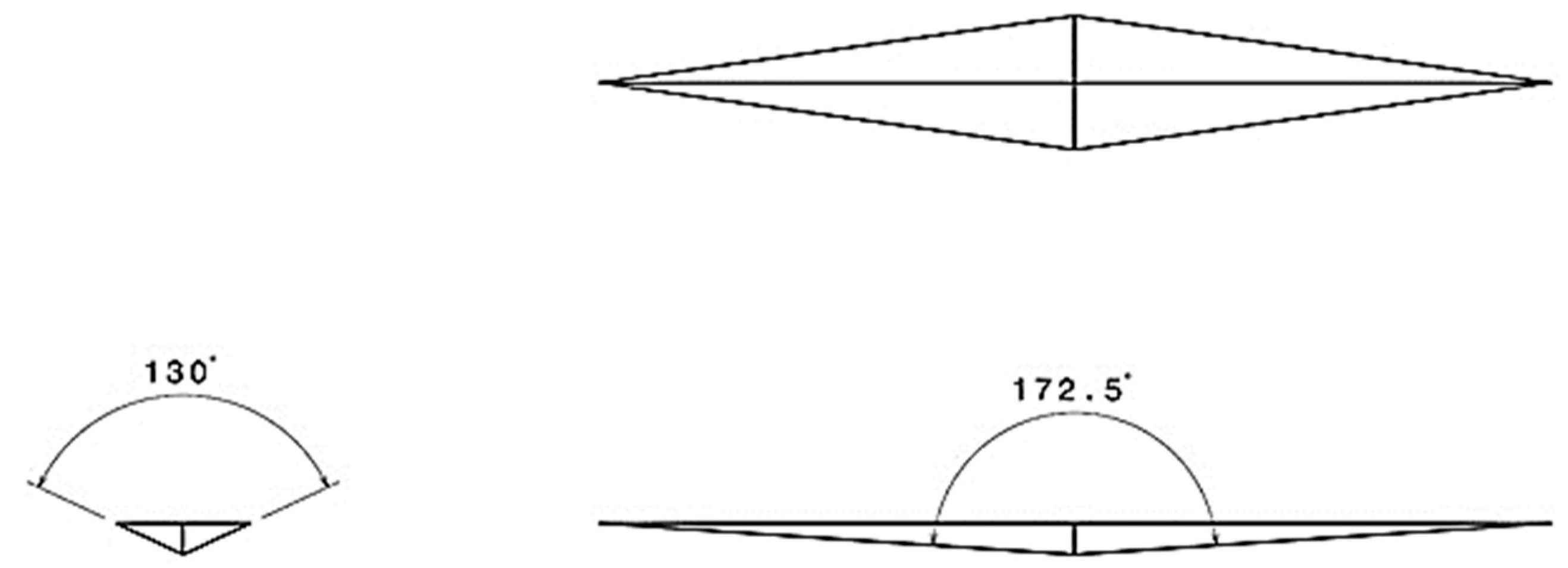
Figure 2.
Knoop indenter modeled with Bezier surfaces: (a) general view; (b) detail of the indenter tip imperfection.
Figure 2.
Knoop indenter modeled with Bezier surfaces: (a) general view; (b) detail of the indenter tip imperfection.
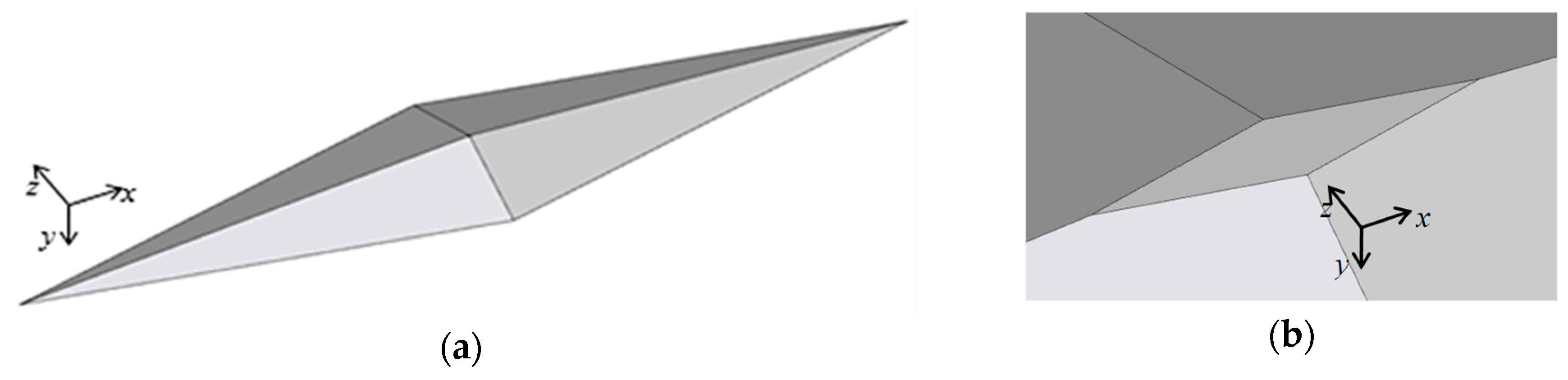
Figure 3.
Evolution of the tangents of and as function of the R-ratio values.
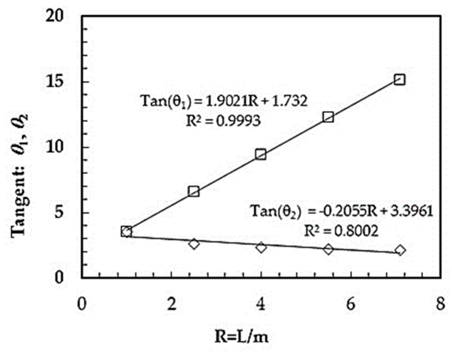
Figure 4.
Finite element mesh used in the numerical simulations: (a) global view; (b) detail of the central region where indentation occurs.
Figure 4.
Finite element mesh used in the numerical simulations: (a) global view; (b) detail of the central region where indentation occurs.

Figure 5.
Surface indentation profiles obtained along the two diagonals, the shorter, m (z-axis) and the longer, L (x-axis), respectively: (a,c) obtained at maximum load; (b,d) after unloading.
Figure 5.
Surface indentation profiles obtained along the two diagonals, the shorter, m (z-axis) and the longer, L (x-axis), respectively: (a,c) obtained at maximum load; (b,d) after unloading.

Figure 6.
Surface indentation profiles at maximum load, obtained from the results of Figure 5a,c, where z is multiplied by R = 7.11, in order to easily compare the profiles along the two diagonals, the longer, L, and the shorter, m: (a) Material M1; (b) Material 2; (c) Material M3.
Figure 6.
Surface indentation profiles at maximum load, obtained from the results of Figure 5a,c, where z is multiplied by R = 7.11, in order to easily compare the profiles along the two diagonals, the longer, L, and the shorter, m: (a) Material M1; (b) Material 2; (c) Material M3.

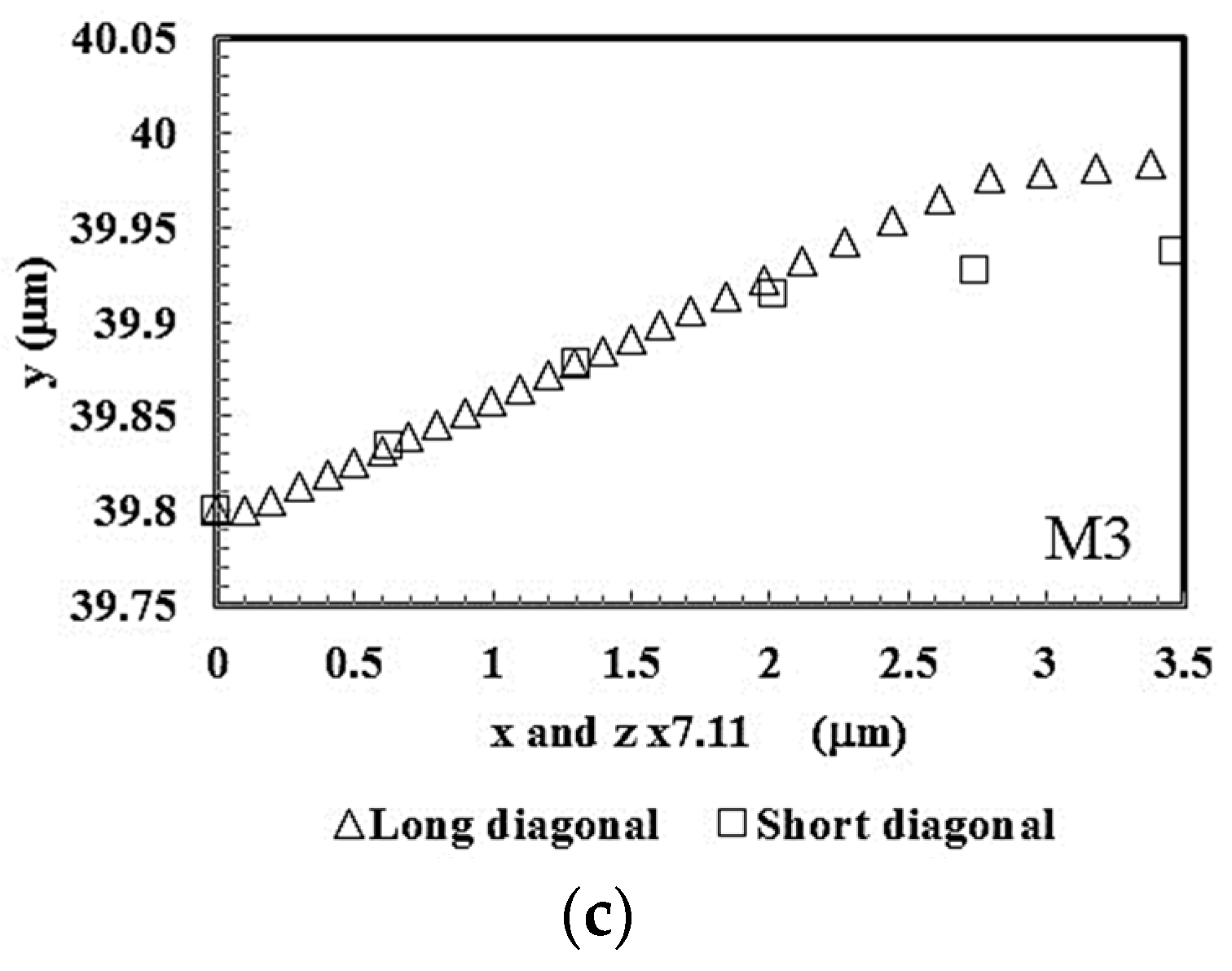
Figure 7.
Equivalent plastic strain distributions obtained at maximum load in the numerical simulations using the Knoop and Vickers indenters: (a,b) Material M1; (c,d) Material M3.
Figure 7.
Equivalent plastic strain distributions obtained at maximum load in the numerical simulations using the Knoop and Vickers indenters: (a,b) Material M1; (c,d) Material M3.

Figure 8.
Normalized contact area results obtained in the numerical simulation of the materials with the values of the strain hardening parameter, yield stress and Young’s modulus shown in Table 2, using the Knoop indenter. (a) Contact area ; (b) Contact area .
Figure 8.
Normalized contact area results obtained in the numerical simulation of the materials with the values of the strain hardening parameter, yield stress and Young’s modulus shown in Table 2, using the Knoop indenter. (a) Contact area ; (b) Contact area .
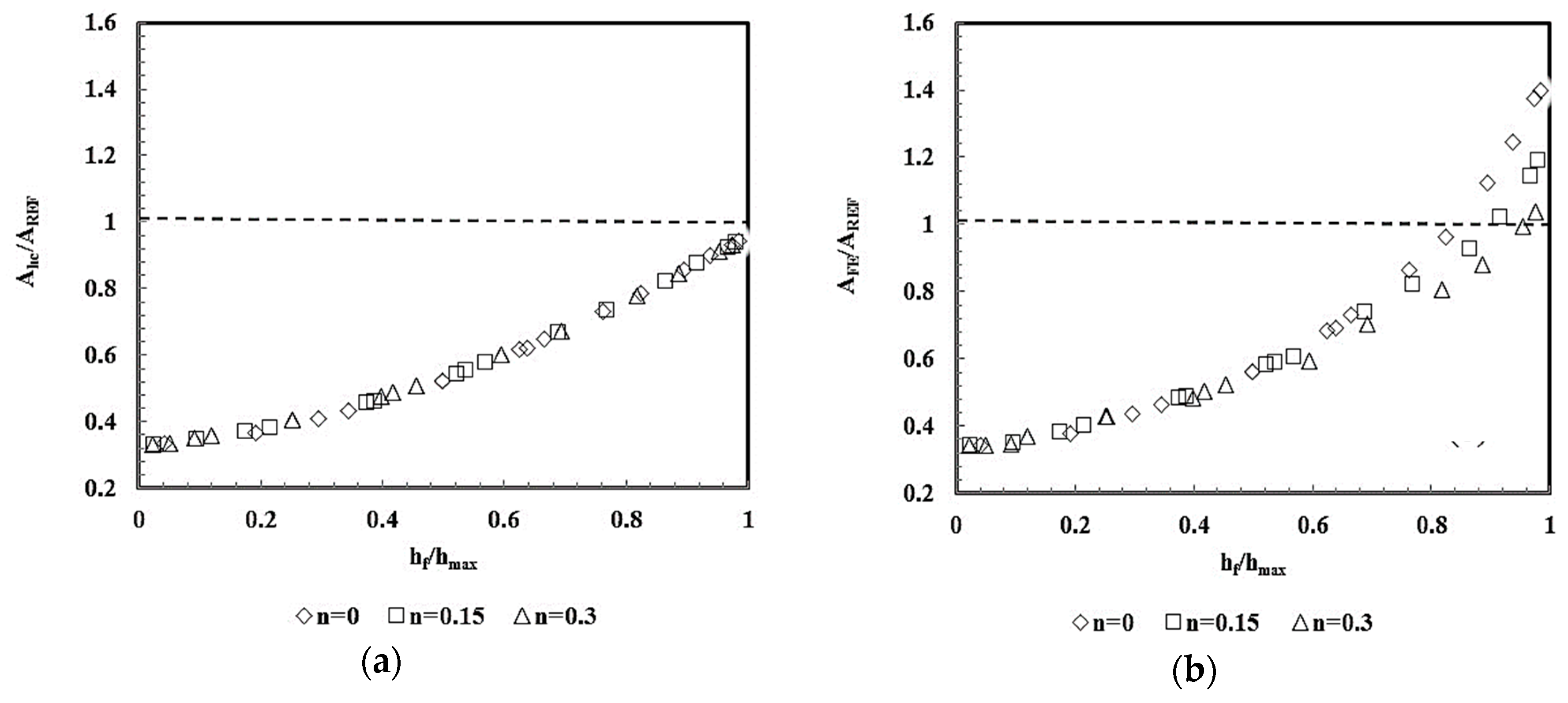
Figure 9.
Normalized Young’s modulus results obtained in the numerical simulation of the materials with the values of the strain hardening parameter, yield stress and Young’s modulus shown in Table 2, using the Knoop indenter: (a) Young’s modulus ; (b) Young’s modulus .
Figure 9.
Normalized Young’s modulus results obtained in the numerical simulation of the materials with the values of the strain hardening parameter, yield stress and Young’s modulus shown in Table 2, using the Knoop indenter: (a) Young’s modulus ; (b) Young’s modulus .

Figure 10.
Evolution of the ratio as a function of , obtained in the numerical simulations of all materials in Table 2, using the Knoop and Vickers indenters.
Figure 10.
Evolution of the ratio as a function of , obtained in the numerical simulations of all materials in Table 2, using the Knoop and Vickers indenters.

Figure 11.
Evolution of load as a function of the elastic indentation depth obtained in the numerical simulations using flat indenters with different ratio R: (a) R = 1; (b) R = 4; (c) R = 7.11.
Figure 11.
Evolution of load as a function of the elastic indentation depth obtained in the numerical simulations using flat indenters with different ratio R: (a) R = 1; (b) R = 4; (c) R = 7.11.

Figure 12.
Evolution of as a function of the R-ratio obtained in numerical simulations using the five flat and pyramidal indenters with different values of the R-ratio.
Figure 12.
Evolution of as a function of the R-ratio obtained in numerical simulations using the five flat and pyramidal indenters with different values of the R-ratio.

Table 1.
Area function of the indenters used in the numerical simulations.
| R = L/m | θ1 | θ2 | Area Function |
|---|---|---|---|
| 1 (Vickers) | 74.0546 | 74.0546 | |
| 2.5 | 69.1723 | 81.3478 | |
| 4 | 67.0462 | 83.9559 | |
| 5.5 | 65.8369 | 85.3366 | |
| 7.11 (Knoop) | 64.8379 | 86.2199 |
Table 2.
Mechanical properties of the materials used in the numerical simulations.
| Materials | Studied Cases | n | (GPa) | E (GPa) |
|---|---|---|---|---|
| Without strain hardening | 5 | ≈0 | 0.2, 2, 6, 10 and 20 | 70 |
| 5 | 200 | |||
| 5 | 400 | |||
| With strain hardening | 5 | 0.15 | 70 | |
| 5 | 200 | |||
| 5 | 400 | |||
| 5 | 0.30 | 70 | ||
| 5 | 200 | |||
| 5 | 400 |
Table 3.
Mechanical Properties of The Materials Used in the Study of The Knoop Indentation Geometry.
Table 3.
Mechanical Properties of The Materials Used in the Study of The Knoop Indentation Geometry.
| Material | (GPa) | n | E (GPa) | ν | |
|---|---|---|---|---|---|
| M1 | 0.2 | 0.01 | 200 | 0.3 | 0.97 |
| M2 | 6 | 0.3 | 0.40 | ||
| M3 | 20 | 400 | 0.25 |
Table 4.
Values obtained for the correction factor in the numerical simulations with flat indenters.
Table 4.
Values obtained for the correction factor in the numerical simulations with flat indenters.
| R = L/m | E (GPa) | Average Values of | ||||
|---|---|---|---|---|---|---|
| 30 | 200 | 400 | 600 | 800 | ||
| 1.00 | 1.055 | 1.054 | 1.053 | 1.054 | 1.054 | 1.054 |
| 2.50 | 1.125 | 1.123 | 1.124 | 1.125 | 1.124 | 1.124 |
| 4.00 | 1.215 | 1.214 | 1.214 | 1.214 | 1.215 | 1.214 |
| 5.50 | 1.269 | 1.266 | 1.267 | 1.267 | 1.266 | 1.267 |
| 7.11 | 1.374 | 1.372 | 1.371 | 1.371 | 1.372 | 1.372 |
Table 5.
Experimental Young’s modulus results.
| Materials | (GPa) [19] | (GPa) [19] | Error (%) | (GPa) [19] | Error (%) | [19] | (GPa) | Error (%) |
|---|---|---|---|---|---|---|---|---|
| Si3N4 | 317 ± 4 | 316.5 ± 4.24 | −0.16 | 300 ± 20.0 | −5.36 | 2.548 ± 0.029 | 302.8 ± 4.40 | −4.48 |
| Ceramic-glass | 82 ± 2 | 85.0 ± 0.36 | 3.66 | 85 ± 4.0 | 3.66 | 7.930 ± 0.031 | 82.1 ± 0.35 | 0.15 |
| Alumina | 385 ± 6 | 386.0 ± 7.75 | 0.26 | 380 ± 18.5 | −1.30 | 2.233 ± 0.032 | 359.4 ± 6.90 | −6.64 |
| -TCP | 130 ± 2 | 129.0 ± 0.85 | −0.77 | 142 ± 14.0 | 9.23 | 5.568 ± 0.032 | 120.7 ± 0.70 | −7.12 |
| Fused silica | 68 ± 1 | 65.0 ± 0.30 | −3.00 | 70 ± 4.0 | 2.94 | 9.221 ± 0.034 | 69.9 ± 0.25 | 2.80 |
| Average of the absolute value of the error | 1.57 | 4.50 | 4.27 | |||||
© 2018 by the authors. Licensee MDPI, Basel, Switzerland. This article is an open access article distributed under the terms and conditions of the Creative Commons Attribution (CC BY) license (http://creativecommons.org/licenses/by/4.0/).
Share and Cite
MDPI and ACS Style
Simões, M.I.; Antunes, J.M.; Fernandes, J.V.; Sakharova, N.A. Numerical Simulation of the Depth-Sensing Indentation Test with Knoop Indenter. Metals 2018, 8, 885. https://doi.org/10.3390/met8110885
AMA Style
Simões MI, Antunes JM, Fernandes JV, Sakharova NA. Numerical Simulation of the Depth-Sensing Indentation Test with Knoop Indenter. Metals. 2018; 8(11):885. https://doi.org/10.3390/met8110885
Chicago/Turabian StyleSimões, Maria I., Jorge M. Antunes, José V. Fernandes, and Nataliya A. Sakharova. 2018. "Numerical Simulation of the Depth-Sensing Indentation Test with Knoop Indenter" Metals 8, no. 11: 885. https://doi.org/10.3390/met8110885
Note that from the first issue of 2016, this journal uses article numbers instead of page numbers. See further details here.