An Analysis of Electroplated cBN Grinding Wheel Wear and Conditioning during Creep Feed Grinding of Aeronautical Alloys


1
Department of Mechanical Engineering, University of the Basque Country, Plaza Torres Quevedo 1, 48013 Bilbao, Spain
2
Industria de Turbo Propulsores S.A., Parque Tecnológico Edificio 300, 48170 Zamudio, Spain
3
University of Valenciennes, CNRS, LAMIH UMR 8201, F-59313 Valenciennes, France
*
Author to whom correspondence should be addressed.
Metals 2018, 8(5), 350; https://doi.org/10.3390/met8050350
Submission received: 9 April 2018
/
Revised: 8 May 2018
/
Accepted: 9 May 2018
/
Published: 14 May 2018
(This article belongs to the Special Issue Machining and Finishing of Nickel and Titanium Alloys)
Abstract
:Cubic boron nitride (cBN), in addition to diamond, is one of the two superabrasives most commonly used for grinding hard materials such as ceramics or difficult-to-cut metal alloys such as nickel-based aeronautical alloys. In the manufacturing process of turbine parts, electroplated cBN wheels are commonly used under creep feed grinding (CFG) conditions for enhancing productivity. This type of wheel is used because of its chemical stability and high thermal conductivity in comparison with diamond, as it maintains its shape longer. However, these wheels only have one abrasive layer, for which wear may lead to vibration and thermal problems. The effect of wear can be partially solved through conditioning the wheel surface. Silicon carbide (SiC) stick conditioning is commonly used in the industry due to its simplicity and good results. Nevertheless, little work has been done on the understanding of this conditioning process for electroplated cBN wheels in terms of wheel topography and later wheel performance during CFG. This work is focused, firstly, on detecting the main wear type and proposing a manner for its measurement and, secondly, on analyzing the effect of the conditioning process in terms of topographical changes and power consumption during grinding before and after conditioning.
1. Introduction
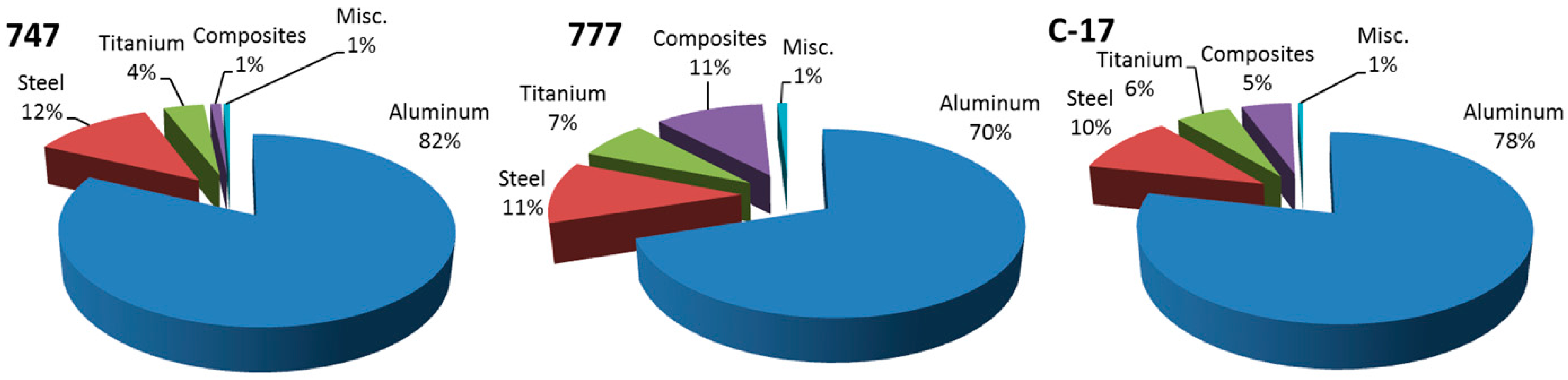
Aircraft are formed by numerous parts made of a wide variety of materials, depending on their applications. On the one hand, the outer structure is mainly made of materials with a good ratio of strength to weight, for example aluminum alloys and composites, while steel and titanium alloys are used as well to a lesser extent as compared to turbines [1] (see Figure 1). On the other hand, the turbine components are made of special titanium alloys and nickel alloys, which are called superalloys [2]. These materials are also called high-performance alloys due to their excellent mechanical strength, resistance to thermal creep deformation, good surface stability, and resistance to corrosion.
As a consequence of these enhanced properties, the manufacturing processes of the parts made of these materials need to be carried out either under special conditions or with special tools. Furthermore, the components of the engines tend to have complex geometries, which hamper the process in terms of the clamping systems and machining paths.
One of these parts is the nozzle guide vane (NGV). The different stages of the turbine stator are formed by NGVs of different sizes. Its composition together with a front and a rear view of its geometry can be seen in Figure 2. This workpiece is firstly cast by lost wax casting. The excess material left by this process, commonly above 1 mm, is removed by subsequent grinding operations until the workpiece is within the form and dimensional tolerances. While the amount of material to be removed points to milling as a more productive process, the properties of this material require the use of tougher tools such as grinding wheels.
Grinding has typically provided low material removal rates, and as such is not suitable for the increased productivity requirements of the aeronautic industry. As an alternative, creep feed grinding (CFG) conditions are used for grinding these workpieces instead of conventional grinding conditions.
A grinding process is classified as creep feed grinding when the cutting depth is larger than the grain protrusion height of the wheel [3]. Compared with a conventional grinding operation, in CFG, the cutting depth is usually above 0.5 mm. The cutting speed also increases up to 120 m/s and the feed rate decreases to values below 240 mm/min. As a result, the material is removed in one or very few strokes, diminishing the machining time.
As counterpoints, the contact length increases, the chip becomes thinner and longer, and the number of contacting grains that rub and plow the material increases to the detriment of the actual cutting grains. As a result, the thermal stress, as well as the forces in the contact zone, increase. The choice of the right grinding wheel is important for minimizing the adverse effects mentioned previously in order to manufacture these expensive workpieces without defects.
Dressable wheels are widely used in CFG using continuous dressing with the purpose of having the wheel within the desired conditions of porosity, grain sharpness, and grain protrusion height [4]. However, this method entails high radial wear, which is an inconvenience when the grinding operations do not involve straight surface grinding. Among all the surfaces to be ground in an NGV, some of them require a specific path to be followed by the wheel, which at the same time depends on the workpiece and the wheel geometry. If the radial size of the wheel varies significantly, not only should the path to be followed and the grinding parameters be adapted continuously, but also the position of the nozzles required for the high-pressure cooling system. As has been mentioned before, productivity is becoming more and more important in this sector. Hence, non-dressable grinding wheels, such as electroplated wheels, are being used, especially when the grinding is not a straight surface grinding operation.
These wheels are formed by three components, namely, a steel hub, a nickel layer acting as the bonding material, and abrasive grains. Knowing the manufacturing process of these tools is necessary to understand its qualities, and therefore, it is explained as follows [5]. First of all, the steel hub is given nearly the final form of the wheel, and the only difference as compared to a finished wheel should be the offset for the bond and grains. Later, the hub can be heat-treated and the working surface of the wheel is completely covered by abrasive grains. Then, the electroplating process is carried out in two steps by an electrolytic bath where the wheel (the cathode) is soaked in a watery solution of metal salts such as Ni, Ag, Cu, Au, or Co (the anode). Firstly, it is soaked in a motionless bath where the grains are slightly covered and fixed to the hub. Secondly, the excessive grains are removed and the wheel is soaked in a circulating electrolytic bath where the desired plating layer thickness is achieved. The junction between the grains and the bond is mechanical. As a consequence, the grains must be covered up to 50% their size. In spite of the low resulting grain protrusion height, the process is carried out at a low temperature (≤60 °C) which avoids the presence of residual stresses.
In this way, the electroplated wheels have only one abrasive layer. Therefore, with the purpose of extending the wheel life for the sake of productivity and tool cost, superabrasive grains are being used rather than conventional abrasives. Cubic boron nitride (cBN) and diamond are the two superabrasives used for the grinding wheels. The latter is around two times harder than the former but it is susceptible to reacting chemically with some of the components of the C1023, namely, nickel, cobalt, tantalum, and titanium [3]. In addition, in the presence of oxygen, at temperatures above 650 °C, it is converted into graphite.
As has been explained before, one of the features of CFG is the high temperature in the contact zone due to the increase in friction. The properties of the superalloys involve per se high temperatures during the machining processes. In combination, the temperatures in the contact zone in the present case are likely to increase the threshold of 650 °C. Taking everything into account, electroplated cBN grinding wheels are used in the CFG process of C1023 NGVs.
However, since it is a non-dressable wheel, the wear state of the wheel surface changes during its lifetime. The density of active cutting grains increases as the grain protrusion height decreases, which diminishes the chip thickness. These phenomena may eventually lead to a common type of wear in grinding, called wear flat [4]. This can be defined as the appearance of flat planes parallel to the cutting velocity on the grains. In consequence, the normal force increases in order to reach the pressure needed for penetrating the material, causing, at the same time, an increase in the tangential force. By extension, there is more rubbing and plowing and, consequently, higher temperature and higher force. In some cases, these phenomena lead to the critical failure on the ground surface such as thermal damage, vibration marks, and dimensional inaccuracies.
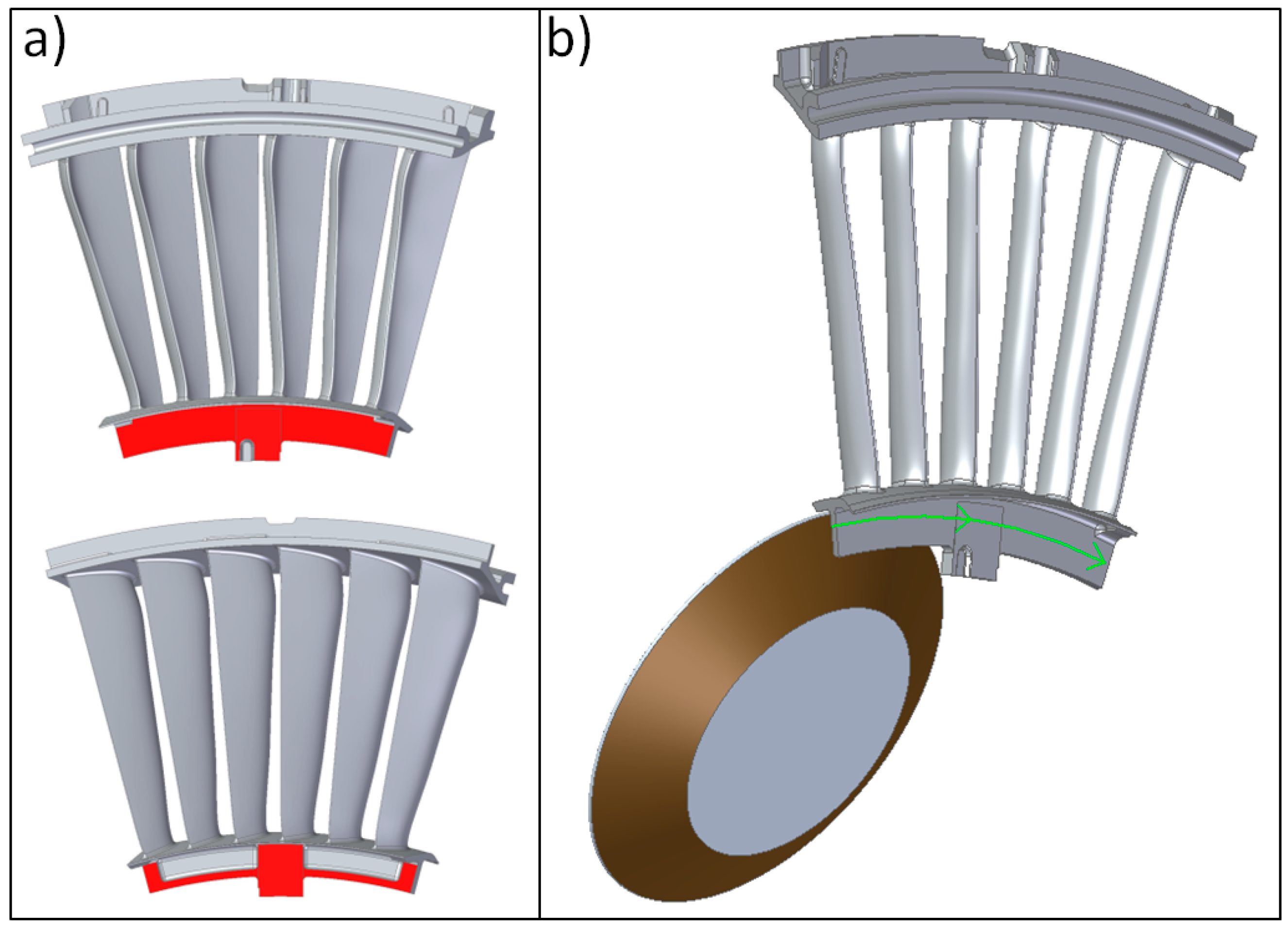
The particular features of each surface to be ground make some of them more susceptible to suffering these phenomena. This is the case of the inner rail, marked in red in Figure 3a. This surface is ground by means of a conical grinding wheel, for which the path is drawn in Figure 3b.
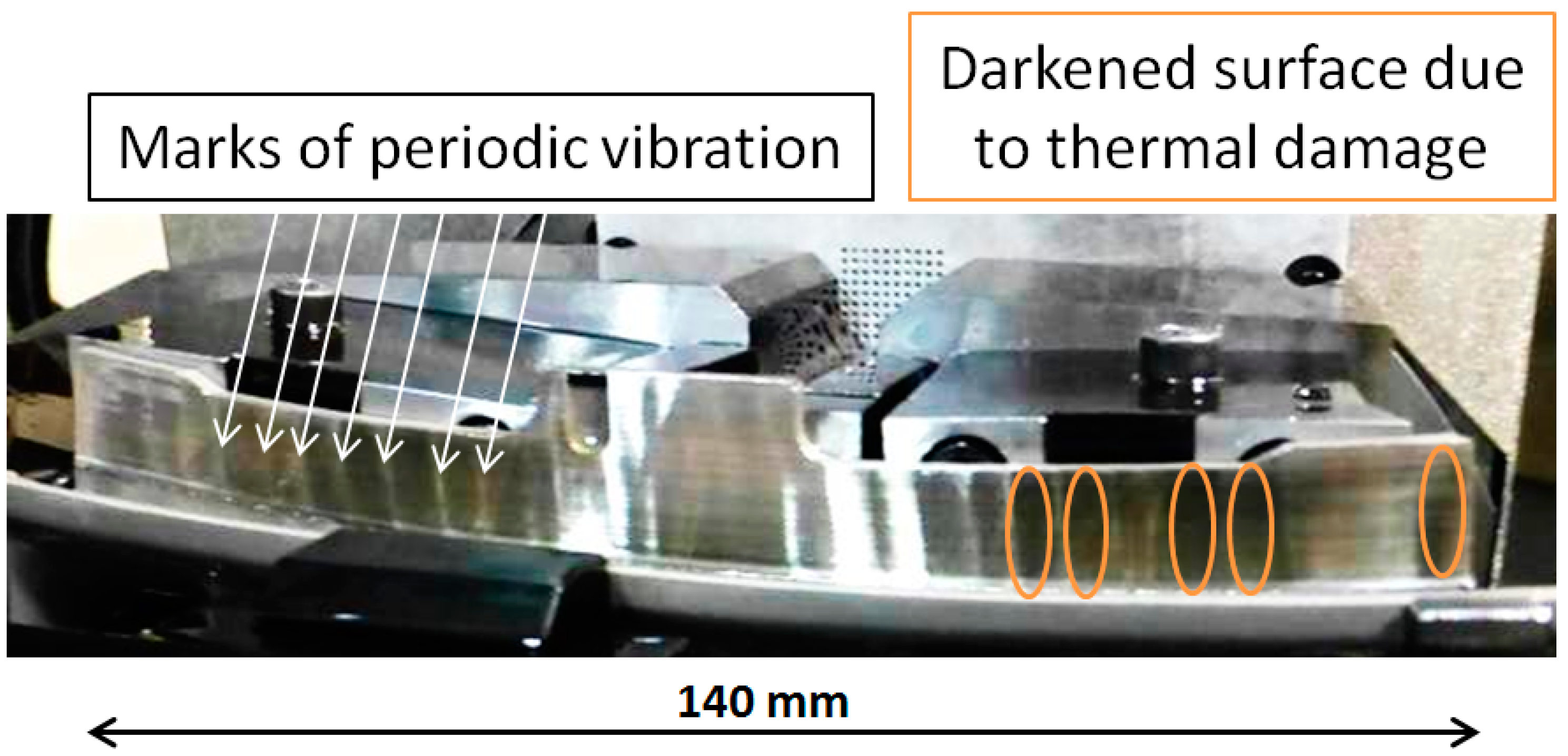
As a consequence of the grinding operation, this surface can only be supported by the opposite side instead of being rigidly clamped. Moreover, there is a low material volume for dissipating the heat generated during grinding. As a result of increasing wheel wear, this surface is likely to present the vibration marks and thermal damage mentioned previously, as shown in Figure 4.
Nevertheless, despite the fact that electroplated wheels are not dressable, their surfaces can be conditioned for partially recovering the cutting ability. Numerous methods have been developed for conditioning the wheel surface. Mechanical dressing with fixed dressing tools is a widespread method used because of its simplicity and lack of special equipment. As was explained by Wegener et al. [6], block sharpening is a method especially used for monolayer cBN wheels where a stick made of alumina or silicon carbide (SiC) in vitrified or resin bond is pressed against the grinding wheel. The contact width normally covers the whole grinding wheel width and it is applied under two different configurations. On the one hand, the constant radial velocity provides a better control of the grinding wheel topography but causes high force peaks at the beginning of the contact. On the other, the constant normal (radial) force may take more time but those force peaks are avoided, which is crucial in monolayer wheels since they can lead to grain pullout.
In this way, the wheel is sharpened and the previous problems are avoided in the subsequent workpieces. However, the real effect on the wheel needs to be studied and understood in order to know how it affects the wheel life.
In this work, an analysis of the wheel surface was carried out at different wear states with the purpose of characterizing the wear types along the wheel life and proposing some roughness parameters to quantify them. Once the wear types responsible for the vibration and thermal problems were described, the effect of the conditioning process was studied in order to understand how it modifies the wheel topography and how such modification affects the wheel performance in the long term.
1.1. State of the Art
1.1.1. Electroplated cBN Wheel Surface Characterization
Different methods have been developed for measuring the wheel topography. Some authors [7,8,9,10,11] have worked on online methods. Brinksmeier and Werner [7] obtained two dimensions (2D) roughness parameters of the wheel surface by laser beam triangulation on corundum grinding wheels. Furutani et al. [8] measured the radial wear and the dulling and loading of vitrified alumina grinding wheels by a pressure sensor. They recorded the hydrostatic pressure of a cutting fluid jet after contact with the wheel surface with a specific gap between the sensor and the wheel. Later [9], they successfully used the same setup for compensating the grinding depth in surface grinding. Acoustic emissions were used by Sutowski et al. [10] and Liao et al. [11] with the purpose of detecting a dull state of the grains.
The study presented here was carried out for the electroplated cBN grinding wheels. The workpiece was the above mentioned NGV made of C1023. This process was carried out in a five-axis grinding machine, where the kinematics required were intricate. Furthermore, depending on the geometry to grind, the simultaneous movement of the wheel and workpiece was necessary. In addition, a high amount of high-pressure oil-based cutting fluid was used through two sets of nozzles, one before the contact for lubricating the contact zone and the other after the contact for cleaning the wheel. Therefore, the previously explained methods were disregarded because of the special conditions needed for the optical, acoustic, or pressure sensors. Furthermore, some of them were focused on measuring specific phenomenon on the wheel surface instead of using standardized spatial roughness parameters gathered by the standard International Organization for the Standardization (ISO) 25178.
Concerning the offline methods, they allow having a deeper knowledge of the wheel surface. Contact measuring devices, namely, stylus profilometers, were used for characterizing the wheel surface either directly on the wheel surface or on a replica of the surface. Due to the physical nature of the stylus profilometer, the diamond tip can hardly reach the deepest valleys of the surface and in some cases, some information is lost. This is called convolution error. Blunt and Ebdon [12] used this technology with the purpose of measuring the surface of vitrified aluminum oxide grinding wheels. They carried out the measurement on the wheel surface because of the previously explained convolution error. In this way, the acquisition of the information corresponding to the grain tips was ensured. After analyzing their results, they established the optimum sample spacing for obtaining the grain density (see Equation (1)). Here, SSopt is the optimum sample spacing and dg is mean grain size.
Butler et al. [13] used the same measuring strategy and type of wheels and applied the optimum sample spacing expression as well. They studied the wheel surface after different wear states and were able to correlate the wear state with the grinding forces during the wheel life.
Optical devices have been successfully used for characterizing electroplated cBN grinding wheels. Shi and Malkin [14] used an optical microscope for determining the wear flat area, active grain density, and grain pullout on the electroplated cBN wheels in the internal cylindrical grinding of bearing steel. However, any roughness parameter of the wheel surface could not be taken and hence, the state of the grains without wear flat remained unknown. Upadhyaya and Fiecoat [15] also used optical microscopy for the grain pullout measurement in the CFG of stainless steel. Later, Guo et al. [16] found grain fracture together with grain pullout and wear flat with the same methodology in the same type of wheels during surface grinding of nickel base superalloy. However, they only quantified the wear flat area percentage disregarding the fractured grains. Ding et al. [17] went further and quantified the attritious wear, microfracture, and macrofracture in terms of percentage of all the grains by using optical and scanning electron microscopy in a CFG operation of a nickel base superalloy. Finally, Yu et al. [18] managed to measure the electroplated cBN grinding wheel surface in three dimensions (3D) with a digital microscope with the aim of achieving a grain height distribution. They used this information for a wheel life expectancy model during the nickel base superalloy grinding.
Although most of the works reviewed previously are focused on the same grinding wheels, workpiece materials, and grinding process, none of them assessed the wheel surface in terms of the roughness parameters as Butler et al. [13] and Ye et al. [19] did. The authors of the first study established Sds (summit density), Ssc (mean summit curvature), and Sq (root mean square roughness) as the most suitable parameters for the wheel wear characterization of alumina wheels in the surface grinding of steel. In the other study, Ye et al. used infinite focus measurement technology for the 3D digitalization of diamond wheels. They established Spd (number of peaks per unit area), Sha (mean hill area), and Shv (mean hill volume) parameters of the standard ISO 25178 for quantifying the wear of the grinding wheel surface.
The predominant wear types not only depend on the grinding wheel features but also on the workpiece material and grinding parameters. The electroplated cBN grinding wheel wear has not been characterized nor quantified by means of the roughness parameters during the CFG of the nickel-based superalloy. This was addressed in the first part of this work by means of offline optical methods and supporting on the standard of the ISO 25178.
1.1.2. Electroplated cBN Grinding Wheel Conditioning
Much effort has been done especially in the field of conditioning electroplated superabrasive grinding wheels, either for removing the runout or for dressing the grains. As they are monolayer wheels, they present specific features that make their conditioning process different to that of the rest of wheels. The higher hardness of the grains often requires very specific abrasive materials or methodologies if they are dressed by means of contacting dressers. However, the metallic bonding allows the use of non-conventional conditioning methods, such as laser or even methods that take advantage of the electrical properties of the metals. Moreover, in these wheels, the process must be accurately controlled, otherwise, the bonding layer can be critically damaged or the grain protrusion height excessively diminished. These faults would not be possible to be corrected by subsequent conditionings because there is only one abrasive layer. The latest works and a further explanation of each method are presented in the following lines.
Ghosh and Chattopadhyay released two consecutive works [20,21] based on touch dressing. This conditioning method was used for single layer grinding wheels in order to minimize the runout of the wheel and sharpen the grains. In this method, SiC or diamond blocks were used with a shallow depth of cut, in the range of microns, in order to touch only the grain tips. In the first work [20], they studied the influence of dressing brazed cBN wheels with different grains distribution patterns in the surface finishing and grinding forces. The dressing tool was formed by flattened diamonds brazed on a block. They concluded that after dressing the wheel surface, the resulting workpiece roughness in terms of Ra, Rz, and Rmax was similar for all the grain patterns but slightly better for the wheels with lower grain density since they offered more inter-grit chip space, Ra = 1 μm against 1.5 μm. Regarding the force values, they also verified the grain micro-fracture instead of wear flat appearance as a consequence of the process. Later they performed [21] the same study for different grain sizes with similar results. Similar surface roughness was achieved either with coarse and fine grains while the grinding performance was still better with coarser grains thanks to the separation of the grains.
Zhao and Guo [22] recently used three different wheel conditioning methods consecutively for electroplated diamond wheels in order to enhance their performance in the ultra-precision grinding of optical glasses. Firstly, they used a metal bonded diamond cup wheel with a lower grain size than the grinding wheel with two purposes: to minimize the runout and to flatten the grains to the bond layer level in order to enhance the finishing. Secondly, they proposed the electrolytic in-process dressing (ELID) method for removing a thin layer of the bonding material. In this way, a small grain protrusion height was achieved. Finally, they used an Al2O3 stick to remove the oxide layer created by the ELID process.
Kitzig et al. [23] applied ultrasonic assisted dressing (UAD) on electroplated grinding wheels. This method had been widely used for dressing vitrified and resin bonded grinding wheels but not for monolayer grinding wheels. By dressing coarse grain wheels (D251) using this method, authors achieved surfaces roughness values comparable to those obtained by fine grain wheels (D46 and D181) in spite of the drastic increase of the normal force (from 15 N to 55 N) and the force ratio (from 2 to 3.5).
Laser touch dressing (LTD) is widely used for dressing multilayer grinding wheels and it was introduced to monolayer wheels by Dold et al. [24] who used a picosecond laser source for dressing electroplated diamond wheels. They compared laser touch dressed wheels with mechanically touch dressed wheels for dressing SiC grinding wheels. They achieved lower dressing forces with the wheels that were previously touch-dressed by laser. In addition, the wear of the wheels after dressing the SiC wheel was assessed in terms of Ra and Rz and the wheels mechanically dressed showed lower values and, therefore, a better result.
Recently, Pfaff et al. [25] used LTD on electroplated cBN wheels without causing thermal damage. They compared LTD and conventional dressing in terms of the grinding forces, workpiece roughness, and wheel´s peaks bearing ratio. The forces measured after grinding 100Cr6 steel resulted in lower values for the wheel dressed conventionally due to an uneven grain protrusion height, which also led to worse surface finishing and higher wheel wear.
It should be noted that in the works cited previously, the mechanical, UAD, and non-contact methods were used for different purposes such as equalizing the grain protrusion height while keeping a rough surface on the grains, flattening the grains for a better finishing, and cleaning the bonding layer. Nevertheless, none of the works cited previously studied the wheel performance in the long term after being dressed by means of touch dressing. In this work, the wheel topography before and after the conditioning process was compared and the spatial roughness parameters were proposed in order to understand the topography change suffered by the grains. Furthermore, the effect on the grinding performance during the wheel life was assessed by means of power consumption.
2. Materials and Methods
2.1. Wheel Surface Characterization during CFG
Wheel topography analysis was carried out for two purposes. One of them was to characterize the wear during the wheel life through analyzing the wheel after different amounts of accumulated material removal, Vw, in order to achieve different wear states. The second purpose was to understand and assess the effect of the conditioning by means of analyzing the wheel before and after such processes.
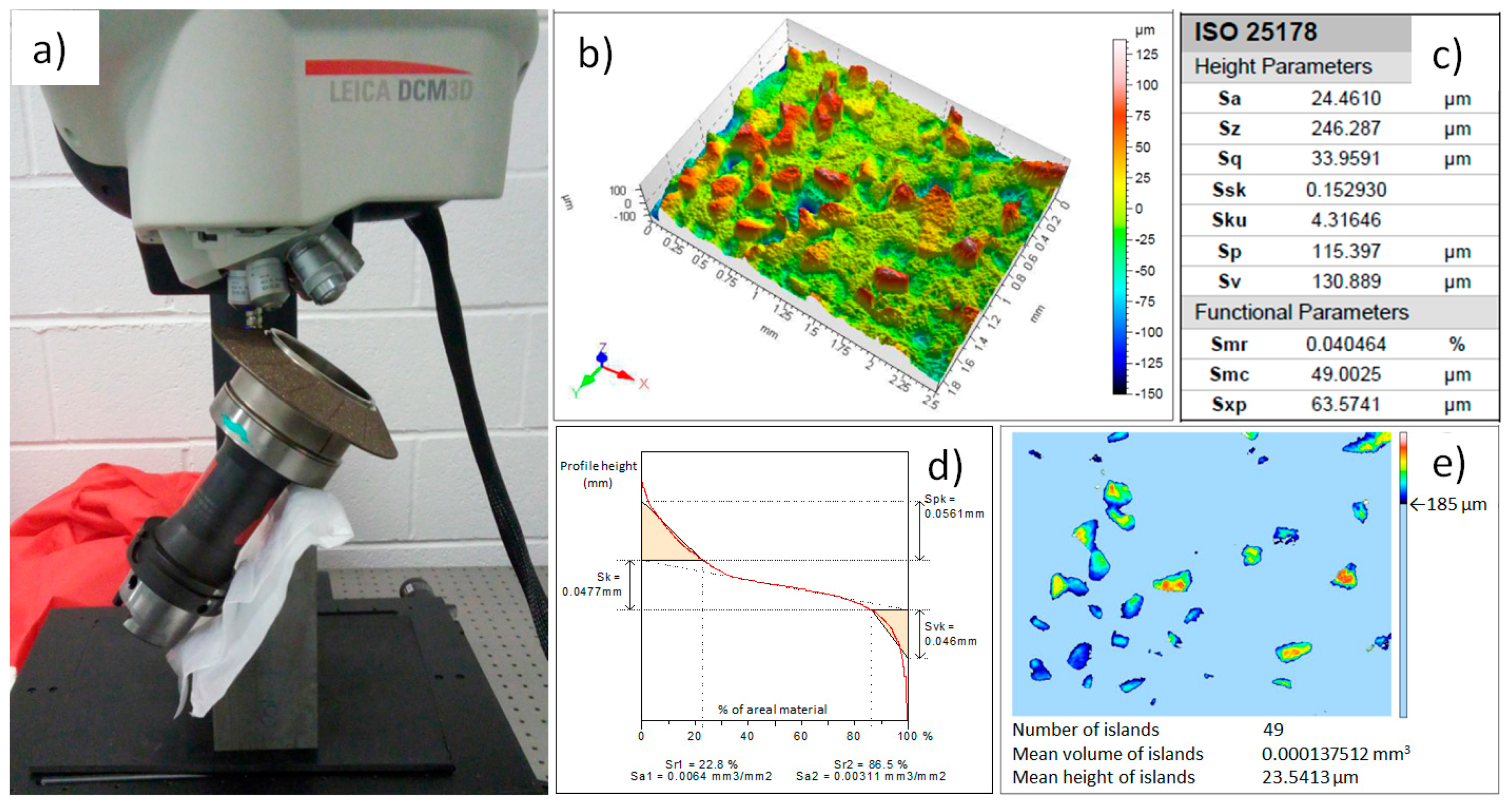
The characterization was carried out offline using optical devices. A confocal microscope Leica DCM 3D® (Leica microsystems AG, Wetzlar, Germany) with 5× magnification was used for digitalizing the wheel surface, thus quantitatively characterizing the wheel wear. Later, the Leicamap® (Leica microsystems AG, Wetzlar, Germany), and Talymap® (Taylor Hobson, Leicester, UK) commercial software were used for obtaining 3D spatial roughness parameters as well as Abbott–Firestone curves and other diagrams. Some of them are shown in Figure 5. Each wheel was characterized in six different zones along the circumference. These zones were equally spaced one from each other in order to obtain mean values representative of the whole state of the wheel.
In contrast, the Leica DSM 300® (Leica microsystems AG, Wetzlar, Germany) macroscope was used for taking real pictures of the wheel surface. These images were used as complementary information for the digitalization. Thanks to these pictures, the actual state of the wheel surface was observed and different phenomena as the presence of stuck material could be assessed. In some cases and for complementary information as well, the scanning electron microscope (SEM) Jeol 6400® (Jeol Ltd., Tokyo, Japan) was used.
2.2. Roughness Parameters Analysis
There are numerous roughness parameters within the ISO 25178 standard. Each of them is properly defined and its application depends on the phenomena that should be analyzed. Apart from these parameters, other numerical values can be drawn from the digitalization with the analysis software, as was explained in the previous section. In this paper, given such a number of parameters and with the purpose of choosing the most representative ones for measuring the wear types, the authors used a statistical method called the average and standard deviation method. The following lines introduce that method, which is more widely explained in the book written by Leach [26].
It should be noted that this method is suitable for differentiating between two states (classes) of the sample. For a multi-class case, other mathematical methods should be chosen.
Given two different wear states of grinding wheels with the same specifications, non-used (N) and completely worn (W), it is important to know which parameter or parameter combination is the most appropriate for distinguishing both states numerically.
The first step is to create the feature vector for each sample. The feature vector comprises all the different parameters of a sample n, from s1 to sm, as depicted in Equations (2)–(4).
Then, every si parameters of the same class must be gathered together. In this way, two vectors of parameters are resultant for every si parameter, one for each class. The vectors of the example are gathered in Equation (5).
For each of the vector, the mean values and standard deviation are calculated using the expressions of Equations (6) and (7), respectively.
In the next step, the intervals for new wheels and worn wheels are calculated using the coverage factor k by means of Equation (8).
The value of k represents the level of confidence of the normal distribution curve according to the probability density function and corresponds with the percentage of the samples of each class covered by the curve. In this work, the following values for k were used.
- k = 1: Corresponds to 68%.
- k = 2: Corresponds to 95%.
- k = 3: Corresponds to 99.7%.
The two resulting normal distributions can be completely separated or not. If there is overlap among them, there is a band of values of the parameter where the wheel can be classified as new and as worn at the same time and hence, lead to unclear conclusions. Therefore, a parameter can be considered suitable for classifying the wheels if the normal distribution curves are disjunct.
Nevertheless, the parameters that present the disjunct distributions present different suitability levels for the classification of the wear state of the wheel as well. The suitability of the parameters is called significance and it is calculated through Equation (9). There, is the difference between the lowest point of the highest interval and highest point of the lowest interval and it is divided by the mean point between the two average values.
A high Si means that the parameter can be considered as representative of the wheel wear, whereas a negative Si indicates that the normal distribution curves overlap. As a conclusion, the parameter with the highest Si must be selected as the most representative of the wheel wear. However, it should be noted that Si depends not only on the distance between the average values but also on the standard deviation due to the coverage factor. In this way, a parameter with a high standard deviation may have the highest Si under a low coverage factor if its averages are the most distant, but it may result in negative Si when a high confidence level is applied.
Once the most significant parameters are achieved, the threshold τ that discriminates between the new and the worn wheel must be calculated. If there is overlap between the intervals, the threshold matches with the intersection point of the two Gaussian distributions. The threshold can be found from Equation (10).
In the same work, the authors also proposed an alternative method for a two-class case. It is called the correlation coefficient method and was described as less robust. In this method, Equation (11) must be used for calculating the so-called correlation coefficient:
where si is the parameter that is being assessed, μ is the mean value of that parameter, and n refers to the number of samples. If the resulting rGB is close to one, the corresponding parameter can be used as a classifier. If it is close to zero, another parameter must be used for that purpose.
In this paper, the average and standard deviation method was applied in the first place because of its connection to the basis of statistics. The correlation coefficient was considered as a substitute method to use in the case of having an invalid result with the average and standard deviation method.
2.3. Wheel Conditioning
Regarding the classification of the conditioning processes made by Wegener et al. [6], the mechanical conditioning with fixed tools, namely, the SiC stick, was employed for recovering the cutting ability. The lack of need for specific equipment was the main reason why this method was used. The conditioning was carried out after the thermal and dimensional problems cited previously. The effect of the conditioning was evaluated in terms of the wheel topography and power consumption under different grinding parameters.
With the purpose of assessing the effect of the conditioning process, four different CFG operations were planned, each one with a different equivalent chip thickness (heq) (see Equation (12)).
The equivalent chip thickness is a parameter commonly used for classifying grinding operations, where ae is the cutting depth, vw is the feed speed, and vs is the cutting speed. Table 1 shows the gathered details of this study. Test1 and Test2 are roughing operations while Test3 and Test4 are semi-finishing operations. They were carried out consecutively from Test1 to Test 4 and the process was repeated until the problems in the workpiece appeared again. Then, the grinding wheel was characterized before and after being dressed. During every test, the power consumption was measured. The evolution of the power during the wheel life was considered as an indicator of the efficiency of the conditioning on the CFG process. Furthermore, using different heq, the sensitivity of different CFG operations to the conditioning can be evaluated.
3. Results
3.1. Wheel Wear Analysis
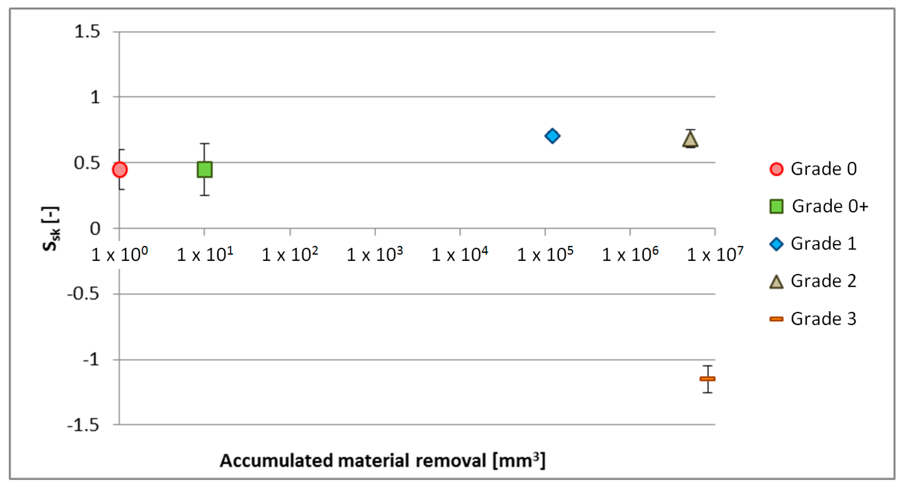
The wheel was observed after five different wear states, namely, a brand new wheel (grade 0), after being dressed with a SiC stick (grade 0+), after grinding 122 cm3 (grade 1), after grinding 5070 cm3 (grade 2), and after grinding 8112 cm3 (grade 3). The volume of the material removed in the last state corresponds with the end of the wheel life according to industrial experience.
3.1.1. Qualitative Analysis
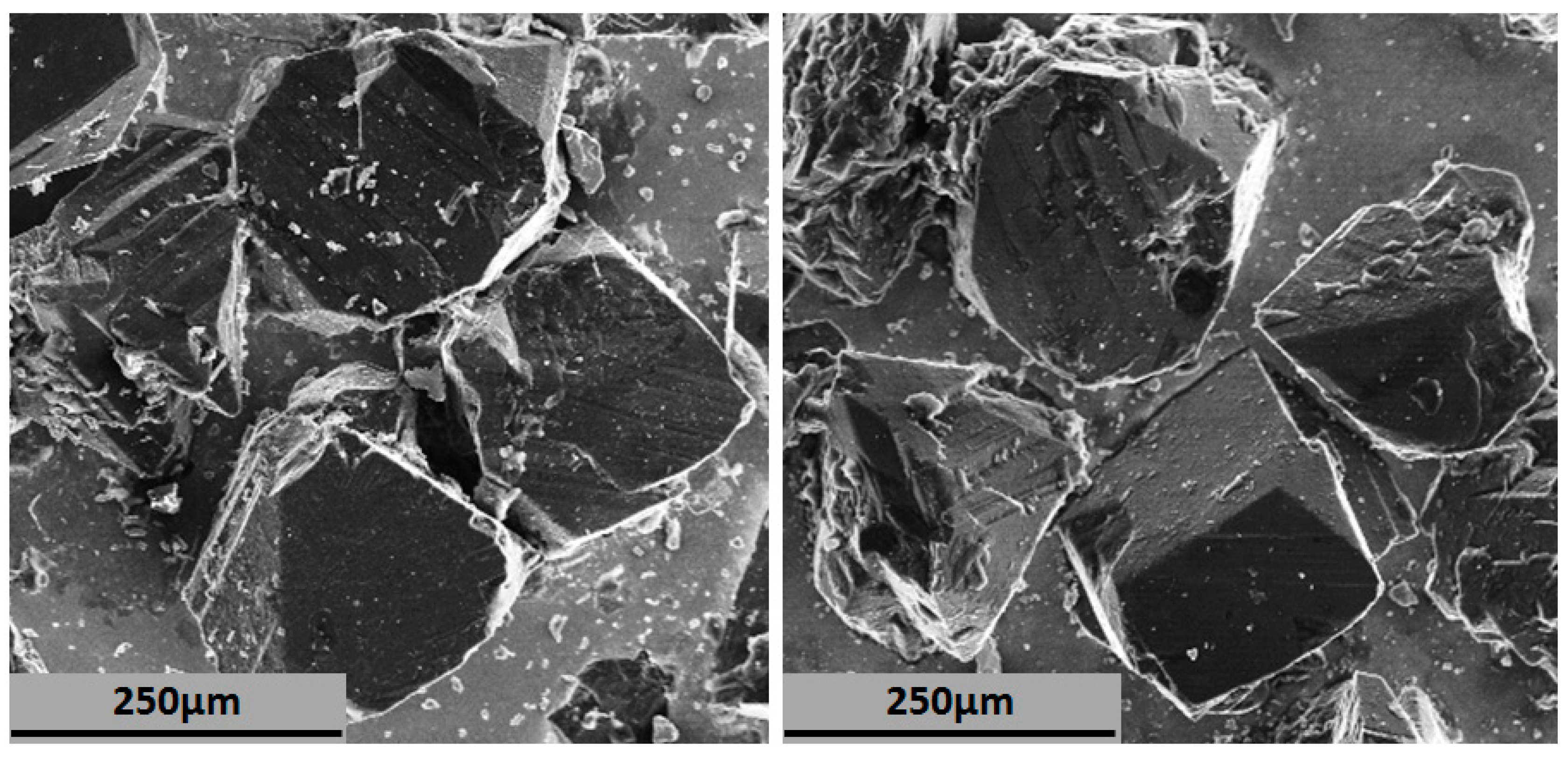
Firstly, the wear types were detected using optical pictures. Figure 6a,c show a comparison of the wheel in grade 0 and Figure 6b,d show a comparison of the wheel in grade 3. The presence of wear flats was detected all along the surface while other wear types such as grain pullout and wheel loading were not found. The orange circles indicate some examples of wear flats. It should be mentioned that the flat surfaces were also found on grains belonging to the new grain surface, although they were not parallel to the vs (see Figure 6g). However, with a higher magnification, the difference between them can be clearly seen. The flat grains on a new wheel present a mirror-like surface, as shown in Figure 6e,g, while the flat grains on a worn wheel present a rough surface as consequence of the interaction with the workpiece, as shown in Figure 6f,h.
Hence, it can be concluded that wear flat is the main wear type and is responsible for the problems appearing in this process.
3.1.2. Quantitative Analysis
Once the wear types were detected, the spatial roughness parameters of the standard ISO 25178 were chosen. Since there is a high number of parameters comprised of the standard, with the purpose of optimizing the efforts, the height parameters and the functional parameters were chosen. These two groups of parameters are the most used for spatial roughness analyses and are explained in the following lines:
Height parameters:
- Sa.
- This parameter is called the Average Roughness. It provides an overall measure of the surface.
- Sq.
- This parameter is called the Root Mean Square roughness and it is equivalent to the standard deviation of heights.
- Sp.
- This is the Maximum Peak Height above the mean line.
- Sz.
- This is the Maximum Height of the surface.
- Sv.
- This is called Maximum Valley Depth below the mean line.
- Ssk.
- This parameter is called Skewness and it is a measure of the symmetry of the profile. A profile where peaks are more predominant than valleys would present a positive Ssk value, while a surface with predominantly valleys would have a negative value.
Sa and Sq are widely used in the industry for evaluating, in a rapid and easy manner, the finishing of parts manufactured under comparable procedures; Sp, Sz, and Sv provide information of the upper and lower limits of the profile; and finally, Ssk gives a sense of the distribution of the material along the height of the profile.
Functional parameters:
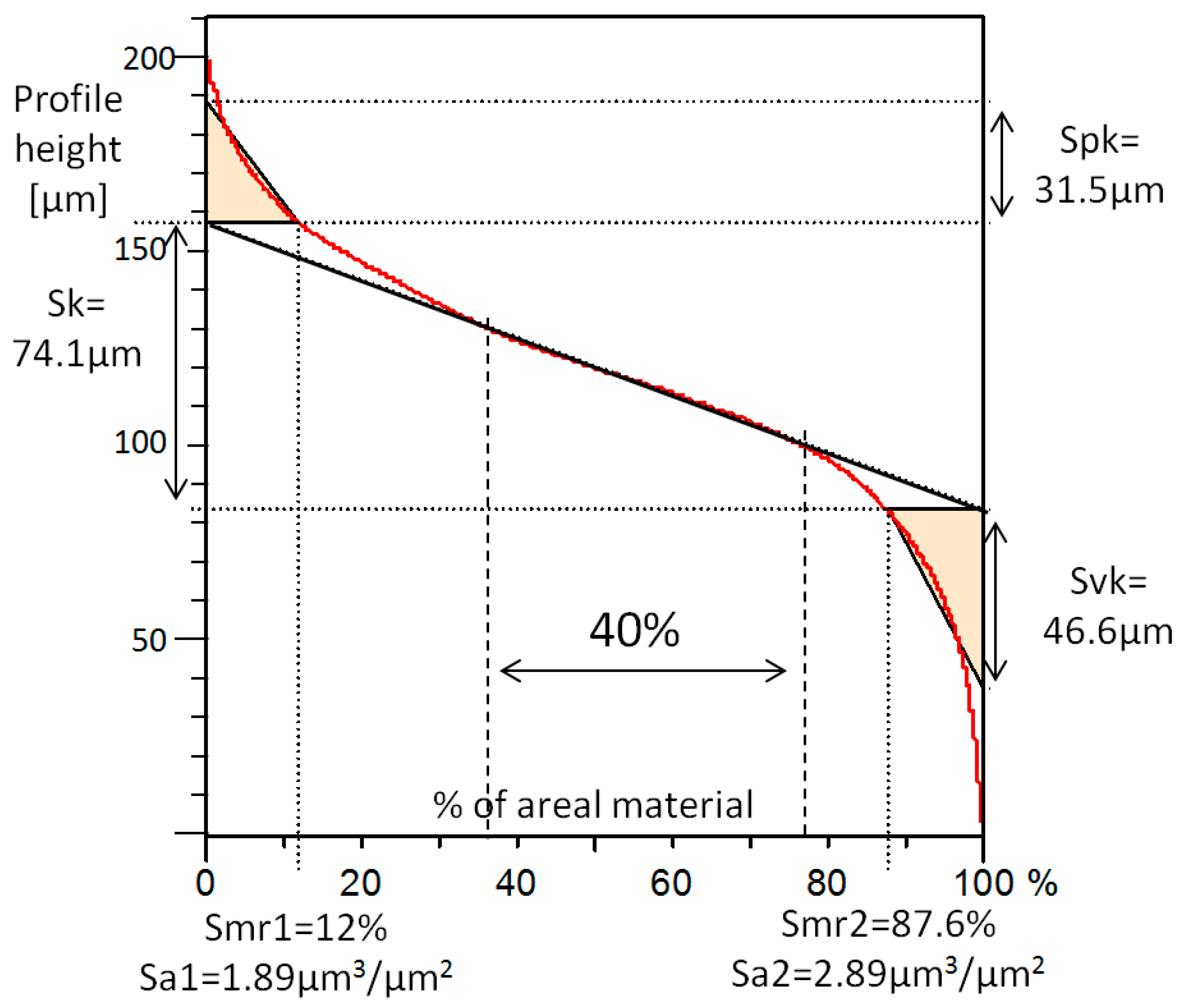
- Spk.
- The Reduced Peak Height, calculated from the Abbott–Firestone curve. This is the height of the triangle drawn above Sk in Figure 7. The area of the triangle is the same as the area covered by the red curve above the upper limit of Sk. Taking into account that the base of the triangle is the Smr1, the height of the triangle is adjusted in order to have the same area in both.
- Sk.
- The Core Roughness, calculated through the equivalent straight line. According to the ISO 25178 standard, the equivalent straight line is the one with the lowest slope that cuts the Abbott–Firestone curve in two points, distancing each other by 40% of the material. If there is more than one line with the same minimum slope, the equivalent line closer to 0% of the material, that is, the left vertical axis, must be chosen. See an example in Figure 7.
- Svk.
- The Reduced Valley Depth, calculated in a similar way to Spk. In this case, the height of the triangle must be adjusted for obtaining the same area as the area left between the red curve and the lowest limit of the Sk.
- Smr1.
- The Peak Material Portion, indicating the percentage of the areal material at the upper limit of Sk.
- Smr2.
- The Valley Material Portion, indicating the percentage of the areal material at the lower limit of Sk.
- Sa1.
- The Upper Area [27]. This is the area of the triangle formed by Spk and Sr1. The physical meaning of this parameter is the volume of material per unit of material surface above Sk.
- Sa2.
- The Lower Area. This is the area of the triangle formed by Svk and Sr2. Similar to Sa1, the physical meaning of this parameter is the volume of void space per unit of void surface below Sk.
All the functional parameters and their correspondence with the Abbott–Firestone curve can be seen in Figure 7. Spk, Smr1, and Sa1 provide information about the material distribution in the upper part of the profile; Svk, Smr2, and Sa2 provide information about the voids of the lower part; and, finally, Sk is influenced by the overall distribution of the material along the profile height.
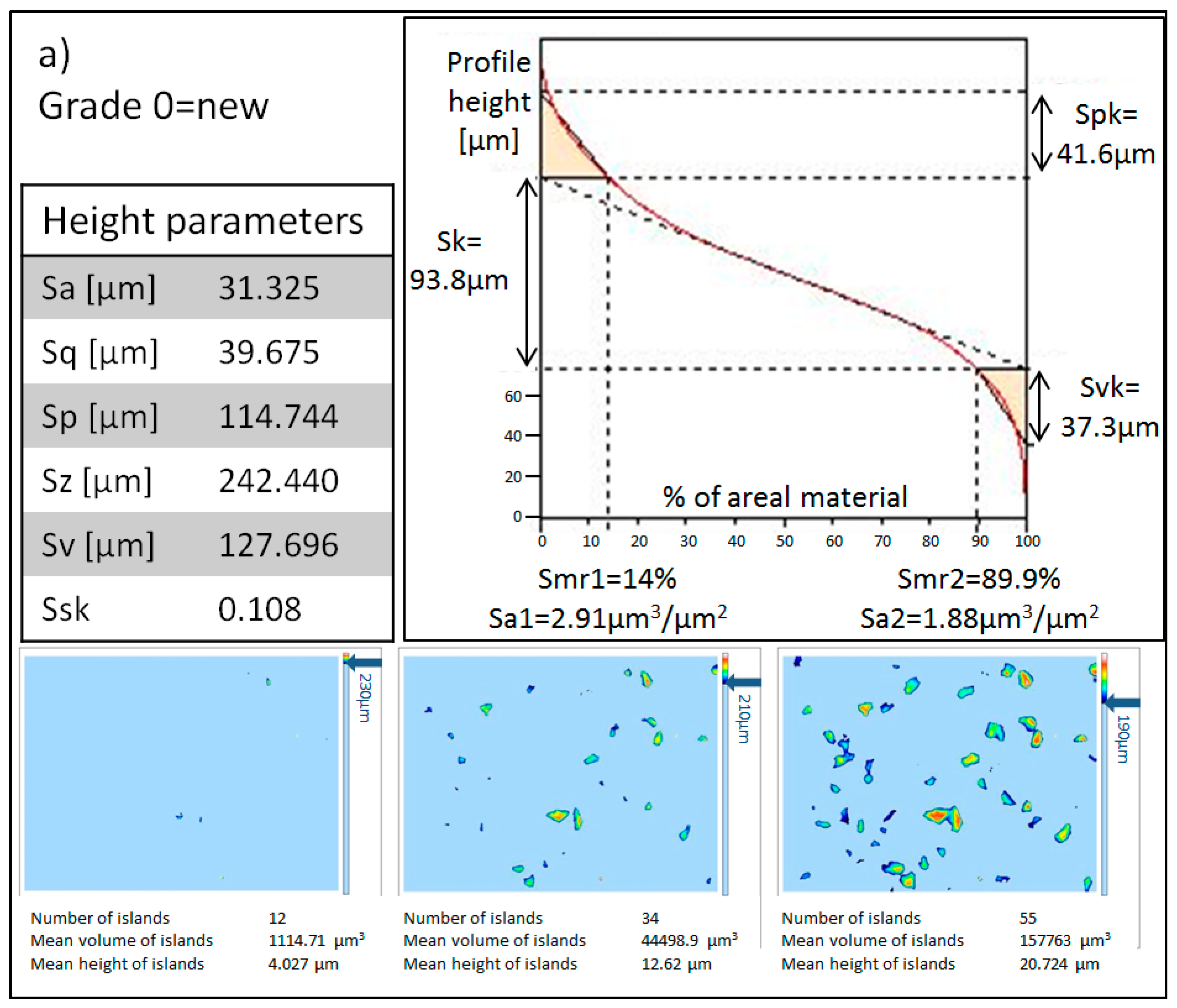
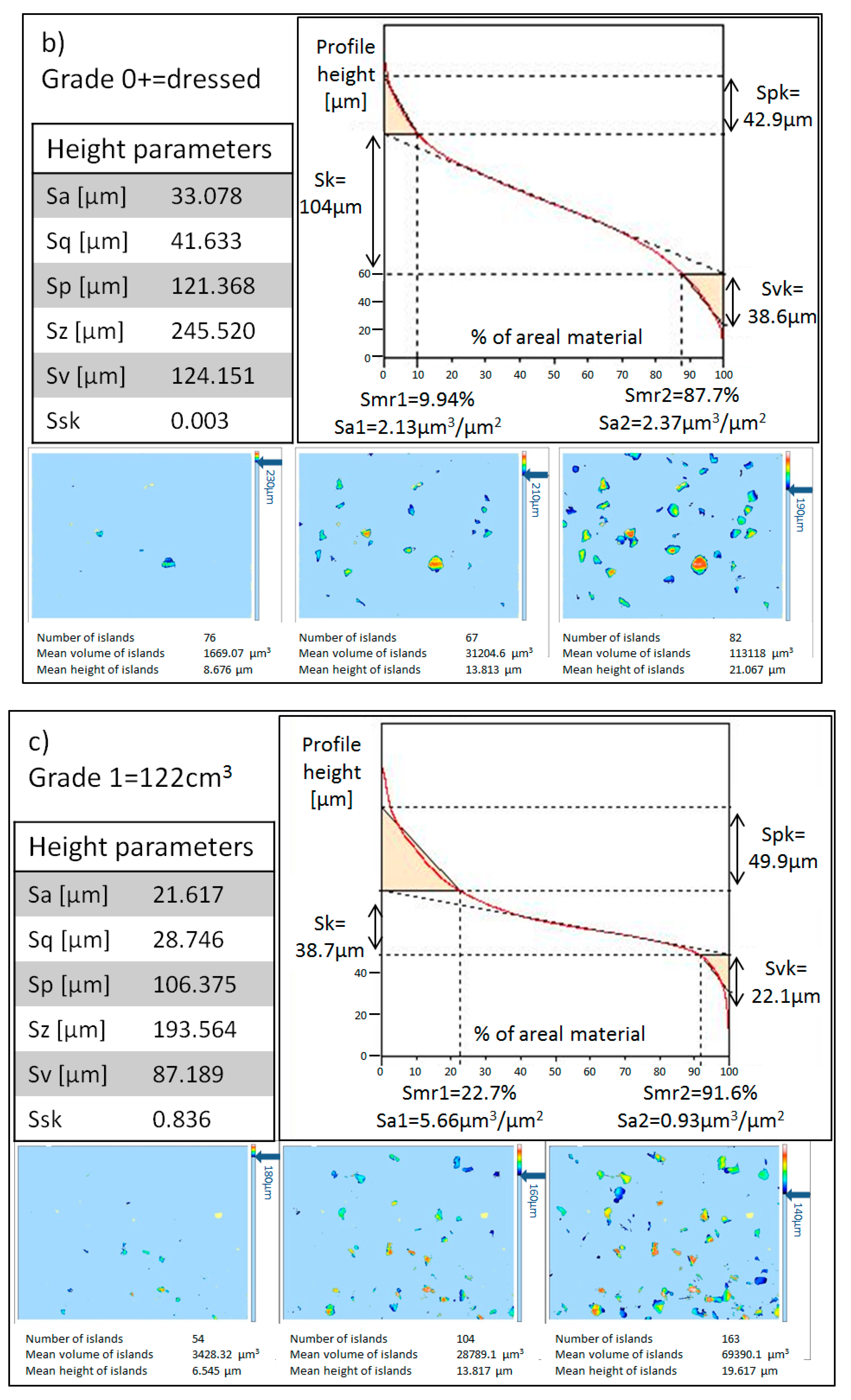
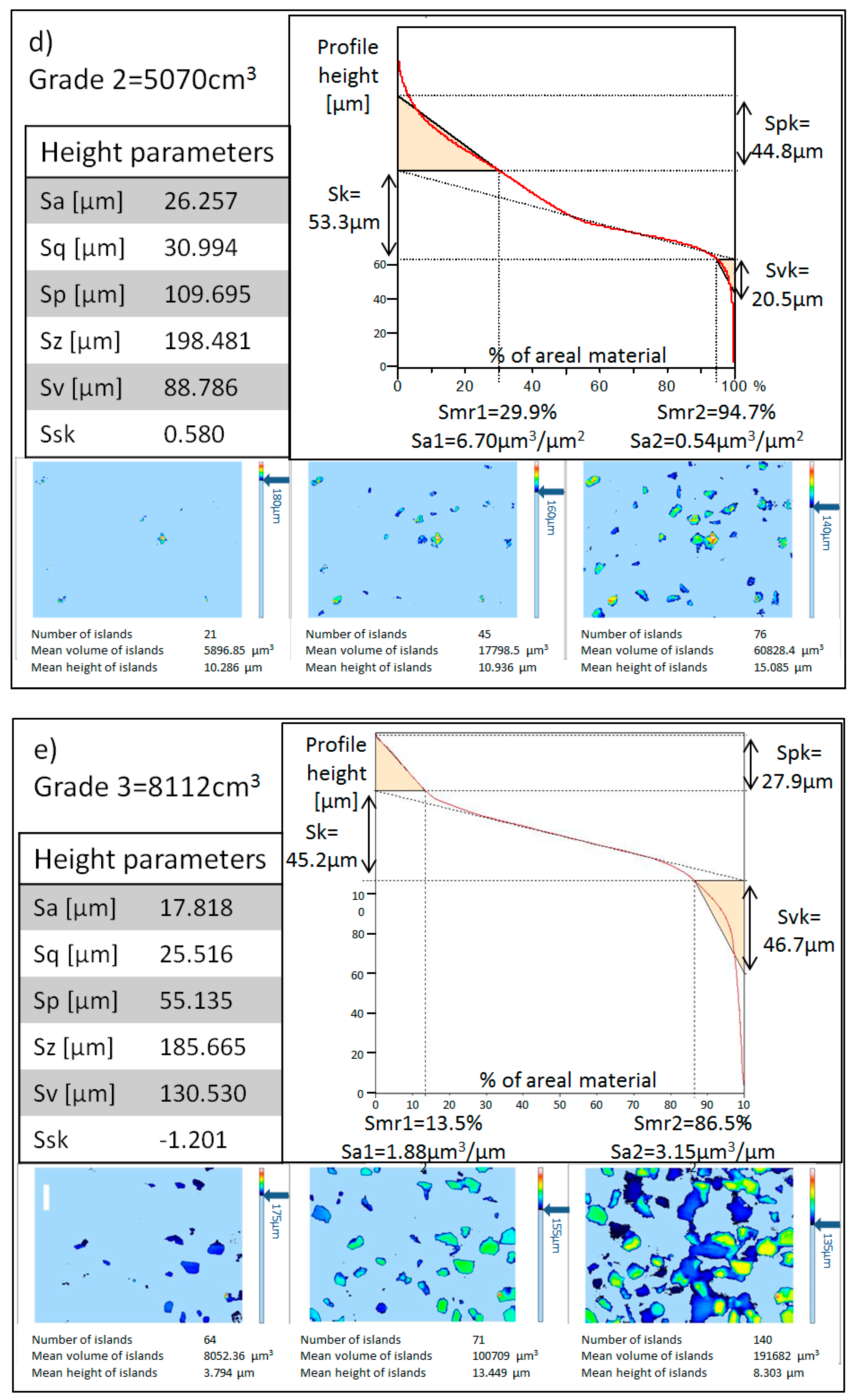
All of these parameters were obtained for the five different wear grades in six different zones along the wheel circumference, that is, every 60°. Figure 8 shows a summary of the study of each grade. In each figure, from Figure 8a to Figure 8e, the following data is depicted, respectively: the parameter table with the height parameters; the Abbott–Firestone curve with the functional parameters; and, below them, three pictures for an optical comparison rather than numerical. The first one (left) shows the upper view of the 3D digitalization of the surface after being digitally sliced with a horizontal plane 10 µm below the highest point; the second one (center) shows the slice at 30 µm; and the last one (right) shows the slice at 50 µm below the highest point.
From the comparison between Figure 8a,b, it can be concluded that the dressing process performed on the new wheel did not have important effects. The greatest noticeable change was the increase in the number of grains due to microfractures that occurred on the grain tips, which can be seen in the slices. In Figure 8c, in the Abbott–Firestone curve, it can be seen that there was a decrease in the profile height, but the upper part was still a similar value to what it was before, which means that the grains were sharp. Figure 8d shows comparable numerical results, but in the last of the slices it can be seen that most of the grains had the same protrusion height, which can be drawn as the beginning of wear flat. Finally, the Abbott–Firestone curve of Figure 8e shows that the upper part of the profile suffered a significant decrease as a consequence of the wear flat. This conclusion can be confirmed with the pictures of the slices.
Nevertheless, the huge number of parameters required a specific methodology for comparing and determining the most representative parameters of the already-detected wear type. A parameter by parameter comparison would lead to tedious work and results that were probably not accurate. As an alternative, the statistical method explained previously was used in this work for a better evaluation of all the parameters.
For a finer adjustment of the threshold value, in this case, the wheel in grade 2 and the wheel in grade 3 were compared. In Table 2 the parameters are sorted according to their significance, from the highest to the lowest values. It should be noted that three different confidence levels were used and that each level led to a different significance value for each parameter and consequently, to a different arrangement.
The skewness resulted in the most significant parameter under every confidence level for detecting the wear flat in the electroplated cBN grinding wheels. The discriminating threshold was established at −0.058, which means that there was a predominance of the valleys. The evolution of Skewness along the wheel life is plotted in Figure 9. It should be mentioned that a symbolic volume of 10 mm3 was given to grade 0+ for separating its dot from grade 0.
From Figure 9, it can be concluded that the wear flat starts being predominant at the end of the wheel life. Nevertheless, different aspects of the whole graphs are discussed in the following lines. The small rise in Skewness in grade 1 and grade 2 means that the peaks are becoming slightly more predominant than the valleys. This can be traced back as a consequence of the progressive microfractures of the grain tips and the progressive transformation of the static grains in dynamic [4]. Some examples of non-touched grains next to fractured grains are gathered in Figure 10. In contrast, the odd change in the Skewness value between grade 2 and grade 3 is because of the significant predominance of the wear flat in grade 3. It should be noted that the accumulated material removal in grade 3 is 1.6 times higher than in grade 2 and that the wear progression does not have to follow a linear expression. If the study had been carried out in intermediate wear states between grade 2 and grade 3, the change would have occurred more progressively.
3.2. Wheel Conditioning Analysis
3.2.1. Topographical Analysis
The use of the same parameter for measuring the change in the wheel topography after the wheel conditioning must be analyzed carefully. The wheel surface is conditioned in order to recover the cutting ability lost due to the grain flattening. However, the grain surface can only be subtly modified since there is only one abrasive layer in the electroplated wheels. Therefore, the average and standard deviation method was applied again to a wheel before and after the conditioning method in order to see the most representative parameter of such a slight change, and thus understand the effect of the conditioning process.
Similarly to the previous analysis, Table 3 arranges the parameters from the highest significance to the lowest.
In comparison with Table 2, the significance values obtained in the conditioning analysis are lower and only positive when the confidence level is 1. This is because the change in the wheel topography is too slight to be detected by the proposed methodology. In consequence, the intervals calculated with the different confidence levels in most of the cases were overlapped, resulting in negative significance values.
Due to the adverse results obtained with the average and standard deviation method, the correlation coefficient was applied as an alternative method. The results of the rGB coefficient are provided in Table 4 and the parameters are arranged from the highest to the lowest value.
Sa is the parameter with the highest coefficient, 0.812, and thus, it is the most representative. However, it gives incomplete information about the surface. For instance, given two equal but inverse surfaces, that is, the valleys of the first surface correspond with the peaks of the second surface and vice versa, the Sa value for them would be the same. As a consequence, a parameter that gives univocal information of the profile would be helpful. Considering that the second parameter with the highest rGB is Sk and that the difference between their coefficients is narrow (0.812 for Sa and 0.800 for Sk), this may be chosen as a complementary and more meaningful roughness parameter. Moreover, Sk gives information about the material distribution along the profile height and it is sensitive to the changes either in the peaks, in the core, or in the valleys. Taking everything into account, Sk was chosen together with Sa as the most representative and meaningful parameters of the change suffered by the grains during the conditioning.
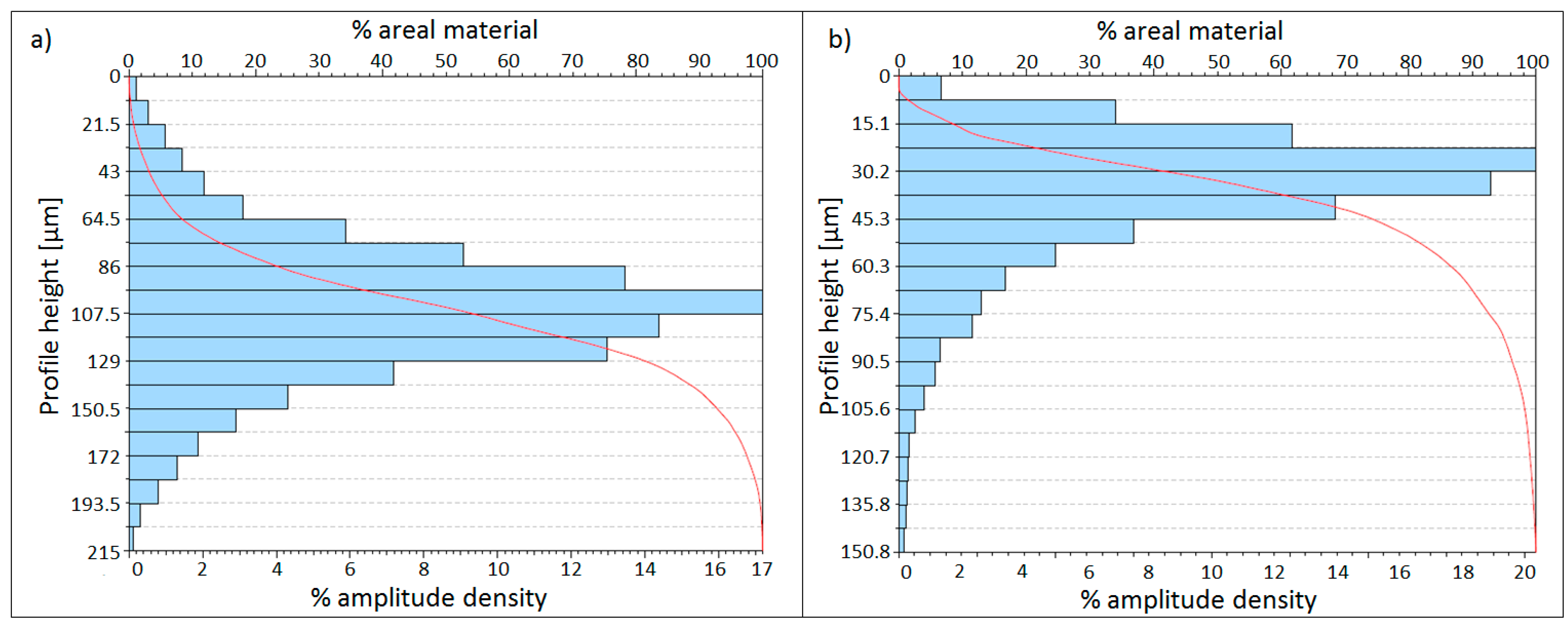
The average value of Sk before conditioning is lower than that after conditioning: 55.2 μm before conditioning versus 58 μm after conditioning. This means that the slope of the equivalent line increases after conditioning. This can be traced back as a consequence of sharpening since there is a lower percentage of material located in the highest part of the profile. An example of this phenomenon can be seen in Figure 11 where the Abbott–Firestone curve of a sharp surface (left) and a blunt surface (right) are compared. In the sharp surface, the probability density function is symmetrical and the slope of the equivalent line would be higher than that of the blunt surface, where the probability density function is displaced upwards. Consequently, a sharp surface would have a higher Sk than a blunt surface. The difference in the scale between the two graphs is caused by the difference in the height of the two profiles. The sharp corresponds to a grade 0 wheel and the blunt to a grade 3 wheel, which has a lower grain protrusion height.
In addition, the increase in the average value of the Sa, 22 μm before conditioning versus 23 μm after conditioning, confirms the presence of a rougher surface after conditioning and also confirms how subtle the change suffered by the wheel was.
3.2.2. Power Consumption
The effect of conditioning in terms of the power consumption was studied by means of four different grinding parameter combinations, from roughing to finishing grinding, as was detailed in Table 1.
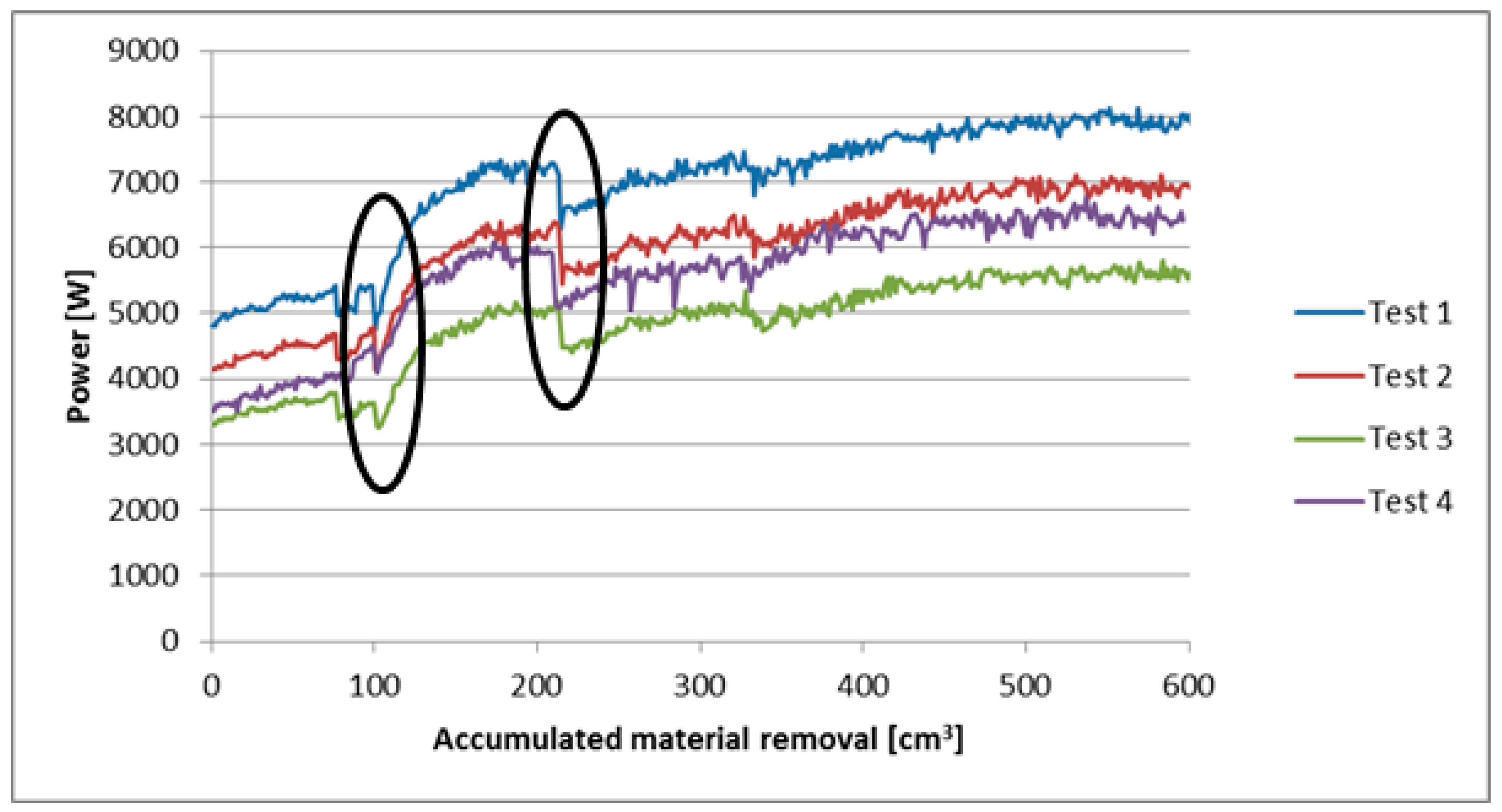
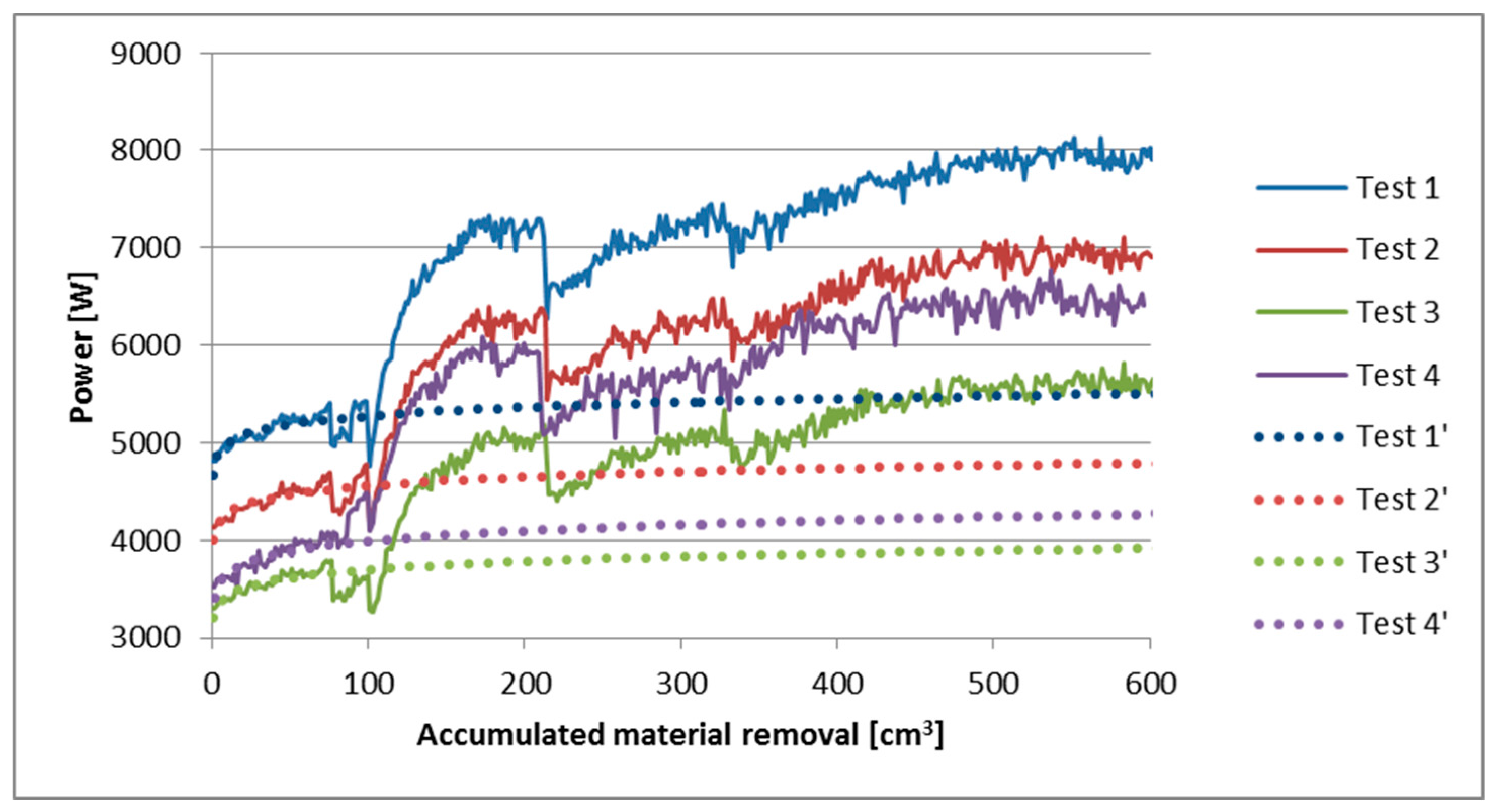
The graph in Figure 12 shows the effect of two conditioning processes marked with black circles. After each one, a sudden decrease in the power consumption was registered as a result of the previously explained sharpening of the grains. However, the signals rapidly suffer an increase, which is higher than the increase that the signals would experience assuming the same progression as before the conditioning. This can be seen in Figure 13 where the curves until the first conditioning are extended by means of the least square method. The extended curves are depicted as dotted lines.
Taking into account the change in the power consumption curve progression, it can be concluded that despite the grain sharpening, the overall wear state of the wheel is accelerated. This is caused by a weakening of the grain tips that soon led to a decrease in the grain height and an increase in the active cutting grains and, eventually, to the appearance of wear flat again.
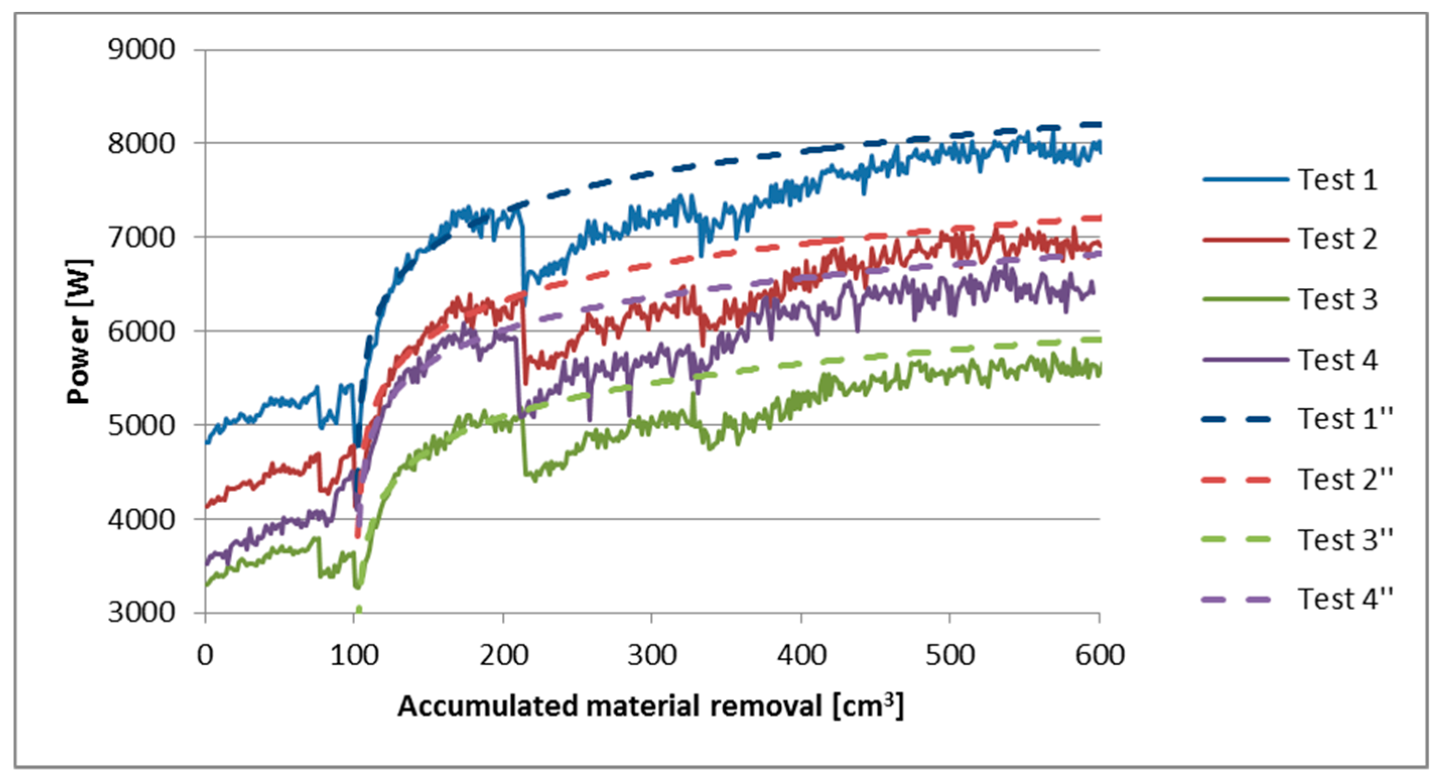
Furthermore, through Figure 14, it can be confirmed that after the first conditioning, the wheel reached a steady wear state where subsequent conditioning processes did not modify the progression of the curve. In Figure 14, the power curve between the first and the second conditioning was extended with slashed lines. These lines finally matched their corresponding power signal after the drop caused by the second sharpening. Hence, conditioning only momentarily modifies the wheel topography before recovering the previous wear state.
Concerning the different parameter combinations proposed for the analysis, a similar sensitivity to the conditioning was seen in different operations. For a full understanding of this phenomenon, it is necessary to have a sense of the actual chip thickness. heq is a widely used parameter for classifying a grinding operation since it takes into account the effect of the cutting speed, feed rate, and cutting depth. However, the result of Equation (12) is not the size of the actual chip thickness, although it is given in µm. The calculation of the actual chip thickness, hcu, has been studied by many authors. Nevertheless, this is not within the scope of this work so the expression for the mean chip thickness of a rectangular chip shape presented by Malkin [28] is used for this explanation. It is shown in Equation (13):
C refers to the active grains density, r refers to the ratio of the chip groove width to chip groove thickness, and de is the equivalent wheel diameter, which, for straight grinding operations, is equal to the wheel diameter. vw, vs, and ae were explained before in this work. Both C and r are parameters difficult to calculate since they depend on the specifications of the wheel, the wheel wear, and the grinding parameters. In this case, an r value equal to 10 [29] and a high active grain density will be used in order to represent the worn state of the wheel. Considering the grain density of the wheel, (see Table 1), and the evenness of the grain height (Figure 8e), an active grain density equal to 12 grains per mm2 was used. The results of the mean chip thickness of the tests from Test1 to Test4 are the following:
- Test1 = 0.58 µm;
- Test2 = 0.53 µm;
- Test3 = 0.53 µm;
- Test4 = 0.58 µm.
From the results, it can be stated that a significant difference in the mean chip thickness of the four tests does not exist. As consequence, all the tests were similarly sensitive to the conditioning process since the interaction between the grains and the workpiece material took place at a similar depth.
It should be mentioned that the work was carried out in an industrial frame. This is why operations with different heq were planned instead of operations with different hcu.
4. Conclusions
The surface of the electroplated cBN grinding wheels during the CFG of aeronautic components made of C1023 was analyzed at different wear states. Wear flat was found as the main wear type in the advanced wear states of the wheel. This was the cause of the problems detected in some specific parts of the NGV as well.
The average and standard deviation method was applied to the roughness parameters from the digitalization of the grinding wheel topography under different wear states. Thanks to that method, the most representative parameter for recognizing the presence of wear flat and the threshold for classifying a worn wheel were obtained. The Ssk resulted in the most significant parameter and, according to the empirical experience, the threshold was set as −0.058.
The conditioning process used as a solution for the problems caused by the wear in some specific zones of the NGV was assessed in terms of wheel topography and power consumption.
For that purpose, the wheel was digitalized before and after conditioning and the average and standard deviation method was applied to the results. However, the modification was too slight to be detected by this method and the correlation coefficient method was used as an alternative. Sa and Sk resulted in the most significant parameters of the change caused by the conditioning. On the one side, the increase in the average value of Ra confirmed a rougher surface after conditioning. On the other, the increase in Sk average value was traced back as a result of the grain sharpening and the consequent increase in the slope of the equivalent line.
The sharpening of the grains was confirmed with the power consumption analysis since, after each conditioning, the power consumption decreased. Nevertheless, it was also observed that the wear state of the wheel was accelerated by the conditioning. The progression outlined by the curve before the conditioning was extended to be compared with the actual power consumption. The result was that the actual power consumption clearly exceeded the extended curve.
However, after the first conditioning, in spite of being conditioned again, the power signal returned to the same progression. This is because the transitory state where the passive grains were becoming active grains was overtaken by the conditioning. As a result, from that point on, the conditioning only modified the tip of the grains momentarily before the wheel returned to a similar wear state.
Finally, the wheel behavior in terms of the power consumption was the same for the four different heq values. This means that the contact between the grain and the workpiece occurred at a very shallow depth and that the influence of conditioning was equally noticeable for the roughing and finishing operations, as can be confirmed by the results of Equation (13).
Author Contributions
H.B. conducted the experiments. G.V. carried out the wheel topography analysis. H.G. statistically analyzed the roughness parameters. N.O. wrote the manuscript. M.D. supervised the work and revised the article.
Acknowledgements
The authors gratefully acknowledge the funding support received from the Spanish Ministry of Economy and Competitiveness and the FEDER operation program for funding the project “Optimización de procesos de acabado para componentes críticos de aerorreactores” (DPI2014-56137-C2-1-R).
Conflicts of Interest
The authors declare no conflict of interest. The founding sponsors had no role in the design of the study; in the collection, analyses, or interpretation of data; in the writing of the manuscript, and in the decision to publish the results.
References
- Boyer, R. Aircraft Materials. In Encyclopedia of Materials: Science and Technology, 2nd ed.; Elsevier: New York, NJ, USA, 2001; pp. 66–73. ISBN 978-008-043152-9. [Google Scholar]
- Giampaolo, T. The Gas Turbine Handbook: Principles and Practice, 3rd ed.; The Fairmont Press: Lilburn, GA, USA, 2003; ISBN 0881735159. [Google Scholar]
- Marinescu, I.; Hitchiner, M.; Uhlmann, E. Handbook of Machining with Grinding Wheels; Taylor & Francis Group: Boca Raton, FL, USA, 2006; ISBN 9781574446715. [Google Scholar]
- Marinescu, I.D.; Rowe, W.B.; Dimitrov, B.; Inasaki, I. Tribology of Abrasive Machining Processe; William Andrew: Norwich, NY, USA, 2004; ISBN 0-8155-1490-5. [Google Scholar]
- Ding, W.; Barbara, L.; Zhu, Y.; Li, Z.; Fu, Y.; Su, H.; Xu, J. Review on monolayer cBN superabrasive wheels for grinding metallic materials. Chin. J. Aeronaut. 2017, 30, 109–134. [Google Scholar] [CrossRef]
- Wegener, K.; Hoffmeister, H.W.; Karpuschewski, B.; Kuster, F.; Hahmann, W.C.; Rabiey, M. Conditioning and monitoring of grinding wheels. CIRP Ann. Manuf. Technol. 2011, 60, 757–777. [Google Scholar] [CrossRef]
- Brinksmeier, E.; Werner, F. Monitoring of Grinding Wheel Wear. CIRP Ann. Manuf. Technol. 1992, 41, 373–376. [Google Scholar] [CrossRef]
- Furutani, K.; Ohguro, N.; Hieu, N.T.; Nakamura, T. In-process measurement of topography change of grinding wheel by using hydrodynamic pressure. Int. J. Mach. Tools Manuf. 2002, 42, 1447–1453. [Google Scholar] [CrossRef]
- Furutani, K.; Trong Hieu, N.; Ohguro, N.; Nakamura, T. Automatic compensation for grinding wheel wear by pressure based in-process measurement in wet grinding. Precis. Eng. 2003, 27, 9–13. [Google Scholar] [CrossRef]
- Sutowski, P.; Plichta, S. An investigation of the grinding wheel wear with the use of root-mean-square value of acoustic emission. Arch. Civ. Mech. Eng. 2006, 6, 87–98. [Google Scholar] [CrossRef]
- Liao, T.W.; Tang, F.; Qu, J.; Blau, P.J. Grinding wheel condition monitoring with boosted minimum distance classifiers. Mech. Syst. Signal Process. 2008, 22, 217–232. [Google Scholar] [CrossRef]
- Blunt, L.; Ebdon, S. The application of three-dimensional surface measurement techniques to characterizing grinding wheel topography. Int. J. Mach. Tools Manuf. 1996, 36, 1207–1226. [Google Scholar] [CrossRef]
- Butler, D.; Blunt, L.; See, B.; Webster, J.; Stout, K. The characterisation of grinding wheels using 3D surface measurement techniques. J. Mater. Process. Technol. 2002, 127, 234–237. [Google Scholar] [CrossRef]
- Shi, Z.; Malkin, S. Wear of Electroplated cBN Grinding Wheels. J. Manuf. Sci. Eng. 2006, 128, 110. [Google Scholar] [CrossRef]
- Upadhyaya, R.P.; Fiecoat, J.H. Factors Affecting Grinding Performance with Electroplated cBN Wheels. CIRP Ann. Manuf. Technol. 2007, 56, 339–342. [Google Scholar] [CrossRef]
- Guo, C.; Shi, Z.; Attia, H.; McIntosh, D. Power and Wheel Wear for Grinding Nickel Alloy with Plated cBN Wheels. CIRP Ann. Manuf. Technol. 2007, 56, 343–346. [Google Scholar] [CrossRef]
- Ding, W.F.; Xu, J.H.; Chen, Z.Z.; Su, H.H.; Fu, Y.C. Wear behavior and mechanism of single-layer brazed cBN abrasive wheels during creep-feed grinding cast nickel-based superalloy. Int. J. Adv. Manuf. Technol. 2010, 51, 541–550. [Google Scholar] [CrossRef]
- Yu, T.; Bastawros, A.F.; Chandra, A. Experimental Characterization of Electroplated Cbn Grinding Wheel Wear: Topology Evolution and Interfacil Toughness. In Proceedings of the ASME 2014 International Manufacturing Science and Engineering Conference, Detroit, MI, USA, 9–13 June 2014; pp. 1–8. [Google Scholar]
- Ye, R.; Jiang, X.; Blunt, L.; Cui, C.; Yu, Q. The application of 3D-motif analysis to characterize diamond grinding wheel topography. Meas. J. Int. Meas. Confed. 2016, 77, 73–79. [Google Scholar] [CrossRef]
- Ghosh, A.; Chattopadhyay, A.K. Experimental investigation on performance of touch-dressed single-layer brazed cBN wheels. Int. J. Mach. Tools Manuf. 2007, 47, 1206–1213. [Google Scholar] [CrossRef]
- Ghosh, A.; Chattopadhyay, A.K. On cumulative depth of touch-dressing of single layer brazed cbn wheels with regular grit distribution pattern. Mach. Sci. Technol. 2007, 11, 259–270. [Google Scholar] [CrossRef]
- Zhao, Q.; Guo, B. Ultra-precision grinding of optical glasses using mono-layer nickel electroplated coarse-grained diamond wheels. Part 1: ELID assisted precision conditioning of grinding wheels. Precis. Eng. 2015, 39, 56–66. [Google Scholar] [CrossRef]
- Kitzig, H.; Tawakoli, T.; Azarhoushang, B. A novel ultrasonic-assisted dressing method of electroplated grinding wheels via stationary diamond dresser. Int. J. Adv. Manuf. Technol. 2016, 86, 487–494. [Google Scholar] [CrossRef]
- Dold, C.; Transchel, R.; Rabiey, M.; Langenstein, P.; Jaeger, C.; Pude, F.; Kuster, F.; Wegener, K. A study on laser touch dressing of electroplated diamond wheels using pulsed picosecond laser sources. CIRP Ann. Manuf. Technol. 2011, 60, 363–366. [Google Scholar] [CrossRef]
- Pfaff, J.; Warhanek, M.; Huber, S.; Komischke, T.; Hänni, F.; Wegener, K. Laser Touch Dressing of Electroplated cBN Grinding Tools. Procedia CIRP 2016, 46, 272–275. [Google Scholar] [CrossRef]
- Leach, R. Characterization of Areal Surface Texture; Springer: London, UK, 2013; ISBN 978-3-642-36458-7. [Google Scholar]
- Arantes, L.J.; Fernandes, K.A.; Schramm, C.R.; Silveire Leal, J.E.; Piratelli-Filho, A.; Domingues Franco, S.; Valdes Arancibia, R. The roughness characterization in cylinders obtained by conventional and flexible honing processes. Int. J. Adv. Manuf. Technol. 2017, 93, 635–649. [Google Scholar] [CrossRef]
- Malkin, S.; Guo, C. Grinding Technology: Theory and Application of Machining with Abrasives; Industrial Press Inc.: New York, NY, USA, 2008; ISBN 978-0-8311-3247-7. [Google Scholar]
- Mayer, J.E.; Fang, G.P.; Kegg, R.L. Effect of Grit Depth of Cut on Strength of Ground Ceramics. CIRP Ann. Manuf. Technol. 1994, 43, 309–312. [Google Scholar] [CrossRef]
Figure 1.
The distribution in weight of the structural materials used for the Boeing 747, 777, and C-17 [1].
Figure 1.
The distribution in weight of the structural materials used for the Boeing 747, 777, and C-17 [1].

Figure 2.
The nozzle guide vane (NGV) and its composition.

Figure 3.
The geometry of the inner rail on a nozzle guide vane and of the grinding wheel. (a) The inner rail, marked in red in the NGV; (b) A depiction of the grinding operation of the inner rail. The abrasive surface of the grinding wheel is marked in brown, while the green arrow indicates the path of the wheel along the inner rail.

Figure 4.
The vibration marks appear marked with the slashed rectangles and the thermally damaged zones are marked with the orange ovals.
Figure 4.
The vibration marks appear marked with the slashed rectangles and the thermally damaged zones are marked with the orange ovals.

Figure 5.
(a) A grinding wheel together with the HSK clamping system, digitalized in the confocal microscope. (b) The surface of the grinding wheel displayed through the Leicamap®. (c) The roughness parameters according to the ISO 25178 standard. (d) The Abbott–Firestone curve or material bearing the area curve where functional parameters can be obtained. (e) A slice of the digitalized surface where the analysis can be focused on the grain tips.

Figure 6.
(a,c): the surface of a wheel in grade 0. (b,d): the surface of a wheel in grade 3. In orange there are some wear flats. (e,g): two mirror-like flat grains observed by an optical macroscope and a scanning electron microscope (SEM), respectively. (f,h): two rough flat grains, named wear flats, observed by an optical macroscope and an SEM.

Figure 7.
The Abbott–Firestone curve.

Figure 8.
An example of the studies carried out during each grade of the wheel. The subfigures from (a–e) correspond to grades 0 to 3, respectively. In each figure from (a–e) there are the following: the name of the grade and the corresponding accumulated material removal; a table with the values of the height parameters; the Abbott–Firestone diagram together with the functional parameters; and finally, three pictures of the surface sliced digitally at three different heights, namely 10 µm (left), 30 µm (center), and 50 µm (right) below the highest point of the surface.


Figure 9.
The Ssk value corresponding with the five wear states of the wheel.

Figure 10.
The SEM pictures of fractured grains next to untouched grains.

Figure 11.
(a) The Abbott–Firestone curve of a sharp surface; (b) the Abbott–Firestone curve of a blunt surface.
Figure 11.
(a) The Abbott–Firestone curve of a sharp surface; (b) the Abbott–Firestone curve of a blunt surface.

Figure 12.
The power consumption of the four tests during the first 600 cm3 of removed material. The black circles mark the two conditioning processes.
Figure 12.
The power consumption of the four tests during the first 600 cm3 of removed material. The black circles mark the two conditioning processes.

Figure 13.
The power consumption of the four tests during the first 600 cm3 of removed material. The lines in dots are the extensions of the curve before the first conditioning.
Figure 13.
The power consumption of the four tests during the first 600 cm3 of removed material. The lines in dots are the extensions of the curve before the first conditioning.

Figure 14.
The power consumption of the four tests during the first 600 cm3 of removed material. The slashed lines are the extensions of the curve before the first conditioning.
Figure 14.
The power consumption of the four tests during the first 600 cm3 of removed material. The slashed lines are the extensions of the curve before the first conditioning.


Table 1.
The details of the study for the conditioning process. cBN: cubic boron nitride; heq: equivalent chip thickness; SiC: silicon carbide.
Table 1.
The details of the study for the conditioning process. cBN: cubic boron nitride; heq: equivalent chip thickness; SiC: silicon carbide.
| Wheel diameter | 150 mm | |||
| cBN grain size | 250 µm | |||
| Grain density | ≈14 grains/cm2 | |||
| Workpiece material | C1023 (nickel base superalloy) | |||
| Grinding speed | 80 m/s | |||
| Test name | Test1 | Test2 | Test3 | Test4 |
| Depth of cut (mm) | 0.4 | 0.3 | 0.15 | 0.15 |
| Feed rate (mm/min) | 630 | 605 | 850 | 1040 |
| heq (µm) | 3.15 | 2.27 | 1.6 | 1.95 |
| Cutting fluid | Oil-based high pressure | |||
| SiC grain size | 68 μm | |||
Table 2.
The significance of each parameter under different levels of confidence for the study of wheel wear.
Table 2.
The significance of each parameter under different levels of confidence for the study of wheel wear.
| k = 1 | k = 2 | k = 3 | |||
|---|---|---|---|---|---|
| Parameters | Significance | Parameters | Significance | Parameters | Significance |
| Ssk (-) | 6.396 | Ssk | 4.776 | Ssk | 3.157 |
| Sa1 (µm3/mm2) | 1.143 | Sa1 | 0.642 | Smr1 | 0.384 |
| Sa2 (µm3/mm2) | 1.010 | Smr1 | 0.610 | Svk | 0.262 |
| Smr1 (%) | 0.837 | Sa2 | 0.514 | Sp | 0.230 |
| Spk (µm) | 0.630 | Svk | 0.444 | Sa1 | 0.140 |
| Svk (µm) | 0.625 | Sp | 0.400 | Sa2 | 0.018 |
| Sp (µm) | 0.570 | Spk | 0.127 | Smr2 | −0.021 |
| Sa (µm) | 0.111 | Smr2 | 0.033 | Sa | −0.179 |
| Smr2 (%) | 0.087 | Sq | −0.130 | Sz | −0.329 |
| Sz (µm) | 0.058 | Sz | −0.136 | Spk | −0.375 |
| Sq (µm) | 0.013 | Sv | −0.323 | Sv | −0.559 |
| Sv (µm) | −0.088 | Sku | −0.329 | Sk | −0.753 |
| Sk (µm) | −0.232 | Sk | −0.492 | Sku | −0.761 |
Table 3.
The significance of each parameter under different levels of confidence for the study of wheel conditioning.
Table 3.
The significance of each parameter under different levels of confidence for the study of wheel conditioning.
| k = 1 | k = 2 | k = 3 | |||
|---|---|---|---|---|---|
| Parameters | Significance | Parameters | Significance | Parameters | Significance |
| Sv | 0.074 | Sz | −0.064 | Smr2 | −0.102 |
| Sz | 0.060 | Smr2 | −0.066 | Sz | −0.188 |
| Sp | −0.020 | Sku | −0.112 | Sv | −0.238 |
| Smr2 | −0.031 | Sp | −0.166 | Sp | −0.311 |
| Spk | −0.079 | Spk | −0.277 | Spk | −0.474 |
| Sq | −0.154 | Sq | −0.334 | Sq | −0.515 |
| Sa | −0.158 | Sa | −0.359 | Sa | −0.560 |
| Svk | −0.194 | Smr1 | −0.482 | Smr1 | −0.754 |
| Smr1 | −0.210 | Sk | −0.488 | Sk | −0.757 |
| Sk | −0.219 | Svk | −0.520 | Svk | −0.845 |
| Sa2 | −0.304 | Sa2 | −0.784 | Sa2 | −1.263 |
| Sa1 | −0.626 | Sa1 | −1.412 | Sa1 | −2.198 |
| Ssk | −1.351 | Ssk | −4.000 | Ssk | −6.650 |
Table 4.
The correlation coefficient of each parameter for the study of wheel conditioning.
| Parameters | rGB |
|---|---|
| Sa | 0.812 |
| Sk | 0.800 |
| Sz | 0.744 |
| Smr1 | 0.739 |
| Svk | 0.685 |
| Smr2 | 0.632 |
| Sq | 0.625 |
| Sv | 0.448 |
| Sp | 0.164 |
| Sa1 | 0.126 |
| Ssk | −0.095 |
| Spk | −0.129 |
| Sa2 | −0.211 |
© 2018 by the authors. Licensee MDPI, Basel, Switzerland. This article is an open access article distributed under the terms and conditions of the Creative Commons Attribution (CC BY) license (http://creativecommons.org/licenses/by/4.0/).
Share and Cite
MDPI and ACS Style
Vidal, G.; Ortega, N.; Bravo, H.; Dubar, M.; González, H. An Analysis of Electroplated cBN Grinding Wheel Wear and Conditioning during Creep Feed Grinding of Aeronautical Alloys. Metals 2018, 8, 350. https://doi.org/10.3390/met8050350
AMA Style
Vidal G, Ortega N, Bravo H, Dubar M, González H. An Analysis of Electroplated cBN Grinding Wheel Wear and Conditioning during Creep Feed Grinding of Aeronautical Alloys. Metals. 2018; 8(5):350. https://doi.org/10.3390/met8050350
Chicago/Turabian StyleVidal, Gorka, Naiara Ortega, Héctor Bravo, Mirentxu Dubar, and Haizea González. 2018. "An Analysis of Electroplated cBN Grinding Wheel Wear and Conditioning during Creep Feed Grinding of Aeronautical Alloys" Metals 8, no. 5: 350. https://doi.org/10.3390/met8050350
Note that from the first issue of 2016, this journal uses article numbers instead of page numbers. See further details here.