Strain Rate Contribution due to Dynamic Recovery of Ultrafine-Grained Cu–Zr as Evidenced by Load Reductions during Quasi-Stationary Deformation at 0.5 Tm


Abstract
1. Introduction
- demonstrate that the transient response to load changes can be studied in standard tensile creep machines with load control,
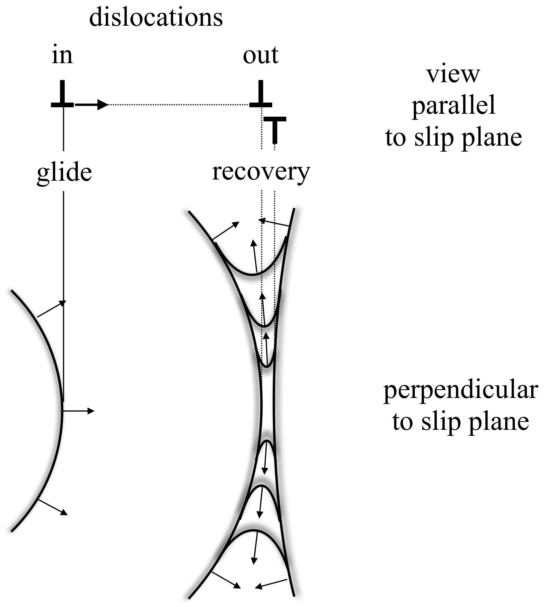
- show that the transient behavior of an ufg material is qualitatively the same as that of cg materials, including an initial period of strain mainly due to recovery,
- discuss the mechanism of dynamic recovery in qs and transient deformation with special regard to the influence of internal stresses.
2. Experimental Details
3. Results
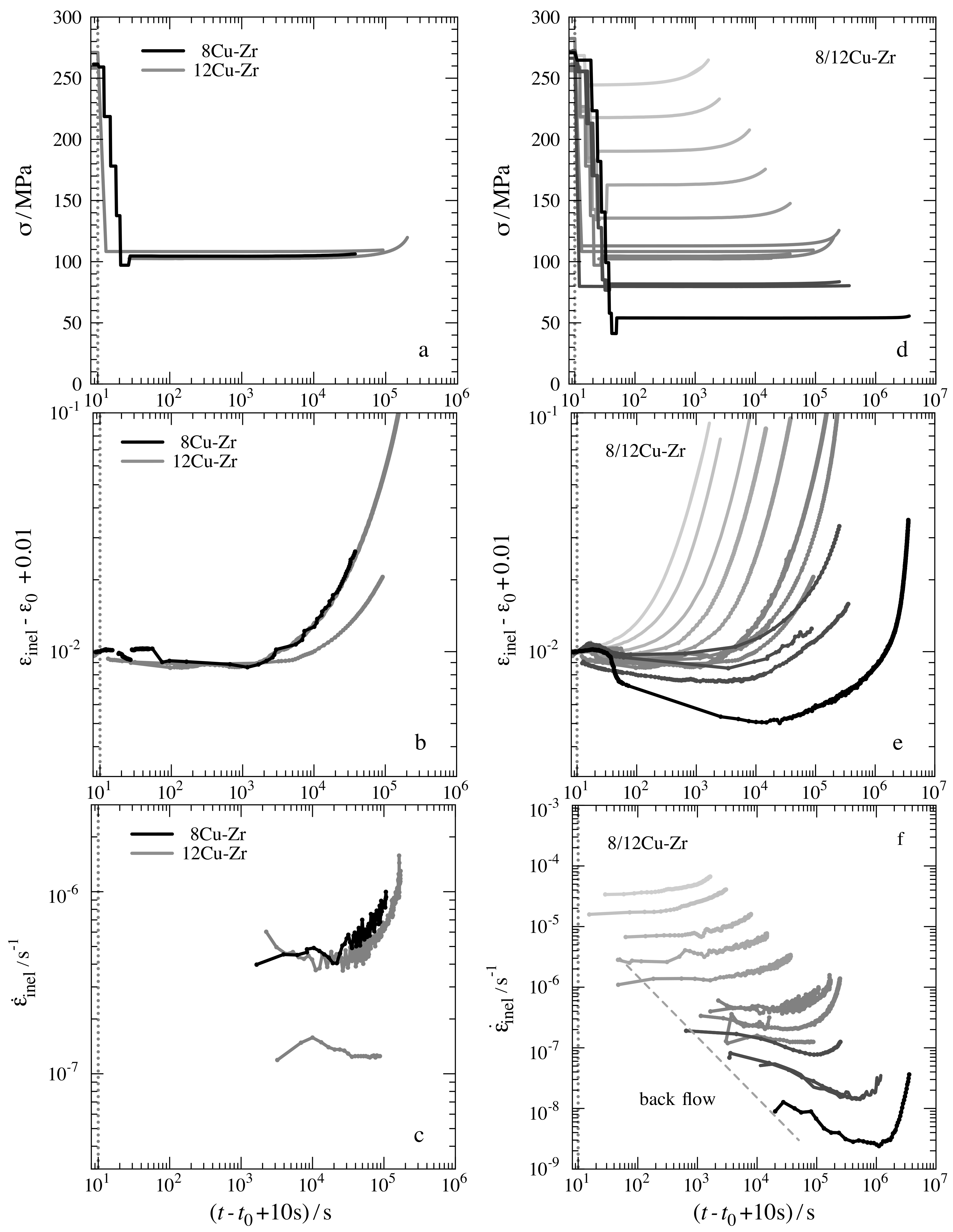
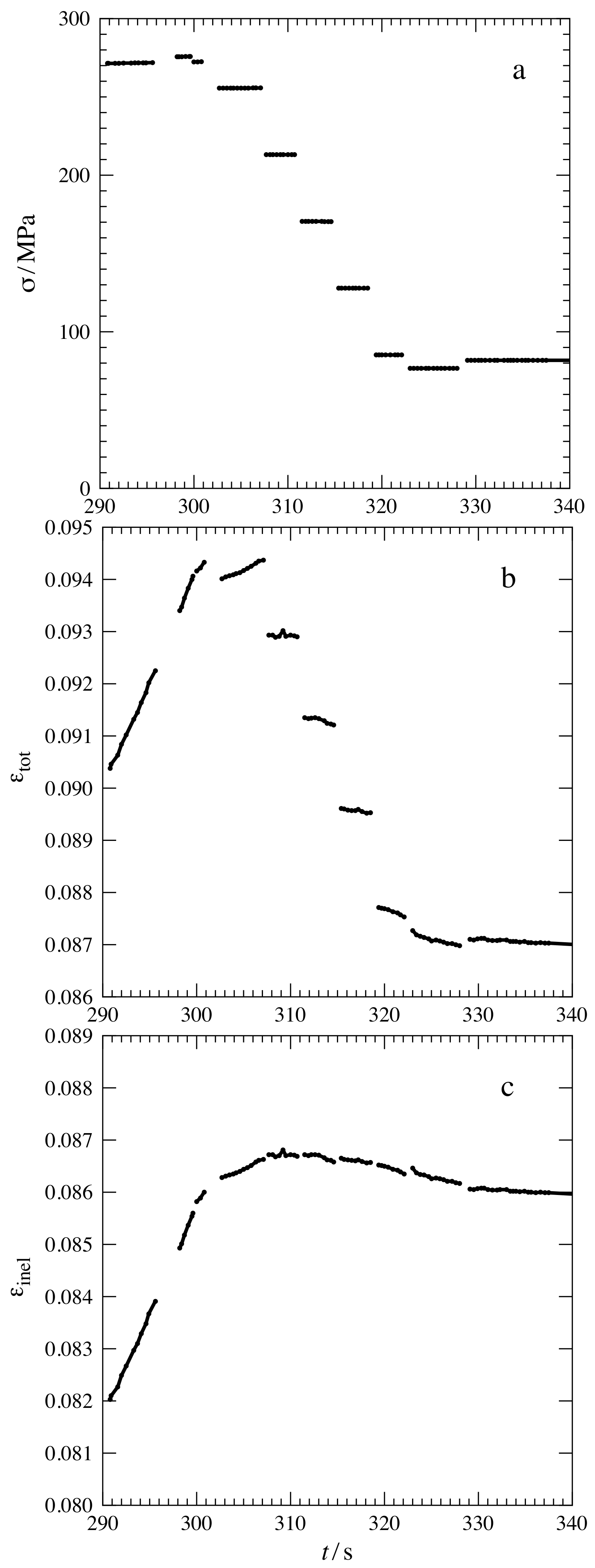
3.1. Transients as Function of Time
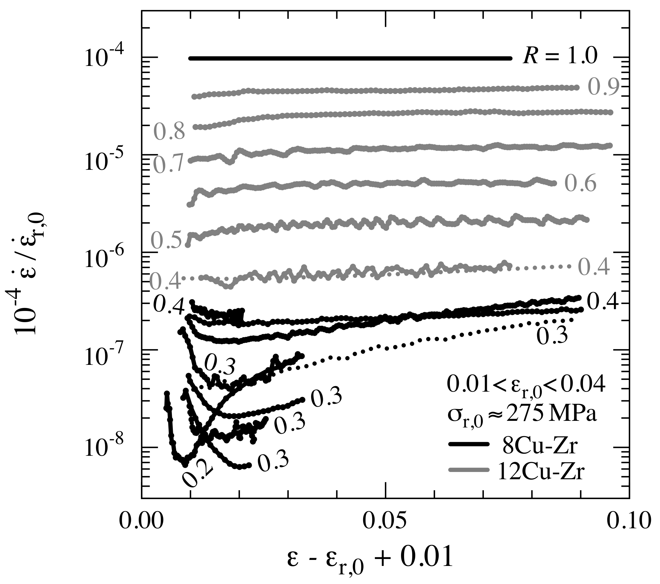
3.2. Transients as Function of Strain
4. Discussion
4.1. Strain Related with Storage of Defects
4.2. Strain Related with Recovery of Defects
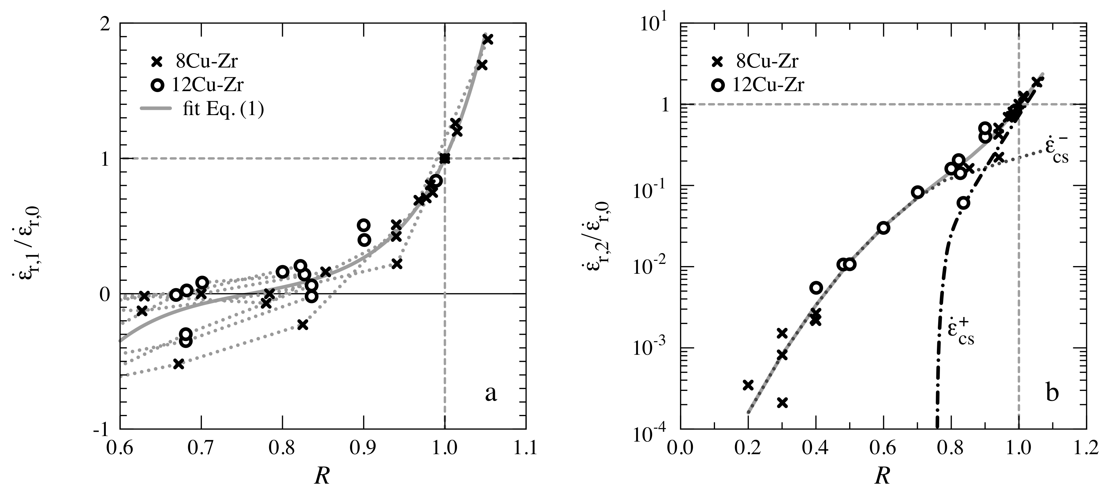
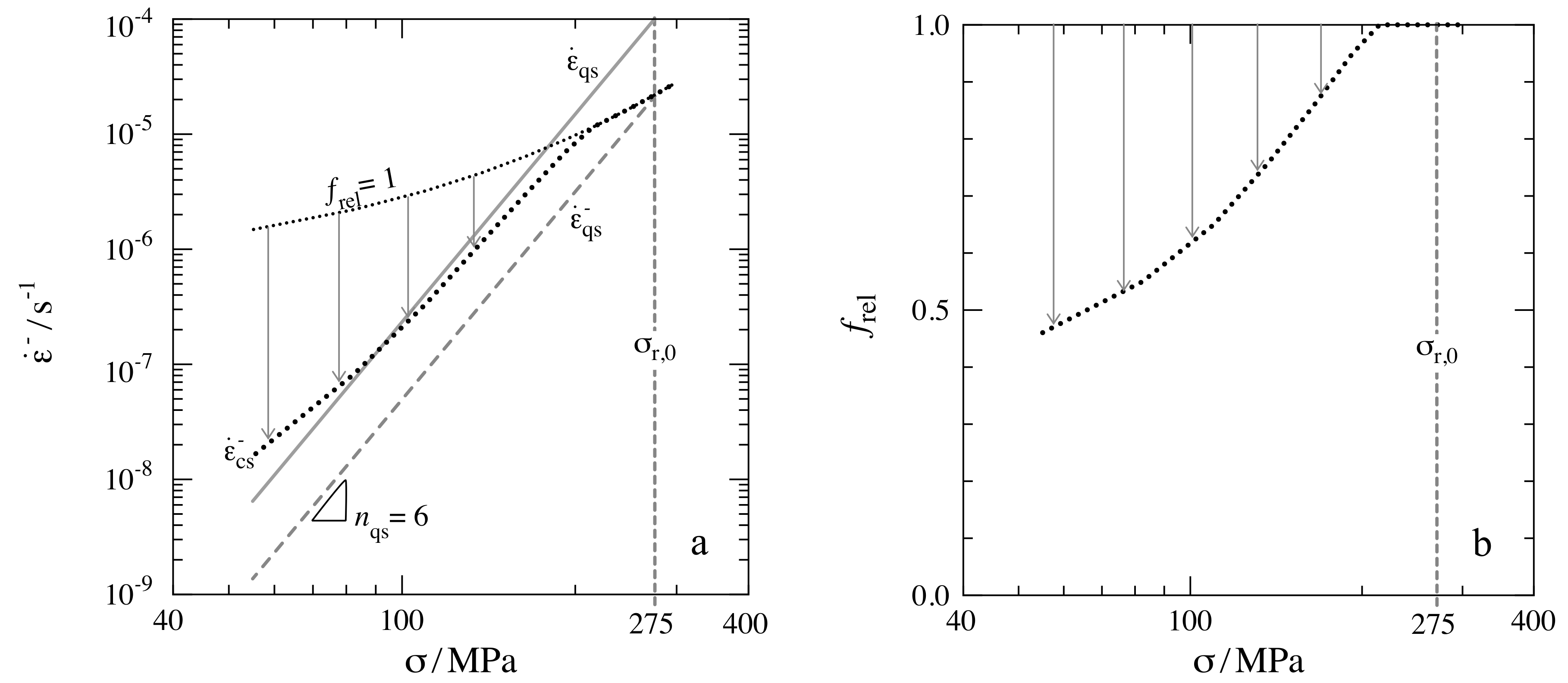
4.3. Comparison of Stress Dependences of and at Constant Structure
5. Summary
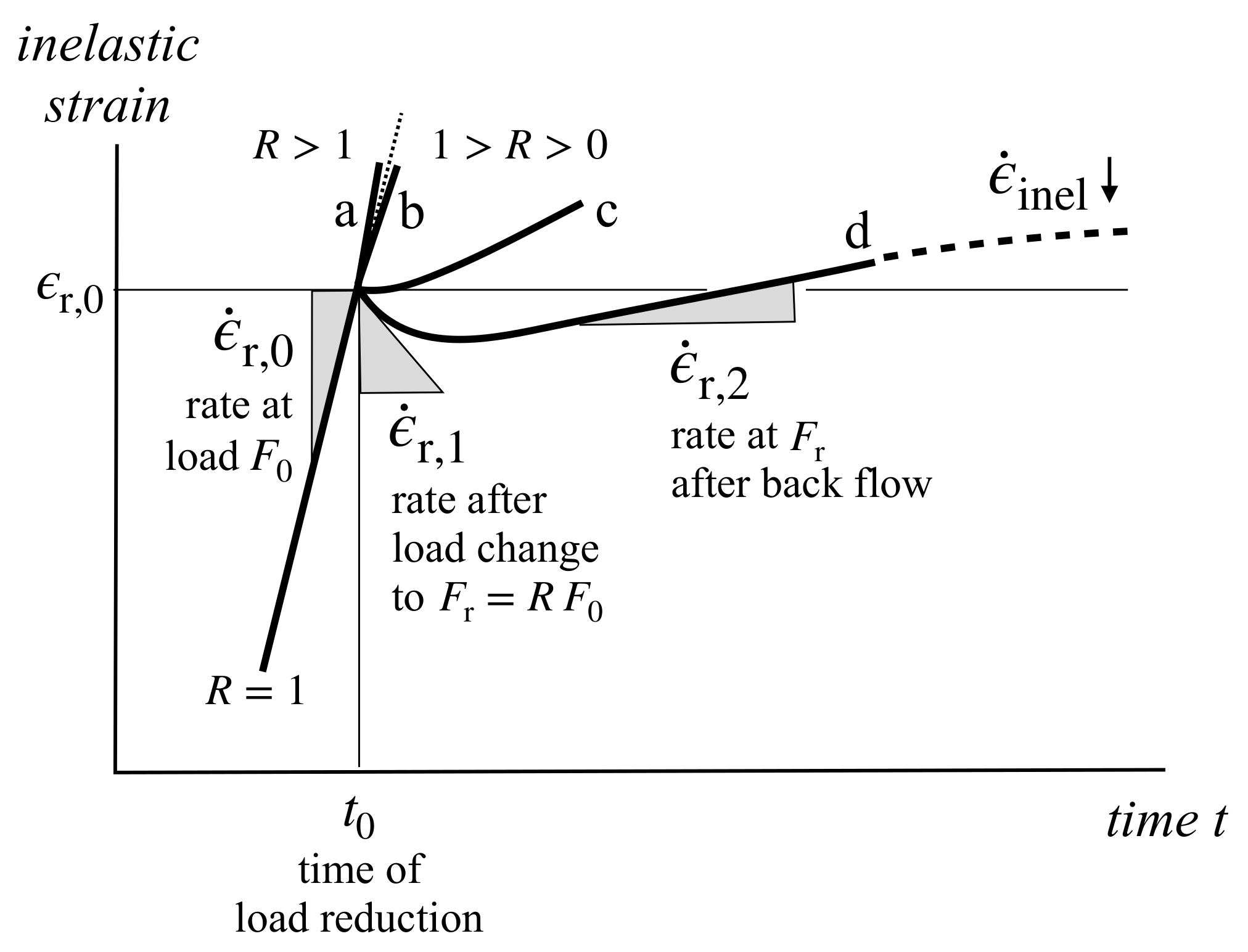
- In ufg Cu–Zr at recovery–strain connected with dynamic recovery of strain-induced crystal defects was found in tests with perturbation of the quasi-stationary (qs) state by load reductions. adds to the strain connected with dislocation generation and storage.
- The stress dependence of yields an activation volume consistent with the classical theory of thermally activated glide.
- The recovery–strain rate contributes 10% to 30% to the quasi-stationary strain rate . This fraction for ufg Cu–Zr with high volume fraction of HABs is similar to the one commonly reported for cg materials with high volume fraction of LABs. That could mean that boundaries play qualitatively similar roles in mediating dynamic recovery independent of their misorientation.
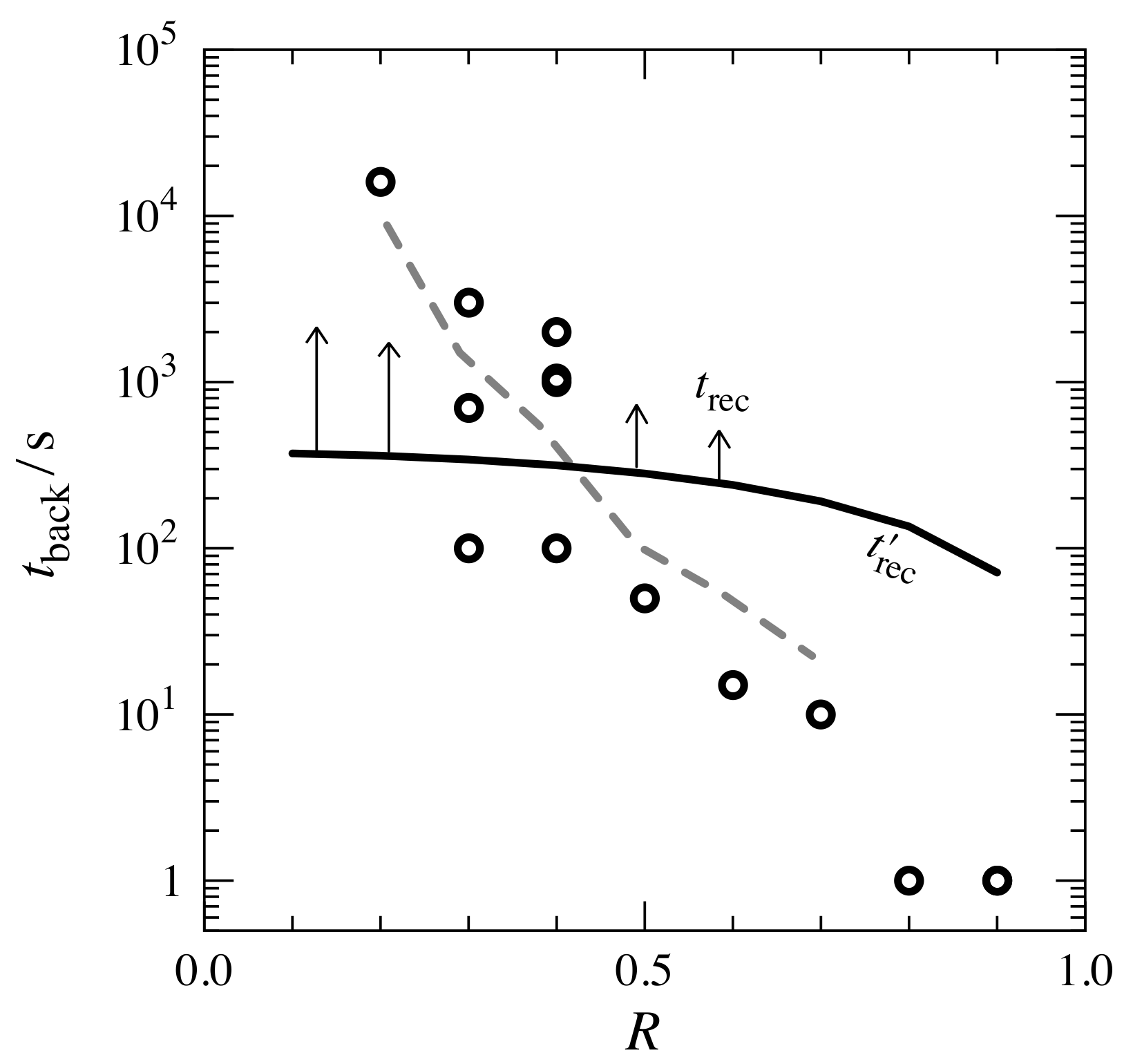
- The values of (at constant structure) and (at quasi-stationary structure) are relatively similar for large load reductions, even though the microstructures, in particular the dislocation structures, should differ significantly. This becomes understandable, if promotion of recovery by internal forward stresses is taken into account.
- Combining the rates of recovery–strain in the qs state and after perturbation of monotonic flow seems promising to better understand the mechanism of dynamic recovery of crystal defects, limiting the deformation strength under monotonic as well as cyclic loading conditions.
Author Contributions
Conflicts of Interest
Abbreviations
| qs | quasi-stationary |
| ECAP | equal channel angular pressing |
| cg | coarse-grained |
| ufg | ultrafine-grained |
| LAB | low-angle boundary |
| HAB | high-angle boundary |
Appendix A. Determination of Inelastic Strain

Appendix B. Activation Volume of Dislocation Glide
- is set equal to the expected spacing of free dislocations, , and
- is approximated by b,
References
- Sherby, O.D.; Burke, P.M. Mechanical Behaviour of Crystalline Solids at Elevated Temperature. Progr. Mater. Sci. 1968, 13, 323–390. [Google Scholar] [CrossRef]
- Takeuchi, S.; Argon, A. Steady-state creep of alloys due to viscous motion of dislocations. Acta Metall. 1976, 24, 883–889. [Google Scholar] [CrossRef]
- Čadek, J. Creep in Metallic Materials; Elsevier: Amsterdam, The Netherlands, 1988. [Google Scholar]
- Blum, W.; Nix, W.D. Strain associated with recovery. Res. Mech. Lett. 1981, 1, 235–240. [Google Scholar]
- Blum, W. On the Evolution of the Dislocation Structure during Work Hardening and Creep. Scr. Metall. 1984, 18, 1383–1388. [Google Scholar] [CrossRef]
- Mohamed, F.A.; Langdon, T.G. The transition from dislocation climb to viscous glide in creep of solid solution alloys. Acta Metall. 1974, 22, 779–788. [Google Scholar] [CrossRef]
- Lindroos, V.; Miekk-oja, H. The structure and formation of dislocation networks in aluminium-magnesium alloys. Phil. Mag. 1967, 16, 593–610. [Google Scholar] [CrossRef]
- Blum, W. Dislocation Models of Plastic Deformation of Metals at Elevated Temperatures. Z. Metallkde. 1977, 68, 484–492. [Google Scholar]
- Caillard, D. In situ creep experiments in weak beam conditions, in Al at intermediate temperature, Interaction of dislocations with subboundaries. Acta Metall. 1984, 32, 1483–1491. [Google Scholar] [CrossRef]
- Petegem, S.V.; Brandstetter, S.; Schmitt, B.; Swygenhoven, H.V. Creep in nanocrystalline Ni during X-ray diffraction. Scr. Mater. 2009, 60, 297–300. [Google Scholar] [CrossRef]
- Exell, S.F.; Warrington, D.H. Sub-grain Boundary Migration in Aluminum. Philos. Mag. A 1972, 26, 1121–1136. [Google Scholar] [CrossRef]
- Gorkaya, T.; Molodov, D.A.; Gottstein, G. Stress-driven migration of symmetrical 〈100〉 tilt grain boundaries in Al bicrystals. Acta Mater. 2009, 57, 5396–5405. [Google Scholar] [CrossRef]
- Humphreys, F.J.; Hatherly, M. Recrystallization and Related Annealing Phenomena; Elsevier Science: Oxford, UK, 1995. [Google Scholar]
- Milička, K. Constant structure creep in metals after stress reduction in steady state stage. Acta Metall. Mater. 1993, 41, 1163–1172. [Google Scholar] [CrossRef]
- Milička, K. Constant structure experiments in high temperature primary creep of some metallic materials. Metall. Mater. 1994, 42, 4189–4199. [Google Scholar] [CrossRef]
- Milička, K. Constant structure creep experiments on aluminium. Kov. Mater. 2011, 49, 307–318. [Google Scholar] [CrossRef]
- Nix, W.D.; Ilschner, B. Mechanisms Controlling Creep of Single Phase Metals and Alloys. In Proceedings of the 5th International Conference, Aachen, Germany, 27–31 August 1979; Haasen, P., Gerold, V., Kostorz, G., Eds.; Pergamon Press: Oxford, UK, 1980; pp. 1503–1530. [Google Scholar]
- Weckert, E.; Blum, W. Transient Creep of an Al-5 at%Mg Solid Solution. In Draft of paper in Proc. 7th Int. Conf. on the strength of Metals and Alloys (ICSMA7), Montreal, 12–16 August 1985; McQueen, H.J., Bailon, J.P., Dickson, J.I., Jonas, J.J., Akben, M.G., Eds.; Pergamon Press: London, UK, 1985; pp. 773–778. [Google Scholar]
- Blum, W.; Weckert, E. On the Interpretation of the ’Internal Stress’ determined from Dip Tests during Creep of Al-5 at% Mg. Mater. Sci. Eng. 1987, 23, 145–158. [Google Scholar] [CrossRef]
- Hausselt, J.; Blum, W. Dynamic recovery during and after steady state deformation of Al-11wt%Zn. Acta Metall. 1976, 24, 1027–1039. [Google Scholar] [CrossRef]
- Müller, W.; Biberger, M.; Blum, W. Subgrain Boundary Migration during Creep of LiF, III. Stress Reduction Experiments. Philos. Mag. A 1992, 66, 717–728. [Google Scholar] [CrossRef]
- Sun, Z.; Van Petegem, S.; Cervellino, A.; Durst, K.; Blum, W.; Van Swygenhoven, H. Dynamic recovery in nanocrystalline Ni. Acta Mater. 2015, 91, 91–100. [Google Scholar] [CrossRef]
- Sun, Z.; Van Petegem, S.; Cervellino, A.; Blum, W.; Van Swygenhoven, H. Grain size and alloying effects on dynamic recovery in nanocrystalline metals. Acta Mater. 2016, 119, 104–114. [Google Scholar] [CrossRef]
- Hasegawa, T.; Yakou, T.; Kocks, U. Length changes and stress effects during recovery of deformed aluminum. Acta Metall. 1982, 30, 235–243. [Google Scholar] [CrossRef]
- Hasegawa, T.; Yakou, T.; Kocks, U.F. Forward and Reverse Rearrangements of Dislocations in Tangled walls. Mater. Sci. Eng. 1986, 81, 189–199. [Google Scholar] [CrossRef]
- Kapoor, R.; Li, Y.J.; Wang, J.T.; Blum, W. Creep transients during stress changes in ultrafine-grained copper. Scr. Mater. 2006, 54, 1803–1807. [Google Scholar] [CrossRef]
- Blum, W. A new way to visualize back strain and recovery strain after stress reductions. ResearchGate 2019. [Google Scholar] [CrossRef]
- Dvořák, J.; Blum, W.; Král, P.; Sklenička, V. Quasi-stationary strength and strain softening of Cu–Zr after predeformation by ECAP. Preprints 2019, 2019090073. [Google Scholar] [CrossRef]
- Frost, H.J.; Ashby, M.F. Deformation-Mechanism Maps; Pergamon Press: Oxford, UK, 1982. [Google Scholar]
- Eisenlohr, P. SmooMuDS: Flexible Smoothing of Multi-Valued Data Series. 2006. Available online: http://www.gmp.ww.uni-erlangen.de/SmooMuDS_engl.php (accessed on 25 November 2019). [CrossRef]
- Kocks, U.; Mecking, H. Physics and phenomenology of strain hardening: the FCC case. Progr. Mater. Sci. 2003, 48, 171–273. [Google Scholar] [CrossRef]
- Nes, E. Modelling work hardening and stress saturation in FCC metals. Progr. Mater. Sci. 1998, 41, 129–193. [Google Scholar] [CrossRef]
- Vogler, S.; Blum, W. Micromechanical Modelling of Creep in Terms of the Composite Model. In Creep and Fracture of Engineering Materials and Structures; Wilshire, B., Evans, R., Eds.; The Institute of Metals: London, UK, 1990; pp. 65–79. [Google Scholar]
- Dupraz, M.; Sun, Z.; Brandl, C.; Van Swygenhoven, H. Dislocation interactions at reduced strain rates in atomistic simulations of nanocrystalline Al. Acta Mater. 2018, 144, 68–79. [Google Scholar] [CrossRef]
- Kassner, M.; Pérez-Prado, M.T. Five-Power-Law Creep in Single Phase Metals and Alloys. Progr. Mater. Sci. 2000, 45, 1–102. [Google Scholar] [CrossRef]
- Blum, W.; Rosen, A.; Cegielska, A.; Martin, J.L. Two mechanisms of dislocation motion during creep. Acta Metall. 1989, 37, 2439–2453. [Google Scholar] [CrossRef]
- Mekala, S.; Eisenlohr, P.; Blum, W. Control of dynamic recovery and strength by subgrain boundaries—Insights from stress-change tests on CaF2 single crystals. Philos. Mag. 2011, 91, 908–931. [Google Scholar] [CrossRef]
- Blum, W. Discussion: Activation volumes of plastic deformation of crystals. Scr. Mater. 2018, 146, 27–30. [Google Scholar] [CrossRef]


© 2019 by the authors. Licensee MDPI, Basel, Switzerland. This article is an open access article distributed under the terms and conditions of the Creative Commons Attribution (CC BY) license (http://creativecommons.org/licenses/by/4.0/).
Share and Cite
Blum, W.; Dvořák, J.; Král, P.; Eisenlohr, P.; Sklenička, V. Strain Rate Contribution due to Dynamic Recovery of Ultrafine-Grained Cu–Zr as Evidenced by Load Reductions during Quasi-Stationary Deformation at 0.5 Tm. Metals 2019, 9, 1150. https://doi.org/10.3390/met9111150
Blum W, Dvořák J, Král P, Eisenlohr P, Sklenička V. Strain Rate Contribution due to Dynamic Recovery of Ultrafine-Grained Cu–Zr as Evidenced by Load Reductions during Quasi-Stationary Deformation at 0.5 Tm. Metals. 2019; 9(11):1150. https://doi.org/10.3390/met9111150
Chicago/Turabian StyleBlum, Wolfgang, Jiři Dvořák, Petr Král, Philip Eisenlohr, and Vaclav Sklenička. 2019. "Strain Rate Contribution due to Dynamic Recovery of Ultrafine-Grained Cu–Zr as Evidenced by Load Reductions during Quasi-Stationary Deformation at 0.5 Tm" Metals 9, no. 11: 1150. https://doi.org/10.3390/met9111150
APA StyleBlum, W., Dvořák, J., Král, P., Eisenlohr, P., & Sklenička, V. (2019). Strain Rate Contribution due to Dynamic Recovery of Ultrafine-Grained Cu–Zr as Evidenced by Load Reductions during Quasi-Stationary Deformation at 0.5 Tm. Metals, 9(11), 1150. https://doi.org/10.3390/met9111150