Identification of the Quasi-Static and Dynamic Behaviour of Projectile-Core Steel by Using Shear-Compression Specimens


Laboratoire 3SR (Sols, Solides, Structures–Risques), Grenoble INP †, CNRS, Université Grenoble Alpes, 38000 Grenoble, France
*
Author to whom correspondence should be addressed.
†
Institute of Engineering Université Grenoble Alpes.
Metals 2019, 9(2), 216; https://doi.org/10.3390/met9020216
Submission received: 24 December 2018
/
Revised: 31 January 2019
/
Accepted: 4 February 2019
/
Published: 12 February 2019
(This article belongs to the Special Issue Metallic Materials under Dynamic Loading)
Abstract
:Armour-Piercing (AP) projectiles constitute a major threat to be considered for the design of bi-layer-armour configurations constructed using a ceramic front plate backed with a composite/metal layer. When they are not made of tungsten-carbide the cores of these projectiles are made of hard steel, and are the main part that defines the penetration performance of the projectile. However, due to specific testing difficulties, the dynamic behaviour of these high-strength steel AP projectiles has not been investigated in sufficient detail. In this study, a detailed experimental investigation of the dynamic behaviour of the steel used for the steel core of 7.62 mm BZ-type AP projectiles was analysed through the use of Shear-Compression Specimens (SCS). In this study, results from both quasi-static and dynamic experiments were examined. The data processing method employed was set and validated based on numerical simulations. Both quasi-static and dynamic SCS experiments were done with the steel tested which clearly indicated the steel cores exhibit a very high elastic limit, little strain-hardening, and very little strain-rate sensitivity despite the wide range of strain-rates considered. This experimental characterisation paves the way to the numerical modelling for the analysis of ballistic impact of 7.62 mm AP projectile against lightweight armour configurations.
1. Introduction
For several decades, lightweight armour configuration solutions have been developed as a method to arrest small to medium calibre Armour-Piercing (AP) projectiles. Among these armour configuration solutions, the most widely used is the bi-layered configuration, which is constructed using a ceramic material for the front impact plate, and a composite or metal back plate. During the impact of an AP projectile against a bi-layered configuration, intense damage mechanisms develop simultaneously in both the target and projectile producing intense fragmentation of the ceramic front plate of the target along with brittle failure of the projectile’s core. Therefore, the numerical design of such protective systems requires significant knowledge of the mechanical behaviour of the specific steel used for the projectile’s core.
In previous studies, several authors have investigated the deformation and failure modes of AP projectiles impacting bi-layered target configurations. Among these studies, the penetration process in targets made of alumina ceramic backed with an aluminium plate was investigated by den Reijer (1991) [1] considering three types of projectiles. The three projectiles considered were a medium yield strength (1.03 GPa) 6 mm blunt circular-cylindrical rod, a 7.62 mm AP hard steel core projectile, and a 7.62 mm ball (lead) soft-core that impacted the targets with striking velocities of 815, 841, and 846 m/s, respectively. For the impact of the 7.62 mm AP projectile, different deformation mechanisms were observed. The ball projectile can flow into the ceramic through Hertzian conoid cracks generated during the latter stage of the event, while other pieces of the projectile that mainly come from the projectile’s jacket erodes as fragments, and causes the aft end of the projectile to bulge. In the case of the rod-type projectile, it was shown that during impact, Taylor impact mushrooming occurs at the impact area, and produces radial fractures along with petalling of the projectile. The penetration process was observed using flash X-ray radiographies lasted for a period of approximately 40–60 µs. The impact of blunt steel rods against harder steel plates was experimentally and numerically investigated in [2]. Several deformation and failure modes were observed depending on the projectile’s striking velocity. Mushrooming, sunflower-like projectile petalling, and shear failure were observed at low and intermediate striking velocities, whereas plugging perforation of the target plate dominates the perforation process at higher projectile striking velocities.
Additionally, the AP projectile can penetrate through the ceramic front plate directly underneath the point of impact as discussed by Normandia et al. (2004) [3]. These authors also employed flash X-Rays to observe the penetration event of a 7.62 mm AP projectile penetrating a boron carbide target, as shown in Figure 1a. As shown, the tip of the projectile erodes and flows during the first 6 μs after the initial impact without penetration. After a dwelling time between 16 μs and 25 μs, the core of the projectile starts the target penetration phase with the erosion process continuing to shorten the projectile. The projectile core then fragments into at least two pieces by splitting (fracturing along the length) which becomes evident after an event time of approximately 35 μs. The penetration event is completed at approximately 56 μs after penetration into the ceramic and backing material at which point the post-test projectile is recovered from the target. The failure mechanisms induced in the hard steel core of a 7.62 mm AP projectile striking boron carbide tiles was investigated by Savio et al. [4]. Post-test examination using optical microscopy and scanning electronic microscopy (SEM) (an example is provided in Figure 1b) revealed a complex fracturing pattern of the projectile core. According to Tang and Wen (2016) [5], energy dissipation in the projectile is related to the deformation process during thickening/mushrooming and erosion, and is driven by its dynamic yield strength and the erosion length of the projectile. Finally, it was further observed that AP projectiles experience large deformations combined with failure mechanisms involving high strain-rate, high pressure, and a significant increase in temperature due to adiabatic heating from plastic deformation.
Kılıç et al. (2014) [6] developed a ballistic test method to analyse the penetration/perforation process of 7.62 × 54 mm AP projectiles striking high strength steel plates using a high speed camera (46000 fps with 256 × 176 pixel resolution). Depending on the projectile’s position at impact (centre of a hole, side of a hole (Figure 2)), bending stresses are generated, and produce a transverse fracture plane inside the projectile core. Additionally, non-symmetric forces acting on the projectile cause it to deviate from its initial trajectory, and furthermore, generate large shear forces. Additionally, analysing a projectile’s hole pattern in the targets was used to estimate a projectile’s performance as studied in [7].
Simultaneously, several experimental techniques have been developed to characterise the mechanical response of steel at high loading-rates in order to numerically simulate the impact of AP projectiles.
Mode-II impact tests were developed by Kalthoff and Bürgel (2004) [8] to observe the failure modes in high strength steel and aluminium alloy specimens subjected to impact loadings as a function of the loading rate, and also to characterise (mode II critical stress intensity factor). Depending on the striking velocity, a failure mode transition was observed from mode-I tensile cracks to adiabatic shear bands when the loading rate exceeds a certain limit level in the case of steels, whereas only failure by adiabatic shear bands are observed with aluminium alloy materials. The constitutive behaviour of high strength steel for large strains, and at elevated strain-rates is achievable using an experimental test method based on the use of specific sample geometries. Experimental testing methods such as the torsional split Hopkinson bar, or the punch shear testing method [9] have been developed to characterise a material’s shear strength. For shear experiments, several sample geometries can be used. These include a shear-tensile specimen with an asymmetrical wedge-shaped notch on each side of the specimen [10], a hat-shape specimen, a planar double notched shear specimen, a shear compression specimen (SCS), a planar torsional shear specimen (presented in a review in [11]), or a compact forced-simple-shear specimen [12]. The SCS consists of a cylindrical geometry in which the sample has two opposite inclined notches with an angle of 30 to 60 degrees in relation to the cylindrical axis (generally 45°). A three-dimensional (3D) drawing of the SCS samples tested in the present work is illustrated in the Figure 3.
This type of geometry was initially developed by Rittel et al. [13], and provides an advantage for characterising the mechanical response of metallic samples tested over a wide range of strain-rates. Additionally, an SCS is independent of the contact conditions, since the notches are away from the contact interface, and are also relatively simple to manufacture in comparison to dog-bone tensile specimens. Numerous methods have been developed using the SCS geometry to design desired sample geometries, identify the constitutive mechanical behaviour of metals [14,15,16,17], and also to identify the Johnson-Cook parameters [18]. In some configurations, it was observed that the force equilibrium was not fulfilled with a Hopkinson bar setup in particular if no pulse shaper was used [11]. This type of specimen was employed in [13] to characterise the plastic behaviour of annealed titanium alloy (Ti-6Al-4V), commercial OFHC (Oxygen-Free High thermal Conductivity) copper, and aluminium alloy (6061-T351). The stress triaxiality —defined as the ratio of the isostatic stress to the equivalent stress—in the shear ligament of SCS sample is found to be highly compressive [11] (≈−1/3); shear dominated failure mode [13] was expected in the SCS sample as fracture is governed by shear mode for negative stress triaxility [19]. The groove inclination, achieving different stress states, is likely a parameter to play with for controlling the stress triaxiality state [11], and stresses and strains remain uniform in the strain gage section of the specimen as discussed in [13]. The SCS geometry has been used to characterise both sintered 7020 aluminium alloy, and commercial AA7020-T651 aluminium alloy, which are utilized for potential protective applications [20]. However, there is a lack of experimental data regarding the dynamic behaviour of the high-strength steel core used in the AP projectile. Nevertheless, the testing method employed with SCS can be considered as appropriate since the shear failure mode seems to be a dominant state of deformation in the projectile core as discussed in [13].
In the present study, an experimental characterisation of a hard steel material used for the AP projectile core with SCS geometry was analysed over a large range of strain-rates. For this material characterisation, the samples were extracted from the (very small) projectile core. Section 2 describes the physical characteristics of the material tested. In Section 3.1 and Section 3.2, details about the determination of the parameters used in the processing method to deduce the behaviour of SCS are provided. The application of processing laws is introduced in Section 3.3 and Section 3.4 through the use of quasi-static and dynamic experimental data. The strength resistance of this material is discussed in detail in Section 4, and the conclusions of this study are given in Section 5.
2. Materials and Methods
2.1. Projectile Material
The material being studied comes from the core of unfired AP projectiles as illustrated in Figure 4, and constitutes the principal threat for armoured vehicles. This type of projectile is propelled by the compressed gases produced after detonating the propellant powder. The 7.62 mm API-BZ projectile (also called 7.62 soviet) is a rimless cartridge designed during World War II, and currently used in AK-47 assault rifles. The projectile body is usually made of brass (Cu-Zn alloy) and filled with aluminium (Al), as discussed in [6]. The constituents of the hard steel core material under investigation are provided in Table 1. It contains traces of manganese (Mn), zinc (Zn), cobalt (Co) and tungsten (W). The carbon content was determined with a carbon / sulphur analyser. The fabricated cylindrical samples have a diameter of 6 mm, a height of 10 mm, and were extracted from the bullet by means of an electro-erosion process. The mass values of the specimens varied between 1.90 and 2.00 g, and hardness of the ammunition is 852 ± 2 (Vickers hardness HV30).
2.2. Methods of Characterisation
In order to characterise the behaviour of the hard steel core material, two steps were required as described in this section. First, numerical simulations were utilised to validate the geometry, and to calibrate the processing parameters. Next, both quasi-static and dynamic experiments were done.
A system of phenomenological constitutive equations, given by Equations (1), was proposed to compute, respectively, the equivalent plastic strain and the equivalent stress in the ligament of SCS sample from the measured displacement and applied force, as described in [21]. The inherent development of the latter equations started in 2002 by Rittel et al. [13], where only three constant parameters were used to compute the equivalent plastic strain and the equivalent stress in [13] and [18,22]. In 2005, a second-order polynomial function was proposed for calculating the equivalent plastic strain as discussed in [14,15]. The equivalent plastic strain and the equivalent Huber-Mises (von Mises) stress are calculated from the axial force , the axial displacement , and also from the required geometrical parameters.
In Equation (1), is the total displacement, is the displacement related to the elastic limit, = 1.70 mm is the groove height ( being the groove thickness, the angle of the groove plan), corresponds to the external diameter of the sample, and is the distance between the notches. The parameters () need to be determined from numerical simulations. For this reason, the commercial ABAQUS explicit finite element method (FEM) software (2016 version, Dassault Systèmes, Vélizy-Villacoublay, France) was employed for the numerical simulations.
2.2.1. Presentation of the Geometry and Numerical Model
The material parameters used for the elastic-perfectly plastic constitutive model used for the sample are listed in Table 2. The constitutive behaviour of the sample is represented with an elastic limit of 3.3 GPa.
The discretisation (visible in some figures in Appendix A) consists in 3D 10-node tetrahedral elements (C3D10M TET-solid elements) with a mesh size of 0.3 mm such that the mesh is made of 45553 nodes and 30516 elements. This type of element was selected for several reasons. First, tetrahedral is more convenient to mesh complex shapes [23], such as around the rectangular notch. Secondly, the C3D10M element uses a bilinear interpolation nodes, which improves the accuracy of the results compared to first-order linear C3D10 elements, and increases the robustness of the results during finite deformation, while avoiding numerical issues encountered with fully integrated elements such as shear locking (parasitic shear leading to overly stiff elements) [23]. Furthermore, such TET elements were used by Dorogoy and Rittel (2005) to simulate numerically shear-compression tests involving rectangular notch tip [14]. The axial displacement at the bottom flat surface was set to zero, and a homogeneous axial velocity field was applied on the top flat surface. The amplitude of this velocity rises linearly up to a maximum value of 5 m/s. The amplitude of velocity was progressively increased during the first 40 μs to ensure the sample maintains the required equilibrium condition. The total loading time was set to 100 μs so that a final axial displacement of 0.5 mm was attained. Additionally, a plane of symetry was employed to reduce the required computational resources.
2.2.2. Equipment and Samples for Quasi-Static Tests
Quasi-static compression tests were done using an Instron load frame (Instron, Norwood, MA, USA) equipped with a 100 kN-capacity load cell (model 5982). The sample strain was measured using the displacement of a movable cross-piece, and also by a LVDT (Linear Variable Differential Transformer) sensor which allows the measurement of the difference of displacements between the two compression plugs. In order to avoid damaging the compression plateaus, the sample was placed between two tungsten carbide (WC) plugs (height = 10 mm, diameter = 20 mm) with and without grease at the interface to determine the possible influence of friction. Table 3 summarises the different dimensions of the samples along with the useful geometrical parameters used in the equations. A loading-unloading cycle was employed to determine the quality of contact during the elastic response phase, as illustrated in Figure 5.
2.2.3. Equipment and Samples for Dynamic Tests
Dynamic compression tests were done using a split Hopkinson pressure bar (SHPB) from 3SR’s ExperDYN platform (Grenoble, France) [24,25]. The striker, input, and output bars were slender 20 mm diameter bars made from high strength steel (~1.3 GPa). Their lengths are provided in Table 4. Forces and velocities in the input and output bars were obtained using F-series (Cu-Ni alloy) strain gauges supplied by Tokyo Sokki Kenkyujo. The projectiles were launched using a gas gun from 3SR’s ExperDYN platform (Grenoble, France) as well, that generated an incident compressive pulse to the input bar which was then transmitted to both the sample and output bar. The incident and reflected waves travelling through the input bar are denoted by and , respectively, and the transmitted wave in the output bar is denoted by .
A pulse-shaper was placed at the interface between the striker and the input bar. The pulse shaper was made from a ductile lead material that was less than 1 mm thick and less than 20 mm of diameter, and plastically deformed during the impact. The pulse shaper increases the wave rise time by smoothing the incident compressive pulse as described in [9]. The dimensions of the samples tested are provided in Table 5. The impact velocity of the striker bar was approximately 11 m/s.
The axial deformation , and axial force applied to the sample are deduced at any time using Equations (2):
where is the Young’s modulus of the bars, is their cross-sectional areas. If the sample is verified to be in a state of dynamic force equilibrium (input force = output force), which gives the equality , then Equations (2) reduce to Equations (3):
3. Numerical and Experimental Results
3.1. Numerical Simulation— Parameters
The data reduction strategy can be found in the literature dealing with SCS (an example can be seen in the appendix of the recent reference [26]). For the exhaustiveness of the procedure, the reader is redirected to the Appendix A at the end of the present paper: “Appendix A.1. Identification” and “Appendix A.2. Validation”.
Table 6 summarises the values of the coefficients and the elastic displacement . These parameters are valid for the SCS geometry given in Figure 3, where . However, it no longer has the same value when varies as discussed in [21]. It is also addressed that strain-hardening behaviour can be considered in the simulation for better fitting the ki parameters in the case of sample involving large strain-hardening. Herein, the given parameters are particularly adapted for materials with both high elastic limit and small strain-hardening.
3.2. Numerical Simulation—Validation of the Elastic-Perfectly Plastic Model
The parameters in Table 6 are identified with the assumption of an elastic-perfectly plastic behaviour for the sample. It is generally observed that high strength steels encountered in the literature exhibit few strain-hardening, thus, the hypothesis can be applicable. Besides, it is interesting to confirm if the same parameters can be used to process the experimental data for samples exhibiting a moderate level of strain-hardening. To do so, a numerical simulation was performed taking into consideration the strain-hardening proposed in Table 7 and the processing method was applied to the numerical force and numerical displacement measured from the numerical model. The processed quantities and were calculated from these numerical data by considering the coefficients given in Table 6 on the one hand. On the other hand, other parameters, referred to as parameters (Table 8), were newly identified by applying the same methodology than the one applied in Section 3.1 (Appendix A) to the numerical simulation of SCS sample with the strain-hardening constitutive law of Table 7. Again, the processed data ( and ) can be compared to the averaged numerical data ( and ) directly extracted from individual finite elements averaged in the ligament. A comparison of these values from both methods is shown in Figure 7 and Figure 8.
Figure 7 suggests that the parameters (identification assuming no strain-hardening) enable to obtain the expected stress level. However, at high plastic strain (above 20%), the expected stress-strain is not completely achieved. Figure 8 shows that parameters provide the adequate stress-strain response around 10% of equivalent plastic strain. Thus, the assumption of elastic-perfectly plastic material model used to calculate the coefficients for data reduction is valid as long as the tested sample behaviour exhibits a high elastic limit with low strain-hardening.
3.3. Experimental Testing–QS Results
The force-displacement response is plotted in Figure 9a for the CS06 test so the equivalent plastic strain and the equivalent stress are calculated using Equations (1). The displacement curves required a correction as described in the Appendix B. The experimental results for the CS06 and CS07 tests are plotted in Figure 9b up to the point where the stress sharply decreases due to the extensive rupture of the sample.
The apparent elastic limit was determined considering an offset of plastic strain of 0.2%, and was around 3.0 GPa and 3.3 GPa, respectively for samples CS06 and CS07. In addition, it was observed that, for 2% of equivalent plastic strain, the yield stress was 3.3 GPa (CS06 sample) and 3.4 GPa (CS07 sample). A post-test visualisation of the fractured surfaces in Figure 10 revealed that the sample compressed without grease (CS07) broke along two planes, whereas a single fracture plane was noted in the case for the sample with grease (CS06). Thus, contact conditions may have had an effect on the reliability of the test, although the number of specimen tested was too small to draw a defined conclusion. Therefore, only the CS06 sample was considered to give valid results. Despite exhibiting a plastic response, the metals failed in a brittle manner.
3.4. Experimental Testing—Dynamic Results
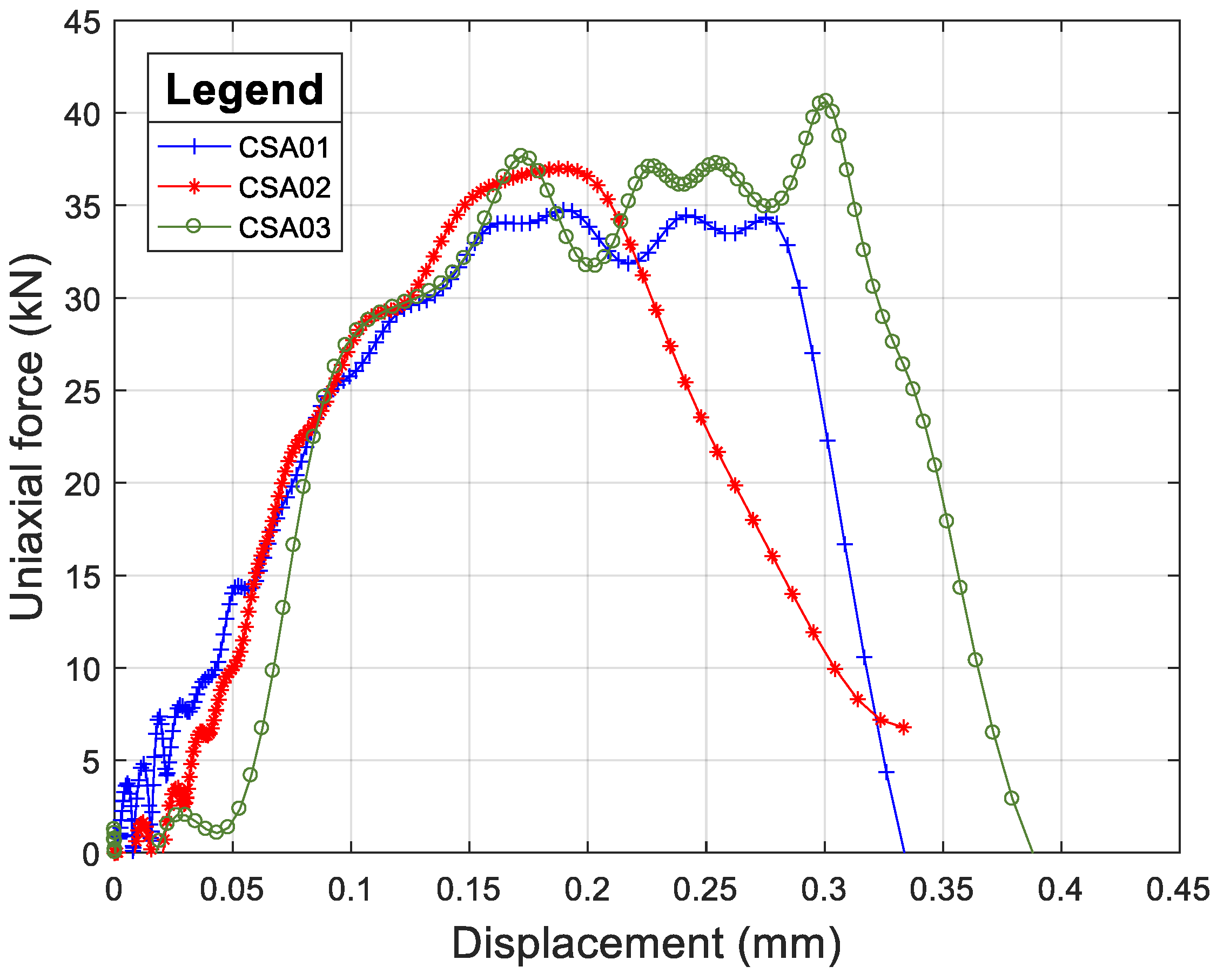
The graph shown in Figure 11 corresponds to the post-processing of the total force (average of input and output forces) with the deformation (difference of input and output displacements) obtained by the SHPB method as given by Equation (3), and processed using the DAVID software as described in [27].
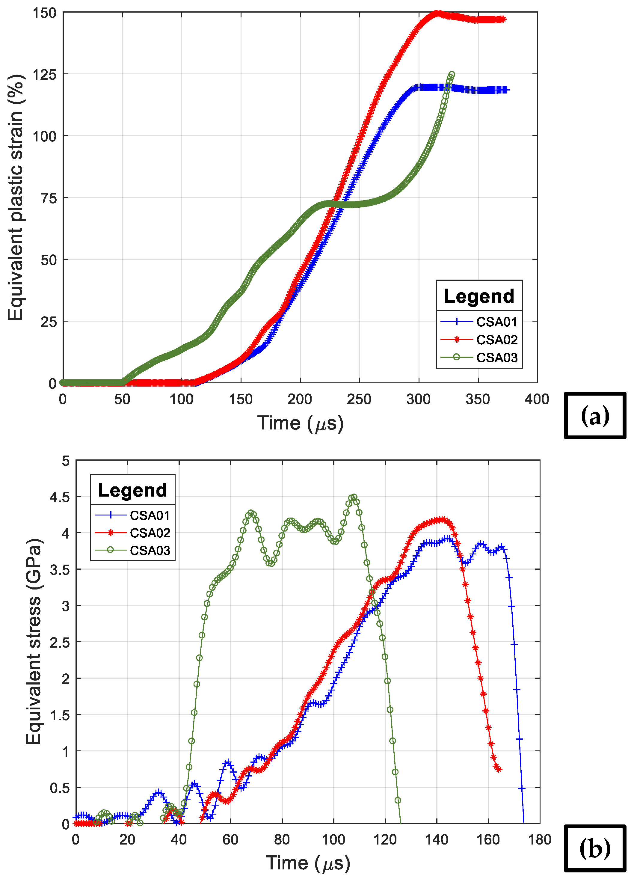
The equivalent plastic strain versus time and equivalent stress versus time calculated from Equations (1) are plotted in the Figure 12a,b, respectively. The main difference between the CSA03 sample and the CSA01 and CSA02 samples was that no pulse-shaper was used with the CSA03 test. This explains the larger oscillations associated with the CSA03 test data.
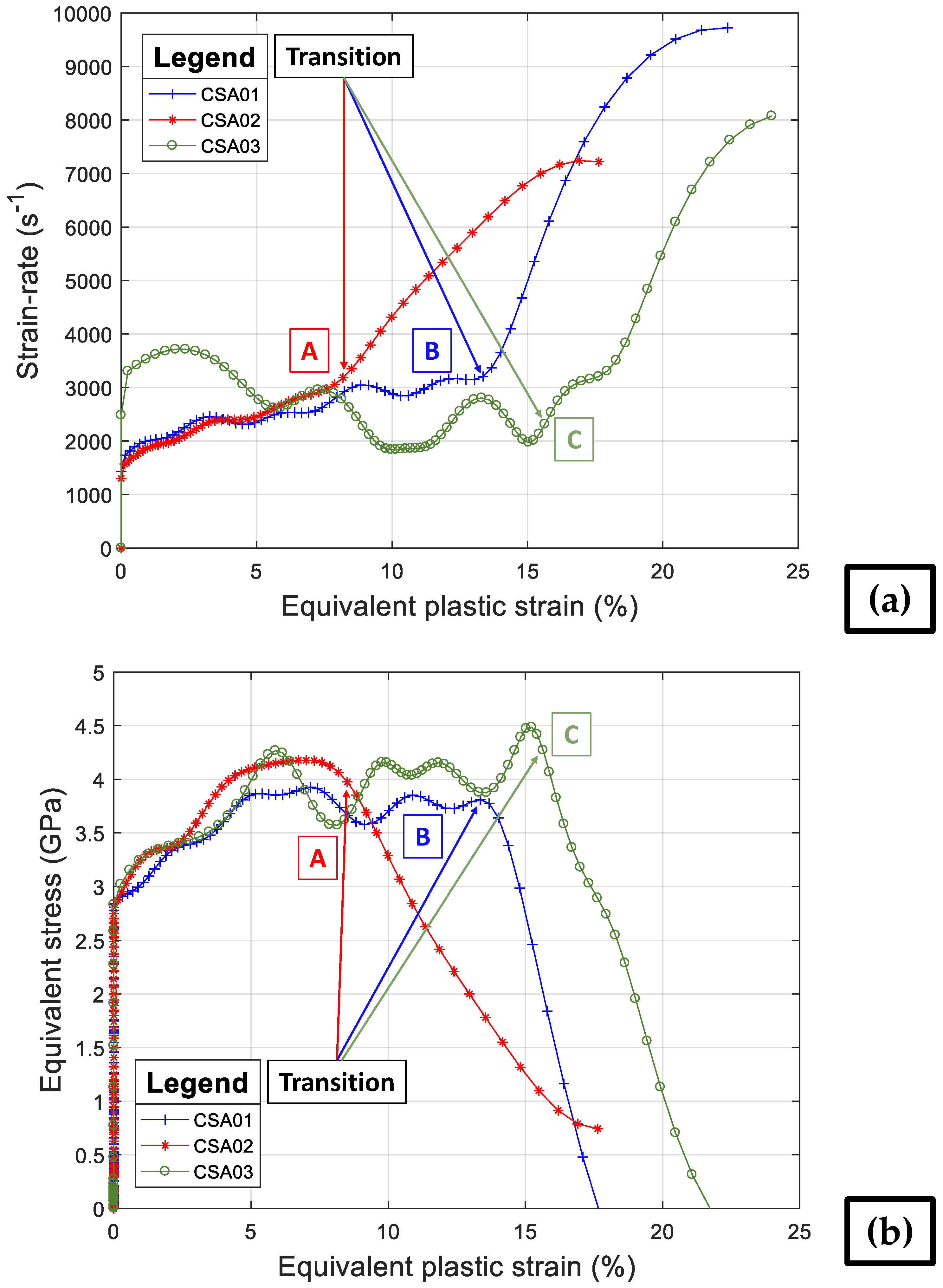
The elastic limit obtained from the dynamic tests for an equivalent plastic strain of 0.2% was evaluated as 3.0 GPa. If one considers 2% of equivalent plastic strain, the yield stress was about 3.4 GPa. The evolution of the strain-rate is illustrated in Figure 13a, and was shown to vary from 1000 at the beginning of the experiment to 3000 s−1 when a plastic strain of 8 to 15% was attained. Next, from the transition points depicted on Figure 13a, the strain-rate strongly increased, supposedly due to thermal softening: at high strain-rates, the plastic work induced a local increase of temperature (adiabatic heating) leading to a lowering of the material strength [28]. Finally, the stress-strain curves are plotted in Figure 13b after the experimental data were modified. The plastic plateau was reached for a plastic strain close to 5%. According to Figure 13a, at that time, the strain-rate is about 2,500 s−1 in all of the three samples.
Numerous regions of plastic deformation seem to appear on the fracture surface, Figure 14a (macro lens). In Figure 14b, optical microscopic pictures were obtained on unpolished samples using an EFI (Extended Focus Image) integrated algorithm enabling to see details beyond only one focus. The fracture surfaces of both samples tested under quasi-static and dynamic conditions appear quite rough and are characterised by small bright zones oriented along the direction of the notch. To better understand the state stress at failure in the ligament, the fields of normal stress and shear stress were represented considering the notch frame (i.e., the local frame compared to the global frame in ABAQUS, confer Appendix C). The numerical simulation (Figure 15) shows that the normal (axial) and tangential (shear) stresses are similar in amplitude. Finally, it is observed that the loading applied to the sheared region corresponds to a confined-shear loading involving high compressive normal stress along with the shear stresses.
4. Comparison between Quasi-Static and Dynamic Test Results
Shear-compression tests showed a weak sensitivity to strain-rate when comparing quasi-static and dynamic curves in Figure 16. The elastic limit (about 3.0 GPa) seems to be unchanged between the quasi-static and dynamic regimes. Only the flow stress appears to manifest a little sensitivity to the strain-rate. For an equivalent plastic strain of 5%, the equivalent stress is 3.7 GPa in the quasi-static regime whereas it is around 4.0 GPa in the dynamic regime (+8.1%). Considering the equivalent plastic strain at failure, the latter is lower in the dynamic regime; however, this is expected due to the loss of resistance of the metal due to adiabatic heating from plastic deformation.
Considering that the equivalent stress-plastic strain response significantly differs from the elastic-perfectly plastic behaviour assumed for the identification of ki parameters (Appendix A), a validation numerical test was considered as following:
- -
- The strain-hardening response was identified from “CS06 (QS)” test (Figure 16) and was introduced into an ABAQUS calculation.
- -
- A compression loading was applied to the numerical SCS sample considering a final displacement (0.4 mm, see Figure 9a).
- -
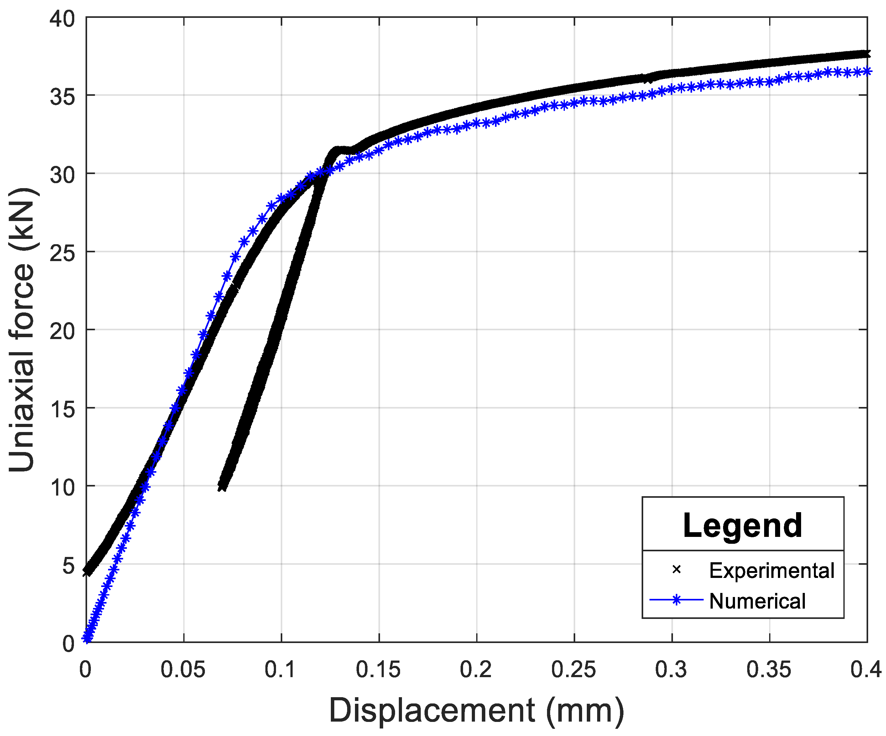
- The corresponding numerical force was extracted, and the force-displacement response was compared the experimental one (Figure 17).
It was observed that the numerical force matched with the experimental force until the sample breakage. At 0.4 mm, the relative difference between the numerical force (~36.5 kN) and the experimental force (~37.6 kN) was around 2.93%. Henceforth, it confirmed that the use of parameters (identified in Table 6) was consistent even in the present case involving a material presenting a moderate strain-hardening, as suggested in the validation of Section 3.2 (Figure 8).
5. Conclusions
The mechanical characterisation of very high strength steel used for the projectile core of AP projectiles was evaluated using SCS with a rectangular notch. The analysis was done by utilising a data processing method proposed in previous works. The processing parameters () for the SCS constitutive equations were determined using numerical simulations that assume an elastic-perfectly plastic constitutive behaviour of the numerical sample with an elastic limit close to the yield strength observed afterwards in the experiments. The accuracy of the processing method regarding a possible strain-hardening was evaluated by comparing the input constitutive law considered to model the sample’s behaviour to the output mechanical response obtained by processing the data of a strain-hardening constitutive model in numerical simulation. Next, both quasi-static and dynamic experiments were conducted using a load frame and a SHPB, respectively. The experimental forces and displacements were measured and processed using the previous methodology; therefore, the averaged equivalent plastic strain and equivalent stress in the sheared zone (ligament) were deduced. The quasi-static and dynamic tests showed a weak influence from strain-rate effects on the mechanical performance of this high strength steel. Additionally, this high strength steel exhibited a very high elastic limit of about 3.0 GPa with a small amount of strain-hardening before sudden failure. The identification of a constitutive law for the considered steel to be used in a numerical simulation of impact loading involving a 7.62 mm API-BZ projectile constitutes a natural prospect of this work.
Author Contributions
Conceptualisation: P.F.; Methodology: P.F., D.S., and Y.D.; Software: D.S., Validation: Y.D., D.S., and P.F.; Formal analysis: Y.D.; Investigation: Y.D., D.S., and P.F.; Resources: D.S. and P.F.; Writing – original draft: Y.D.; Writing—review & editing: Y.D., D.S., and P.F.; Visualisation: Y.D.; Supervision: D.S. and P.F.; Project administration: P.F.; Funding acquisition: P.F.
Funding
This research was funded by the DGA (Direction Générale de l’Armement) from the Ministry of the Armed Forces.
Acknowledgments
This research is part of Yannick Duplan’s PhD dissertation, and a project ordered and financed by the French MOD (Ministry Of Defence equivalent), in collaboration with the Saint-Gobain and Cedrem companies. For this reason, the authors want to thank the latter two for sponsoring this work. The authors also wish to thank the Cedrem company, who manufactured and supplied the samples used for testing.
Conflicts of Interest
The authors declare no conflict of interest.
Appendix A. Identification of Data Processing Parameters and Validation
Appendix A.1. Identification
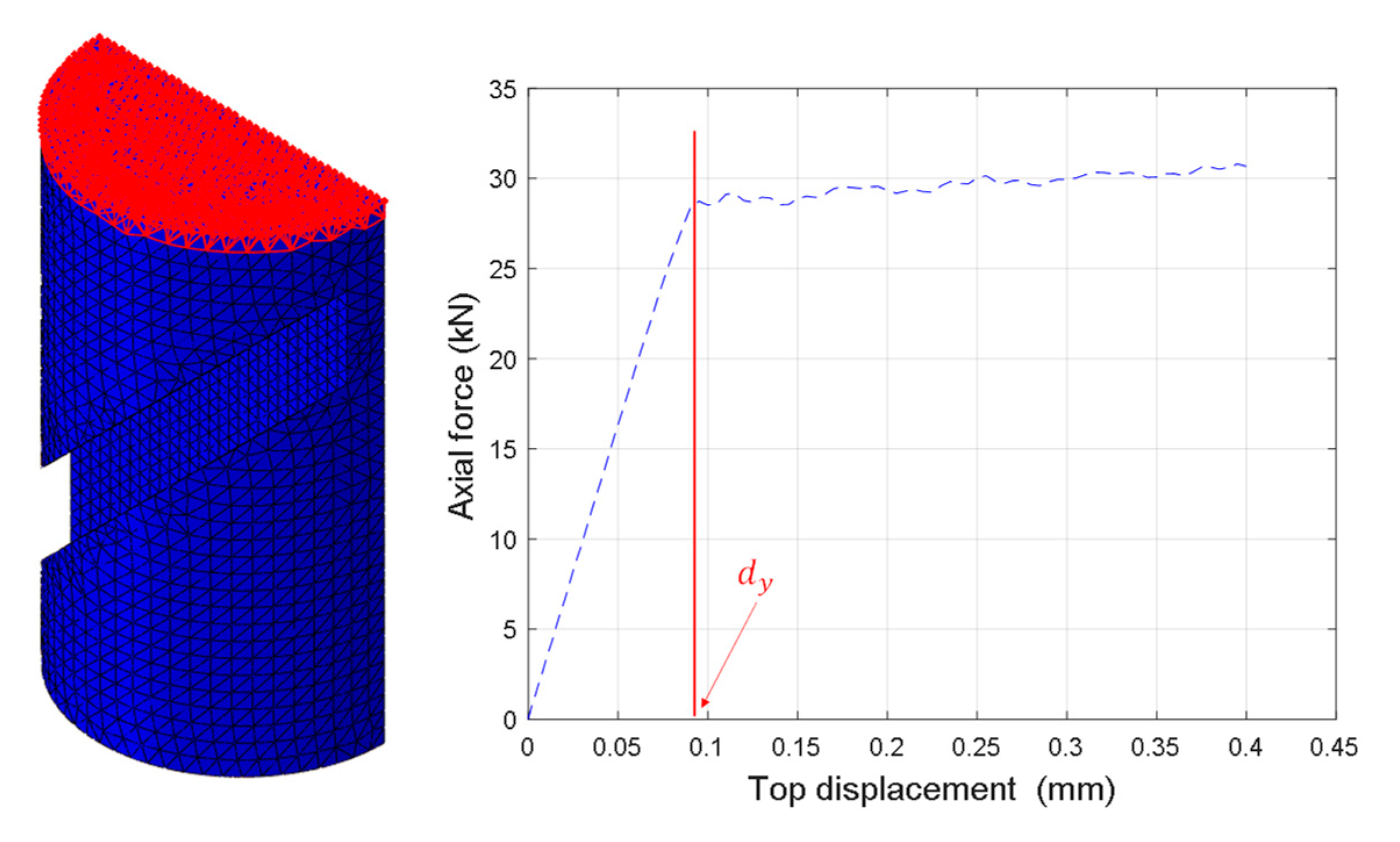
According to Equations (1), , , and are determined by first plotting the function . Here, is identified as the displacement corresponding to the elastic limit (the point where the linear force-displacement response as highlighted in Figure A1 is lost), and was equal to 8.969 × 10⁻⁵ m for the parameters given in the Table 2. The equivalent plastic strain (PEEQ variable in ABAQUS) corresponding to was averaged from the red elements ligament and was plotted as function of the total displacement in Figure A2. As expected, it can be concluded that starts increasing when the displacement is equal to .
Figure A1.
Identification of from the numerical (element nodal extraction in red) versus (unique nodal extraction) plot.
Figure A1.
Identification of from the numerical (element nodal extraction in red) versus (unique nodal extraction) plot.

Figure A2.
Evolution of the numerical value of in the notch section as a function of .

Based on this result, it can be concluded the functional form for can be obtained as shown by the results in Figure A3. A third order polynomial trend line that best fits the points (in the sense of least squares) was calculated to fit the equivalent plastic strain in Equation (1), where the intercept was forced to the origin, and then, , , and were identified. The power three was helpful when the curve was not linear. Here, was not needed but still retained to reach as much accuracy as possible.
Figure A3.
Evolution of as a function of the normalised plastic displacement.

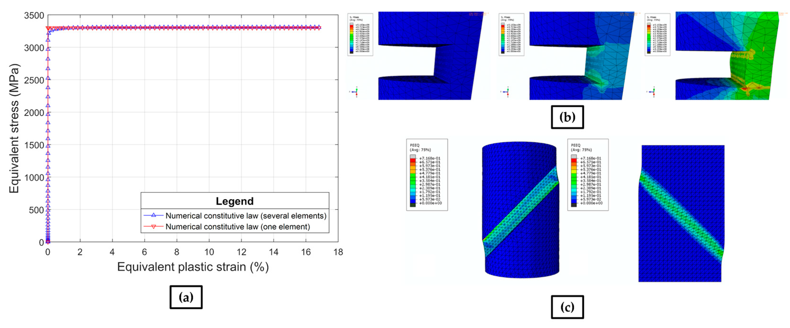
In addition, , , and were determined by plotting the equivalent (Huber-Mises) stress versus equivalent plastic strain as shown in Figure A4a. Here, the overall response converges to the constitutive law result. Additionally, the homogeneity of the plastic deformation was sparsely verified as shown in Figure A4b. From Figure A4c, it is observed that the plastic strain is concentrated within the notches of the sample.
Figure A4.
Numerical results for: (a) the equivalent Huber-Mises stress versus equivalent plastic strain, where one curve is being averaged in the ligament and the other one is the output of a single element; (b) the equivalent stress field in the notched section of the sample (t = 0 (left), 22 µs (middle), and 100 μs (right); (c) the equivalent plastic strain in the sample.

To identify the parameters and , the second equation in Equation (1) was rewritten in Equation (A1):
As reported by Francart et al. (2017) [21], the coefficient was set to 1. Thus, equation (A1) is a linear equation of the form , where and . The coefficients of this equation are and , and are calculated as illustrated in Figure A5.
Figure A5.
Identification of coefficients and with the curve obtained from equation (A1) starting at 0.9 on the y-axis.
Figure A5.
Identification of coefficients and with the curve obtained from equation (A1) starting at 0.9 on the y-axis.

Table 6 in Section 3.1 recalls each value of the coefficients .
Appendix A.2. Validation
The evaluation of the reliability of the parameters is presented below. Similarly to Section 3.2, the processing method was applied to the numerical force and numerical displacement . The variables and were compared with and . The comparison of these values from both methods is shown in Figure A6 and Figure A7, respectively.
Figure A6.
Comparison of with versus time obtained in the shear zone for numerical and processed data.
Figure A6.
Comparison of with versus time obtained in the shear zone for numerical and processed data.

Figure A7.
Comparison of with versus time obtained in the shear zone for numerical and processed data.
Figure A7.
Comparison of with versus time obtained in the shear zone for numerical and processed data.

Appendix B. Correction in QS Data
Direct measurement using LVDT’s needed to be corrected by taking into account the deformation of the plateaus and the parts of the machine in-between the sample and the LVDT supports due to the fact the tested samples were small and very rigid. This was accomplished by conducting an initial test with no sample and considering only the WC plugs. Therefore, the displacement was deduced, and a linear identification method was employed (). Next this function was utilized to correct the measured displacement as function of the applied force such that .
Appendix C. Calculation of Normal and Tangential Stress on the Notch System
Cauchy law (Equation (A2)) of the stress vector associated to the stress tensor of a normal :
Given the global frame () and the local frame of the notch () in Figure 15, and .
If ones defines the normal and the shear stresses:
The tensor is expressed in the () frame:
Thus, the normal and shear stresses become (A5):
The stress components of the Cauchy stress tensor correspond to in ABAQUS.
References
- den Reijer, P.C. Impact on Ceramic Faced Armours. Ph.D. Thesis, Technische Universiteit Delft, Delft, The Netherlands, 28 November 1991. [Google Scholar]
- Chen, X.W.; Chen, G.; Zhang, F.J. Deformation and failure modes of soft steel projectiles impacting harder steel targets at increasing velocity. Exp. Mech. 2008, 48, 335–354. [Google Scholar] [CrossRef]
- Normandia, M.; Lasalvia, J.; Gooch, W.; McCauley, J.W.; Rajendran, A.M. Protecting the future force: Ceramics research leads to improved armor performance. Amptiac Q 2004, 8, 21–27. [Google Scholar]
- Savio, S.G.; Senthil, P.; Singh, V.; Ghoshal, P.; Madhu, V.; Gogia, A.K. An experimental study on the projectile defeat mechanism of hard steel projectile against boron carbide tiles. Int. J. Impact Eng. 2015, 86, 157–166. [Google Scholar] [CrossRef]
- Tang, R.T.; Wen, H.M. Predicting the perforation of ceramic-faced light armors subjected to projectile impact. Int. J. Impact Eng. 2017, 102, 55–61. [Google Scholar] [CrossRef]
- Kılıç, N.; Bedir, S.; Erdik, A.; Ekici, B.; Taşdemirci, A.; Güden, M. Ballistic behavior of high hardness perforated armor plates against 7.62 mm armor piercing projectile. Mater. Des. 2014, 63, 427–438. [Google Scholar] [CrossRef]
- Fras, T.; Murzyn, A.; Pawlowski, P. Defeat mechanisms provided by slotted add-on bainitic plates against small-calibre 7.62 mm × 51 AP projectiles. Int. J. Impact Eng. 2017, 103, 241–253. [Google Scholar] [CrossRef]
- Kalthoff, J.F.; Bürgel, A. Influence of loading rate on shear fracture toughness for failure mode transition. Int. J. Impact Eng. 2004, 30, 957–971. [Google Scholar] [CrossRef]
- Xia, K.; Yao, W. Dynamic rock tests using split Hopkinson (Kolsky) bar system—A review. J. Rock Mech. Geotech. Eng. 2015, 7, 27–59. [Google Scholar] [CrossRef]
- Hundy, B.B.; Green, A.P. A determination of plastic stress-strain relations. J. Mech. Physcis Solids 1954, 3, 16–21. [Google Scholar] [CrossRef]
- Meyer, L.W.; Halle, T. Shear strength and shear failure, overview of testing and behavior of ductile metals. Mech. Time-Depend. Mater. 2011, 15, 327–340. [Google Scholar] [CrossRef]
- Cady, C.M.; Liu, C.; Trujillo, C.P.; Brown, D.W.; Gray III, G.T. The shear response of beryllium as a function of temperature and strain rate. EPJ Web Conf. 2018, 183, 02017. [Google Scholar] [CrossRef]
- Rittel, D.; Lee, S.; Ravichandran, G. A shear-compression specimen for large strain testing. Exp. Mech. 2002, 42, 58–64. [Google Scholar] [CrossRef]
- Dorogoy, A.; Rittel, D. Numerical validation of the shear compression specimen. Part I: Quasi-static large strain testing. Exp. Mech. 2005, 45, 167–177. [Google Scholar] [CrossRef]
- Dorogoy, A.; Rittel, D. Numerical validation of the shear compression specimen. Part II: Dynamic large strain testing. Exp. Mech. 2005, 45, 178–185. [Google Scholar] [CrossRef]
- Rittel, D.; Ravichandran, G.; Lee, S. Large strain constitutive behavior of OFHC copper over a wide range of strain rates using the shear compression specimen. Mech. Mater. 2002, 34, 627–642. [Google Scholar] [CrossRef]
- Dorogoy, A.; Rittel, D.; Godinger, A. Modification of the shear-compression specimen for large strain testing. Exp. Mech. 2015, 55, 1627–1639. [Google Scholar] [CrossRef]
- Dorogoy, A.; Rittel, D. Determination of the johnson–cook material parameters using the SCS specimen. Exp. Mech. 2009, 49, 881–885. [Google Scholar] [CrossRef]
- Bao, Y.; Wierzbicki, T. On fracture locus in the equivalent strain and stress triaxiality space. Int. J. Mech. Sci. 2004, 46, 81–98. [Google Scholar] [CrossRef]
- Francart, C. Experimental and numerical study of the mechanical behavior of metal/polymer multilayer composite for ballistic protection. Ph.D. Thesis, Université de Strasbourg, Strasbourg, France, 13 November 2017. [Google Scholar]
- Francart, C.; Demarty, Y.; Bahlouli, N.; Ahzi, S. Dynamic characterization and modeling of ductile failure of sintered aluminum alloy through shear-compression tests. Procedia Eng. 2017, 197, 69–78. [Google Scholar] [CrossRef]
- Rittel, D.; Wang, Z.G. Thermo-mechanical aspects of adiabatic shear failure of AM50 and Ti6Al4V alloys. Mech. Mater. 2008, 40, 629–635. [Google Scholar] [CrossRef]
- Abaqus Analysis User’s Guide (6.14)—28.1.1 Solid (Continuum) Elements. Available online: https://www.sharcnet.ca/Software/Abaqus/6.14.2/v6.14/books/usb/default.htm?startat=pt06ch28s01alm01.html (accessed on 21 January 2019).
- Hopkinson, B. A method of measuring the pressure produced in the detonation of high, explosives or by the impact of bullets. Philos. Trans. R. Soc. Lond. Ser. Contain. Pap. Math. Phys. Character 1914, 213, 437. [Google Scholar] [CrossRef]
- Kolsky, H. An investigation of the mechanical properties of materials at very high rates of loading. Proc. Phys. Soc. Sect. B 1949, 62, 676. [Google Scholar] [CrossRef]
- Dorogoy, A.; Rittel, D. Dynamic large strain characterization of tantalum using shear-compression and shear-tension testing. Mech. Mater. 2017, 112, 143–153. [Google Scholar] [CrossRef]
- Gary, G. DAVID, Instruction Manual; DAVID Group: Palaiseau, France, 2005. [Google Scholar]
- Meyers, M.A. Plastic Deformation at High Strain Rates. In Dynamic Behavior of Materials; John Wiley & Sons: New York, NY, USA, 1994; ISBN 978-0-471-58262-5. [Google Scholar]
Figure 1.
(a) Impact time history of a 7.62 mm APM2 projectile [3]; (b) post-test longitudinal cross-sectional view of a 7.62 mm Armour-Piercing (AP) projectile interacting with a boron carbide tile target (the black arrows indicate the shear bands) [4].

Figure 2.
Penetration/perforation sequences from numerical simulations of 7.62 × 54 mm AP projectiles striking base armour plates. (a) At the centre of a hole, (b) at the side of a hole [6].
Figure 2.
Penetration/perforation sequences from numerical simulations of 7.62 × 54 mm AP projectiles striking base armour plates. (a) At the centre of a hole, (b) at the side of a hole [6].

Figure 3.
The shear compression specimen (SCS) geometry used in the present work (dimensions in mm).
Figure 3.
The shear compression specimen (SCS) geometry used in the present work (dimensions in mm).

Figure 4.
7.62 mm API-BZ projectile and core.

Figure 5.
Cycles and loading conditions for quasi-static compressed samples.

Figure 6.
Experimentally measured input and output forces at the sample/bars interfaces in three dynamic experiments.
Figure 6.
Experimentally measured input and output forces at the sample/bars interfaces in three dynamic experiments.

Figure 7.
Comparison of quantities () averaged in the ligament of a numerical simulation involving a sample with strain-hardening to the quantities () obtained by applying the processing method to the numerical force and displacement extracted from the numerical simulation. On the left part, the processing method is based on parameters (Table 8). On the right part, the processing method is based on parameters of Table 6.

Figure 8.
Comparison of numerical () response averaged in the ligament of a numerical simulation involving a sample with strain-hardening to the () response obtained by applying the processing method to the numerical force and displacement extracted from the numerical simulation. Left: use of parameters (Table 8), Right: use of parameters (Table 6).

Figure 9.
(a) Recorded quasi-static data for the CS06 sample (with grease); (b) equivalent stress versus equivalent plastic strain curves for two quasi-static tests.
Figure 9.
(a) Recorded quasi-static data for the CS06 sample (with grease); (b) equivalent stress versus equivalent plastic strain curves for two quasi-static tests.

Figure 10.
Post-test photographs of samples subjected to quasi-static SCS experiments. Test with grease (CS06): a single inclined fracture plane is noted. Test without grease (CS07): the fracture surface is composed of two inclined planes.
Figure 10.
Post-test photographs of samples subjected to quasi-static SCS experiments. Test with grease (CS06): a single inclined fracture plane is noted. Test without grease (CS07): the fracture surface is composed of two inclined planes.

Figure 11.
Uniaxial force vs differential displacement response for tests CSA01, CSA02, and CSA03.

Figure 12.
(a) Temporal evolution of the dynamic equivalent plastic strain for three dynamic tests. (b) Temporal evolution of equivalent stress for three dynamic tests.
Figure 12.
(a) Temporal evolution of the dynamic equivalent plastic strain for three dynamic tests. (b) Temporal evolution of equivalent stress for three dynamic tests.

Figure 13.
(a) Strain-rate as a function of the equivalent plastic strain for three dynamic tests, with transition points between plastic flow and failure. (b) Equivalent stress versus equivalent plastic strain curves for three dynamic tests.
Figure 13.
(a) Strain-rate as a function of the equivalent plastic strain for three dynamic tests, with transition points between plastic flow and failure. (b) Equivalent stress versus equivalent plastic strain curves for three dynamic tests.

Figure 14.
(a) Closer view on the notch section of a dynamic-loaded sample (CSA02), ×10 macro lens. (b) Fractographies of notch surfaces, ×5 lens magnification.
Figure 14.
(a) Closer view on the notch section of a dynamic-loaded sample (CSA02), ×10 macro lens. (b) Fractographies of notch surfaces, ×5 lens magnification.

Figure 15.
Comparison stresses in the global frame and plot of the normal and shear stresses in the local frame of the notch.
Figure 15.
Comparison stresses in the global frame and plot of the normal and shear stresses in the local frame of the notch.

Figure 16.
Equivalent stress versus equivalent plastic strain response: comparison of quasi-static and dynamic tests.
Figure 16.
Equivalent stress versus equivalent plastic strain response: comparison of quasi-static and dynamic tests.

Figure 17.
Comparison between the experimental force-displacement response of test (CS06) to the numerical response of a sample modelled with the constitutive law that corresponds to the behaviour identified in the present work.
Figure 17.
Comparison between the experimental force-displacement response of test (CS06) to the numerical response of a sample modelled with the constitutive law that corresponds to the behaviour identified in the present work.


Table 1.
Chemical composition of API-BZ steel nuance.
| Chemical Element (Symbol) | Composition (wt %.) |
|---|---|
| Steel (Fe) | 97.4 |
| Carbon (C)/Sulphur (S) | 1.160/0.008 |
| Silicon (Si) | 0.25 |
| Chromium (Cr) | 0.23 |
| Nickel (Ni) | 0.23 |
Table 2.
Material parameters used in the numerical simulation.
| Parameter | Value |
|---|---|
| Physical parameter | |
| Density (Kg·m−3) | 7785 |
| Mechanical parameter–Elastic (supposed for a steel) | |
| Young’s modulus (GPa) | 210 |
| Poisson’s ratio | 0.3 |
| Mechanical parameter–Perfectly plastic (no strain hardening) | |
| Elastic limit (GPa) | 3.3 |
Table 3.
Sample dimensions and interface conditions.
| Id | Height H (mm) | Diameter D (mm) | Distance between Notches τ (mm) | Interface Conditions |
|---|---|---|---|---|
| CS06 | 9.92 | 6.01 | 1.45 | With grease |
| CS07 | 9.84 | 6.04 | 1.46 | Without grease |
Table 4.
Dimensions of the split Hopkinson pressure bar (SHPB) system.
| Identification | Length (mm) | Diameter (mm) |
|---|---|---|
| Striker bar | 450 | 20 |
| Input bar | 1500 | 20 |
| Output bar | 1200 | 20 |
Table 5.
Sample dimensions (dynamic case).
| Id | Height H (mm) | Diameter D (mm) | Distance between Notches τ (mm) |
|---|---|---|---|
| CSA01 | 9.94 | 6.06 | 1.40 |
| CSA02 | 9.94 | 6.05 | 1.42 |
| CSA03 | 9.98 | 6.06 | 1.41 |
Table 6.
Values of and parameters used for data processing of SCS (identification considering no strain-hardening).
Table 6.
Values of and parameters used for data processing of SCS (identification considering no strain-hardening).
| 1.2155 | |
| −0.0539 | |
| −0.9752 | |
| 0.9671 | |
| 0.2679 | |
| 1.0000 | |
| (mm) | 0.08969 |
Table 7.
Material strain-hardening parameters (close to the experimental response of the material) used instead of the concerned model in Table 2.
Table 7.
Material strain-hardening parameters (close to the experimental response of the material) used instead of the concerned model in Table 2.
| Parameter | Value |
|---|---|
| Mechanical parameter—Yield stress with strain hardening | |
| Yield stress (GPa)|Plastic strain | 2.7|0 |
| 3.3|0.1 | |
| 3.9|0.2 | |
Table 8.
Values of and parameters used for data processing of SCS (identification considering the strain-hardening of Table 7.
Table 8.
Values of and parameters used for data processing of SCS (identification considering the strain-hardening of Table 7.
| 1.0391 | |
| −1.5654 | |
| 2.3236 | |
| 0.9613 | |
| 0.2802 | |
| 1.0000 | |
| (mm) | 0.07632 |
© 2019 by the authors. Licensee MDPI, Basel, Switzerland. This article is an open access article distributed under the terms and conditions of the Creative Commons Attribution (CC BY) license (http://creativecommons.org/licenses/by/4.0/).
Share and Cite
MDPI and ACS Style
Duplan, Y.; Saletti, D.; Forquin, P. Identification of the Quasi-Static and Dynamic Behaviour of Projectile-Core Steel by Using Shear-Compression Specimens. Metals 2019, 9, 216. https://doi.org/10.3390/met9020216
AMA Style
Duplan Y, Saletti D, Forquin P. Identification of the Quasi-Static and Dynamic Behaviour of Projectile-Core Steel by Using Shear-Compression Specimens. Metals. 2019; 9(2):216. https://doi.org/10.3390/met9020216
Chicago/Turabian StyleDuplan, Yannick, Dominique Saletti, and Pascal Forquin. 2019. "Identification of the Quasi-Static and Dynamic Behaviour of Projectile-Core Steel by Using Shear-Compression Specimens" Metals 9, no. 2: 216. https://doi.org/10.3390/met9020216
Note that from the first issue of 2016, this journal uses article numbers instead of page numbers. See further details here.