Applying Machine Learning to the Phenomenological Flow Stress Modeling of TNM-B1


1
Chair of Mechanical Design and Manufacturing, Brandenburg University of Technology Cottbus-Senftenberg, Konrad-Wachsmann-Allee 17, D-03046 Cottbus, Germany
2
Department of Metallurgy and Materials Technology, Brandenburg University of Technology Cottbus-Senftenberg, Konrad-Wachsmann-Allee 17, D-03046 Cottbus, Germany
*
Author to whom correspondence should be addressed.
Metals 2019, 9(2), 220; https://doi.org/10.3390/met9020220
Submission received: 23 November 2018
/
Revised: 19 January 2019
/
Accepted: 29 January 2019
/
Published: 13 February 2019
(This article belongs to the Special Issue Constitutive Modelling for Metals)
Abstract
:Data-driven or machine learning approaches are increasingly being used in material science and research. Specifically, machine learning has been implemented in the fields of materials discovery, prediction of phase diagrams and material modelling. In this work, the application of machine learning to the traditional phenomenological flow stress modelling of the titanium aluminide (TiAl) alloy TNM-B1 (Ti-43.5Al-4Nb-1Mo-0.1B) is investigated. Three model types were developed, analyzed and compared; a physics-based phenomenological model (PM) originally developed for steel by Cingara and McQueen, a purely data-driven machine learning model (MLM), and a hybrid model (HM), which uses characteristic points predicted by a learning algorithm as input for the phenomenological model. The same amount of data was used to both fit the PM and train the MLM and HM. The models were analyzed and compared based on the accuracy of their predictions, development and computing time, and their ability to predict on interpolated and extrapolated inputs. The results revealed that for the same amount of experimental data, the MLM was more accurate than the PM. In addition, the MLM was better able to capture the characteristic peak stress in the TNM-B1 the flow curves, and could be developed and computed faster. Furthermore, the MLM was able to make realistic predictions for inputs outside the experimental data used for training. The HM showed comparable accuracy to the PM for the experimental conditions. However, the HM was able to produce a better fit for input conditions outside the training data.
1. Introduction
The task of predicting material behavior for a given process is essential in material science and engineering. Traditionally, this task has been carried out using physics-based mathematical modeling. However, the development of such models require both knowledge of the underlying physical phenomena and extensive amounts of experimental data. Alternatively, the data could be used for a data-driven or machine learning (ML) approach to modeling. A pure ML model requires no knowledge of the laws governing material behavior as it can learn a mapping function, which connects process input to outputs based purely on the examples from experimental data. In the past decade, ML has made many contributions to society. Self-driving cars, speech recognition and internet search recommendations are all the results of the continual improvements to computational power and learning algorithms. In material science, machine learning based models are promising due to the availability of experimental data in the field, and they have already been employed to enhance and accelerate several areas of research. These include prediction of phase diagrams, material properties and behavior, and the discovery and design of new materials based on existing databases such as stress-strain data and chemical composition data [1,2,3].
This work focuses on modeling the flow stress of the titanium aluminide (TiAl) alloy TNM-B1 (Ti-43.5Al-4Nb-1Mo-0.1B) during hot forging. This is an attractive material to the aerospace, automotive, power generation and related industries due to its high strength to weight ratio and high resistance to heat, corrosion and creep. Specifically, hot forged TiAl turbine blades have seen implementation in commercial jet engines [4]. In general, TiAl material models describing hot deformation behavior are empirical and phenomenological models that were originally derived for steels and adapted to TiAl [5,6,7,8]. As steel is commonly hot worked in the austenitic phase, these models were designed to model single-phase materials. In contrast, TiAl alloys have a complex multi-phase microstructure with various microstructural features. The material model investigated in this work is based on a phenomenological model developed for 300 austenitic steels and published by Cingara and McQueen [9]. This model was previously adapted to TiAl and evaluated in an earlier work by the authors [10]. In short, characteristic points on the experimental flow curves are extracted from the data and used to fit the model equations through regression analysis. This is called phenomenological modeling, as it is based on the observations of a phenomena rather than being derived from fundamental theory. Although the model has displayed high accuracy in predicting the flow curves for TiAl, the model equations do not account for the reorientation of lamellar colonies, flow localization and recrystallization of all the individual phases, all of which strongly influence the behavior of TiAl during deformation [11].
The deformation behavior of TNM-B1 during forging is dependent on a wide range of interconnected processes; work hardening, softening, dynamic recrystallization, dynamic recovery and generation of heat can all occur simultaneously and influence each other. In addition, the behavior varies with process temperature, applied force and speed. As there is a knowledge gap in understanding the complete deformation behavior from the macroscopic scale to the atomic scale, deformation processes such as hot forging can be difficult to handle using physics-based modeling. In addition, developing and computing such models can be time consuming. Previous studies have explored the application of pure machine learning as well as hybrid approaches to material modeling. Lin et al. utilized an artificial neural network (ANN) to predict the flow stress behavior of a 42CrMo steel during hot compression [12]. The ANN was trained on temperature, strain and strain rate data to learn a mapping function that could output flow stress. The authors used the performance indicator ’average absolute relative error’ (AARE), and achieved an error of around 4.5 % when testing the ANN on new data not used for training the network. Zhu et al. developed a hybrid model consisting of a combination of neuro-fuzzy and physics-based models [13]. The aim was to predict flow stress and microstructure evolution during thermomechanical processing of aluminum-magnesium alloys. The hybrid model was integrated into a finite element simulation, which gave very similar results as compared to empirical models. Yu et al. used a fuzzy neural network (FNN) in order to predict ultimate tensile strength, yield strength, elongation and area reduction of Ti-6Al-4V based on forging temperature, strain and strain rate [14]. The FNN used a neural network to find the parameters of a fuzzy rule set. It was verified that the model could predict mechanical properties, which could aid in practical optimization of processing parameters. Sheikh et al. employed two parallel ANN models to predict the flow stress of a 5083 aluminum alloy, in regions of serrated flow and smooth yielding respectively, during tensile testing at room temperature and elevated temperatures [15]. The experimental temperature, strain and strain rate data were used as training inputs to learn a mapping function that outputs flow stress. The results showed good agreement between the experimental data and predicted values for all conditions.
The literature includes studies on the use of neural networks and hybrid approaches to predict the behavior of steels and other materials including TiAl alloys. However, no such study exists for TNM-B1. In addition, the development of a hybrid model combining machine learning with a traditional phenomenological model is absent in the literature. In this study, three different approaches to modeling the flow stress behavior of TNM-B1 are explored and compared; a phenomenological model (PM) for TiAl adapted from a model originally developed for steel by Cingara and McQueen, a pure machine learning model (MLM), consisting of a neural network trained to predict the entire flow stress curve as a function of temperature, strain and strain rate, and finally a hybrid model (HM), consisting of two parallel neural networks trained to predict the position of the characteristic points on the experimental flow curves as functions of temperature and strain rate, which were then used as input for the phenomenological model to predict the final flow curves. For this purpose, hot compression tests were performed to extract experimental flow stress data. The tests were conducted at the temperatures 1150, 1175 and 1200 °C, and the strain rates 0.0013, 0.005, 0.01 and 0.05 s−1. The same amount of experimental data was used to fit the PM, and to train the MLM and the HM. The models were analyzed and compared based on the accuracy of their predictions, efficiency in terms of development and computing time, and their ability to produce accurate predictions on interpolated and extrapolated inputs between and outside the experimental data.
2. Materials and Methods
2.1. Material and Microscopy
The investigated TNM-B1 alloy, with the composition given in Table 1, was produced using vacuum arc remelting (VAR) by GfE Metalle und Materialien GmbH (Nürnberg, Germany). The material was subsequently hot isostatically pressed (HIPed) to close microporosities, using the parameters 1200 °C, 200 MPa and 4 h. This produced an ingot with a height of 150 mm and a diameter of 49 mm, which was eroded into cylinders with a height of 95 mm and a diameter of 7 mm. This was done using electrical discharge machining (EDM) by Erocontur GmbH (Müncheberg, Germany). Finally, the cylinders were cut and turned into test samples with a height of 8 mm and a diameter of 5 mm.
The microscopy images of the TNM-B1 sample were taken with a TESCAN Mira II (Brno, Czech Republic) scanning electron microscope (SEM), using the back-scattered electron (BSE) mode with an acceleration voltage of 14.5 kV. Prior to imaging, the sample surface was grinded with a RotoPol-22 from Struers (Berlin, Germany), using a speed of 300 rpm and a force of 20 N. SiC grinding paper with a gradation ranging from 240 to 2500 was used. After grinding, the samples were polished for 72 h in a VibroMet 2 from Buehler (Uzwil, Switzerland). The samples were suspended in distilled water and Collodial Silica from LECO Corp. (St. Joseph, MO, USA).
2.2. Compression Tests
The hot compression tests were performed using a DIL805A/D/T quenching and deformation dilatometer from TA Instruments (New Castle, DE, USA), former Bähr Thermoanalyse GmbH (Germany). Molybdenum plates with a thickness of around 1 mm were placed between the specimen and the Si3N4-punches in the dilatometer. The tests were conducted in an argon atmosphere to protect from oxidation. The cylindrical samples were isothermally deformed using the following parameters; the constant strain rates 0.0013 s−1, 0.005 s−1, 0.01 s−1 and 0.05 s−1, and the constant temperatures 1150 °C, 1175 °C and 1200 °C. The strain rate of 0.0013 s−1 was used as this was the lowest strain rate allowed by the test equipment. The sample and molybdenum plates were first heated by induction using a heating rate of 10 K/s, and held at the testing temperature for 3 min to obtain a homogeneous microstructure and quasi-isothermal conditions prior to deformation. The samples were deformed from 0 to around 0.8 strain. Finally, the samples were cooled at a rate of 200 K/s using argon gas. The experiments were duplicated at least two times to ensure repeatability in the resulting flow curves.
2.3. Phenomenological Model Fundamentals
The phenomenological material model (PM) used in this work was developed and published by Cingara and McQueen [9]. The model equations are summarized in Table 2. It uses separate dynamic recrystallization (DRX) kinetics for the and phases, as different parameters are used to model these two phases.
For modeling TiAl, the main feature of this model is the ability to show a concave course in the strain-hardening rate in the so-called Kocks-Mecking plot, as can be observed experimentally. This is a plot of the strain hardening rate () as a function of flow stress . Other models that are derived from dislocation theory are not applicable to TiAl alloys, as they cannot reproduce a concave curvature in the Kocks-Mecking plot. An overview of various dislocation-based models is presented in [10]. The basic concept behind the present model is that characteristic points extracted from the flow curve can be expressed as a function of the Zener-Hollomon parameter (Table 2). These characteristic points are used to fit the model parameters to the experimental data using regression analysis. The model contains an equation for strain hardening (SH) and dynamic recovery (DRV) of the non-recrystallized material, an initiation criterion for DRX, an equation for the recrystallized grain size, an equation for DRX kinetics and a mixture rule to determine the macroscopic flow stress when recrystallized and non-recrystallized grains coexist.
Figure 1 illustrates the modelled flow curve due to SH and DRV, and the adjusted flow curve with softening due to DRX kinetics included (other phenomena can also contribute to the softening behavior). In addition, the positions of the characteristic points are shown; peak stress/strain (), critical stress/strain () and steady state stress/strain (). The peak stress is the maximum stress reached. The steady state stress is the point at which steady state deformation is reached. The location of the steady state strain strongly influences the shape of the modelled flow curve. As true steady state of TNM-B1 is not always achieved during a hot deformation test, the value has to be assumed and can thus be a source of error. The critical strain marks the onset of dynamic recrystallization (DRX). In steels, this point can be extracted from the inflection point in the Kocks-Mecking plot [16]. However, TiAl alloys shows no such inflection point. Therefore, the critical strain and stress of TNM-B1 could not be determined from stress-strain data alone. In this work, the critical strain was calculated by setting to 0.5 from experience [10].
2.4. Machine Learning Model Fundamentals
The aim of the pure machine learning model (MLM) was to train a learning algorithm to predict the flow stress of TNM-B1 during isothermal deformation as a function of temperature, strain rate and strain. The models developed in this work were trained on the principle of supervised learning, where both the inputs and the intended outputs are known variables and an algorithm attempts to learn a mapping function between the two. The machine learning framework used was the artificial neural network (ANN). This section briefly covers the principles and terminology used for ANNs, see [17,18] for further reading. Artificial neural networks are inspired by biological neural networks, and attempt to replicate the way humans learn and process information. They consist of interconnected artificial neurons or processing elements organized in layers; an input layer, an output layer and hidden layers in between, as illustrated in Figure 2a. The ANN is referred to as shallow if it has one hidden layer and deep (i.e., deep learning) if the number of hidden layers exceeds one.
Each layer of the ANN consists of a number of artificial neurons, as illustrated in Figure 2b. In short, an artificial neuron receives inputs from the original input data or other nodes in an earlier hidden layer, and computes an output. This is done by calculating a weighted sum of its inputs and adding a bias, where the weights and the biases are the parameters to be learned. An activation function is then applied to decide if the neuron should fire or not (i.e., pass along its output to other neurons). Equation (1a) describes how the inputs are handled within the neuron.
where are the weights, are the inputs and b is the bias. This sum is then passed through an activation function, which is typically a sigmoid function (Equation (1b). Here, the sum is translated to a number between 0 and 1. If this number is above a certain threshold, the neuron fires. The purpose of the activation function is to introduce non-linearity to the neuron output, as most real world data is non-linear. This process of passing the input data through the neurons of the neural network is called feed forward. After one feed forward, the resulting output of the network is compared to the known intended output from data via a cost function. In this work, the mean squared error (MSE) cost function was used (Equation (2)).
where is the known intended output, is the prediction made by the neural network and n is the number of data points. An optimization algorithm then attempts to minimize the cost function, in order to improve the performance of the ANN (i.e., to predict values closer to the intended output), by going backwards through the ANN and manipulating the weights and biases in a process called back propagation. In this work, the Levenberg–Marquardt optimization algorithm was utilized. This is a widely used non-linear least squares fitting algorithm first proposed by Kenneth Levenberg and later improved by Donald Marquardt [19,20]. One cycle of feed forward and back propagation is called an epoch. In theory, each completed epoch increases the network performance. In practice, diminishing returns, overfitting (i.e., fitting to the noise in the input data) or increases in the cost function can occur. As such, it is important to stop the evolution of the network at the epoch of highest performance.
Data cleaning is one of the most important and time-consuming parts of developing a machine learning model, as the quality of the data used for training the model strongly impacts the predictive power of the final model. However, automating the process becomes possible once the methods to cleaning the specific data are known. The data used to train a neural network is commonly split into three subsets; a training set, a test set and a validation set. The training set is a dataset of examples used for learning the relationship between the inputs and the intended output. In other words, it is used to adjust and optimize the ANN parameters (i.e., weights and biases) during training. However, if this optimization runs unchecked, the network will transition from modeling the underlying behavior of the data into modeling the noise in the data (i.e., overfitting). For this reason, a separate validation set not used for training the network is used. If the prediction accuracy compared to the training set increases, but the accuracy compared to the “unseen” validation set decreases, the network is most likely being overfitted and training should be stopped. This is commonly called early stopping. Usually, the criterion for early stopping is an increase in the validation error beyond a set threshold with an increasing number of epochs. The test set is used for testing the final network in order to assess its performance.
2.5. Hybrid Model Fundamentals
The aim of the hybrid model (HM) was to replace the equations of the phenomenological model that model the dependence on the characteristic points with machine learning, by training ANNs (described in Section 2.4) to predict the position of the characteristic points (critical, peak, steady state stress and strain) as functions of temperature and strain rate (illustrated in Figure 3). These predicted values were used as input for the phenomenological model (described in Section 2.3), which subsequently produced the final flow curves.
3. Results and Discussion
3.1. Microstructure Overview and Deformation Behavior
The microstructure of TNM-B1 consists of lamellar colonies and globular structures, as displayed in Figure 4. TNM-B1 consists of the ordered phases -TiAl (dark contrast), -Ti3Al (gray contrast) and -TiAl (bright contrast), all of which have different individual deformation behaviors [21,22]. The phase has a hexagonal close-packed (HCP) structure, with the highest strength and lowest formability in the TNM-B1 system. The phase has a face-centered cubic (FCC) crystal structure, with higher strength than the phase, but higher deformability than the phase. The phase has a body-centered cubic (BCC) A2 structure, and the phase has a body-centered cubic (BCC) B2 structure. At high temperatures, it is the softest phase of the TNM-B1 alloy [23]. Therefore, the phase carries a much higher strain during hot deformation than the nominal value, leading to highly misoriented subgrains and dynamic recrystallization (DRX). In general, the macroscopic deformation behavior of TNM-B1 is strongly dependant on DRX, dynamic recovery (DRV) and the orientation of the lamellar colonies.
The compression test results revealed variations in the measured flow stresses for the same conditions. This is a problem inherent to TiAl, and is thought to be partly due to the randomly distributed initial orientation and reorientation of lamellar colonies during deformation. Previous studies have demonstrated that the ductility and strength of TiAl are sensitive to the orientation of lamellar colonies with respect to the loading axis [24,25]. As the + lamellar colonies of TNM-B1 possesses low deformability relative to the surrounding globular and cellular and grains, they are to a larger extend reoriented into more favorable orientations rather than being deformed during the early stages of deformation. The optimal orientation is when the lamellar boundaries are parallel to the loading axis [26]. Thus, the ratio of favorably to unfavorably oriented lamellar colonies in the initial undeformed microstructure can strongly influence the deformation behavior of TNM-B1, and can lead to varied results between tests for the same conditions. Several tests were conducted for each temperature and strain rate in order to obtain two similar flow curves. The highest variance in peak stress was around 25 MPa at 1150 °C and 0.01 s−1.
3.2. Phenomenological Model Results
In this section, the results of the phenomenological model (PM) are presented and discussed. The characteristic points (peak stress/strain, critical stress/strain and steady state stress/strain) were extracted from the experimental flow curves obtained for TNM-B1, and used as input for the PM as described in Section 2.3. The experimental flow curves and the flow curves predicted by the PM are displayed in Figure 5. As is characteristic for TiAl, the experimental flow curves of TNM-B1 show an initial steep rise in stress up to a pronounced peak, followed by a strong softening behavior until steady state deformation. True steady state was not reached in all tests (discussed in Section 2.3). The results revealed that the PM predicted a generalized flow curve shape for all conditions. This can lead to fairly accurate predictions, as can be seen in the flow curves obtained for 0.0013 and 0.05 s−1. However, the PM was not able to capture the characteristic sharp peak for some conditions, which can be observed especially in the flow curves obtained for 0.01 s−1.
To assess and compare the accuracy of the predicted flow curves, the mean squared error (MSE) was used as a performance indicator. The PM achieved an MSE of around 16.3, which is equivalent to an average error of around 4 MPa between the experimental stress values and the predicted ones. The highest error made by the PM was around 33.1 MPa, and was made near the peak stress of the flow curve at 1150 °C and 0.01 s−1. The computing time for generating the flow curves was 17.9 s. The error histogram for the PM is displayed in Figure 6, which shows the error distribution in MPa.
3.3. Machine Learning Model Results
In this section, the results of the pure machine learning model (MLM) are presented and discussed. Artificial neural networks (ANN), which are described in Section 2.4, were trained on the experimental flow curve data obtained for TNM-B1. The aim was to learn a mapping function that outputs a predicted flow stress based on the inputs temperature, strain rate and strain. The process of developing the MLM consisted of three main steps; data cleaning, adjusting hyperparameters (i.e., the number of hidden layers and neurons) to find the optimal ANN architecture, and evaluating the final model performance.
First, the experimental data was cleaned. Due to physical factors, small variations existed in the data. The average of the measured temperature and strain rate vectors were close to the initial experimental settings, and were thus replaced with constant values. The measured strain and stress vectors were kept unchanged. This was done to prevent overfitting to small variations in the temperature and strain rate data, and promote fitting between strain and stress. In addition, the relatively big variations in flow stress between tests conducted at the same conditions can lead to the ANN learning strong local dependencies on the small variations in temperature and strain rate. In other words, it can learn that the small variations in temperature and strain rate are the cause for the difference in flow stress, and predict unrealistic relationships. Table 3 displays the cleaned dataset used for training the MLM. The first three rows and the last row are shown. In total, 103,296 rows of training examples from 24 flow curves for different conditions were used.
Prior to each ANN training session, the experimental data was randomly split into three subsets, as discussed in Section 2.4. A standard split of 70 % training data, 15 % test data and 15 % validation data was chosen. Figure 7 illustrates an early accuracy evolution of the different subsets in an example training session, where the optimal validation set MSE only reached 30.4 (equivalent to 5.5 MPa) at epoch 26. This network was not used to produce results. After epoch 26, the training and test error decreased, and the validation error increased. As this increase in validation error reached a certain threshold, early stopping was initiated as overfitting beyond this point was assumed. Thus, the training session was concluded and the network parameters (i.e., weights and biases) obtained at epoch 26 were extracted and saved, as this network produced the lowest validation MSE before overfitting occurred. Note that the accuracy evolution shown varies for each ANN training session.
To identify the optimal network architecture for the TNM-B1 flow curve data, the hyperparameters were tuned iteratively through a process of trial and error. Several architectures ranging from shallow to deep were tested. Table 4 displays a selection of the tested architectures to illustrate the process. 10 tests were conducted on each architecture, and each architecture was trained for 1000 epochs or until early stopping occurred. The averages of the number of hidden layers (HL), number of neurons (N), the minimum mean squared error achieved (MSE) with the equivalent stress, training time and standard deviations are shown. As both the data split and the initial weights and biases are randomly chosen at the beginning of training, each trained ANN converged at different network parameters, giving different MSE scores and predicted values. The training times also varied greatly, as some networks were stopped early and some continued making incremental accuracy improvements for the entire 1000 epoch limit. The best MSE scores achieved with the shallow networks were around 12 to 16, and only the training time increased with increasing complexity. The deepest networks tested achieved similar MSE scores to less complex networks, with increased training times. It was found that the optimal architecture in terms of both accuracy and training time for the ANN was 2 hidden layers with 10 neurons in the first layer and 3 neurons in the second layer. The best performing ANN of this architecture achieved an MSE of 6.7 with a training time of around 1 minute and 44 s, and was used to produce the predicted flow curves shown in Figure 8.
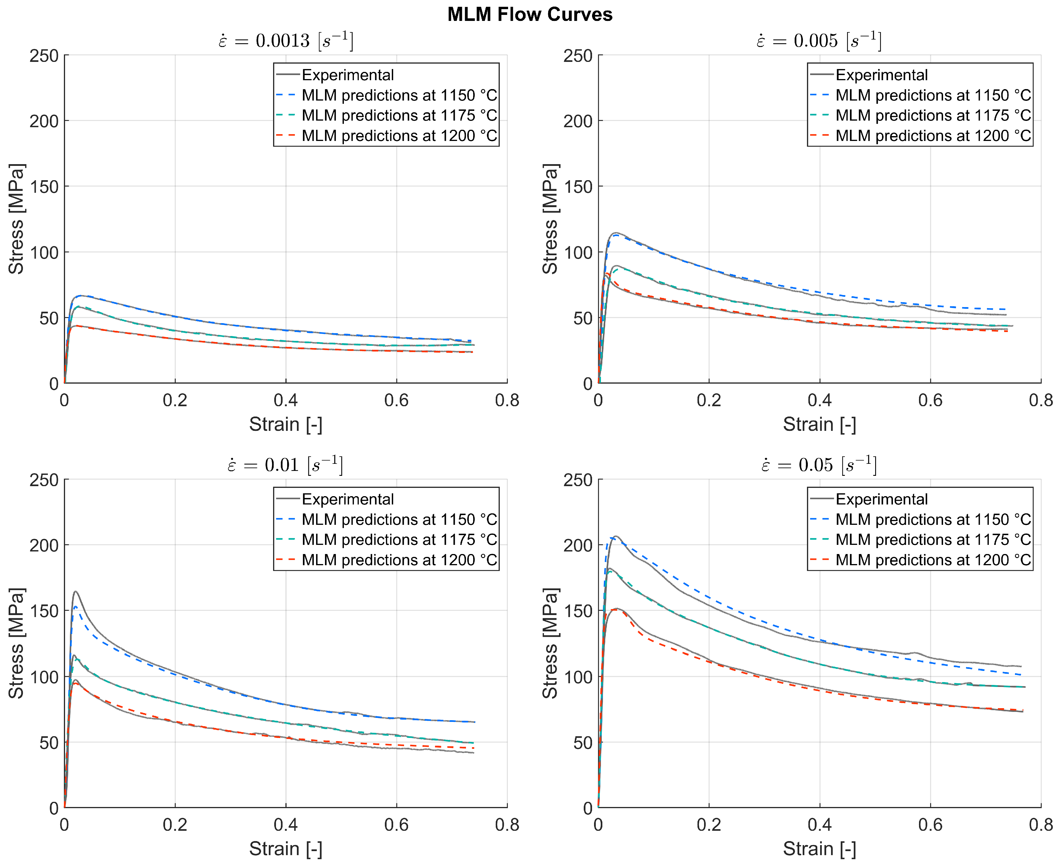
The experimental flow curves and the flow curves predicted by the best performing MLM are displayed in Figure 8. The MSE score achieved of 6.7 is equivalent to an average error of around 2.6 MPa in predicted flow stress. The highest error made was around 27.1 MPa in the elastic region of the flow curve at 1150 °C and 0.05 s−1, due to the MLM predicting a slightly steeper rise in stress than the experimental curve. The computing time for running the data through the finished ANN to predict the flow stress was around 0.06 s. The results reveal that the MLM was able to capture the sharp peak stress of the TNM-B1 flow curve, while avoiding overfitting to the noise in the data. In addition, the MLM is observed to adapt to the different flow curve shapes rather than outputting a generalized shape for every input condition. Figure 9 displays the error histogram for the MLM, with the errors given in MPa. By comparing this to the error histogram of the PM (Figure 6), it is apparent that the MLM predicts more values closer to zero error than the PM.
3.4. Hybrid Model Results
In this section, the results of the hybrid model (HM) are presented and discussed. The HM is described in Section 2.5. The ANNs were trained on the characteristic points (Figure 1) extracted from the experimental flow curve data of TNM-B1. The aim was to learn mapping functions, which uses the inputs temperature and strain rate to output the position of the characteristic points. To improve performance, two parallel ANNs were trained. One was trained on the characteristic strain values (Table 5), and the other on the characteristic stress values (Table 6). The first three rows and the last row of the datasets are shown. In total, 72 rows of data from 24 flow curves were used for each ANN.
Using the same process of trial and error as described in Section 3.3, the hyperparameters were tuned in order to find the optimal network architecture. It was found that a network consisting of 2 hidden layers with 10 neurons in the first layer and 5 neurons in the second layer was optimal for both MSE score and training time. The achieved MSE varied significantly for each training session. This was probably due to the limited amount of training examples, as only three characteristic points can be extracted from each flow curve. The best performing ANNs for predicting the characteristic stress and strain achieved respective MSE scores of around 30.4 (equivalent to an average stress error of around 5.5 MPa) and 6.3 × 10⁻⁵ (equivalent to an average strain error of around 0.008). The training times were in the order of 0.1 to 0.2 seconds. The predicted positions of the characteristic points were then used as input for the phenomenological model, which produced the final flow curves.
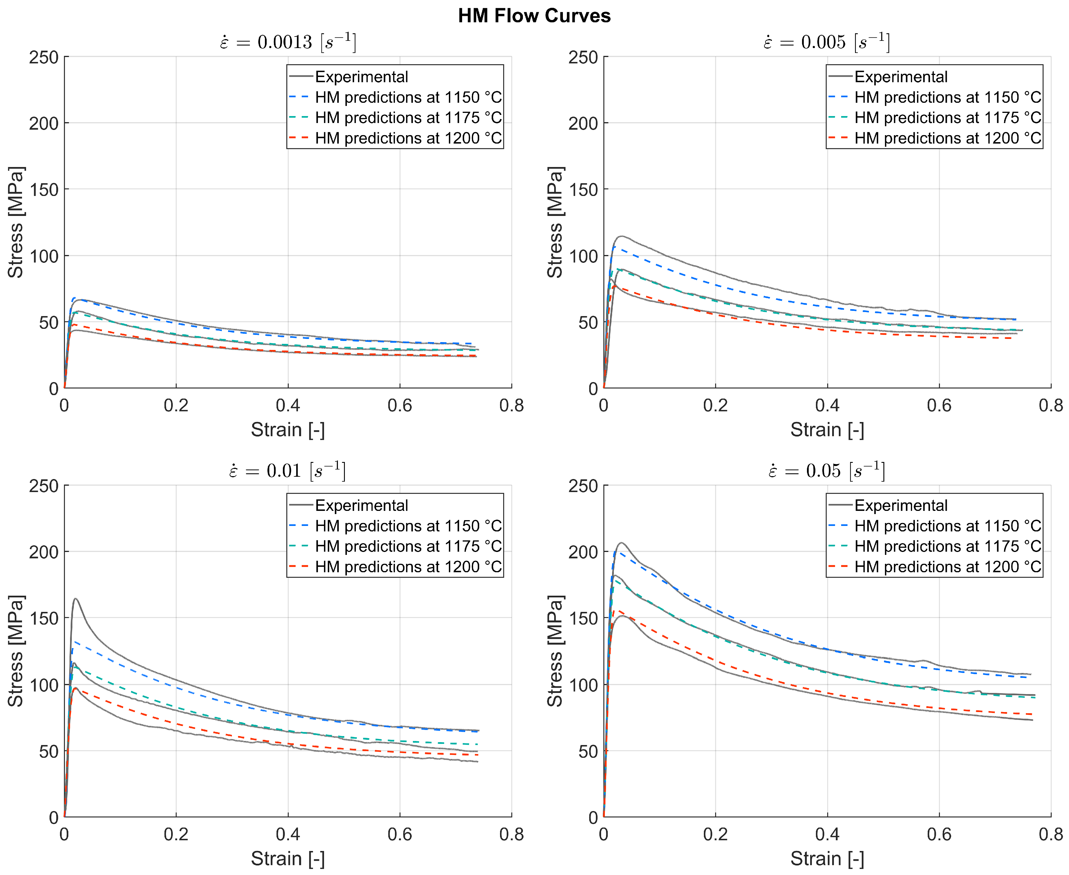
The experimental flow curves and the flow curves predicted by the HM are displayed in Figure 10. The HM flow curves were very similar to the PM ones, as the PM is a deterministic model and the predicted characteristic points were close to the experimental ones. The highest error made by the HM was around 33.1 MPa and was again made around the peak stress of the flow curve at 1150 °C and 0.01 s−1. The computing time for running the data through the finished ANNs to predict the characteristic stresses and strains was in the order of 0.05 s, and the computing time for generating the flow curves using the phenomenological model was 17.9 s. Figure 11 displays the error histogram for the HM, with the errors given in MPa.
3.5. Extrapolation and Interpolation
In this section, the ability of the PM, MLM and HM to make predictions on extrapolated and interpolated inputs is investigated. Figure 12, Figure 13 and Figure 14 display surface plots of the flow stresses predicted by the three different models for a range of temperature and strain rate inputs. In (a), the temperature was varied between 1125 and 1225 °C with an increment of 5 °C, at a constant strain rate of 0.0013 s−1. In (b), the strain rate was varied between 0.0005 and 0.1 s−1 with 10 increments between each power, at a constant temperature of 1150 °C. The line plots on the surface illustrate the flow curves predicted at the experimental conditions used for training the models. The line plots at the edges are experimental flow curves obtained to evaluate the ability of the models to make extrapolated predictions, this data was not used for training the ANNs or as input for the PM. As 0.0013 s−1 was the lowest strain rate allowed by the experimental setup (discussed in Section 2.2), flow stress data for 0.0005 s−1 could not be obtained. Figure 12 displays the ability of the PM to give stress predictions on interpolated and extrapolated inputs. The PM appears to produce conservative predictions at both lower temperatures and higher strain rates. The PM produced a smooth surface of predictions for the interpolated and extrapolated inputs.
Figure 13 illustrates the ability of the MLM to produce stress predictions on interpolated and extrapolated inputs. The plots shown were produced by the MLM iteration which gave the smoothest and most realistic surfaces in the set of 20 iterations displayed in Figure 15. As can be seen in Figure 13a, the extrapolated predictions at 1125 and 1225 °C correspond well with the experimental curves, with the surface being slightly jagged outside the experimental values. In Figure 13b, the predicted peak stress at 0.1 s−1 is around 50 MPa higher than the experimental peak of 253.6 MPa. However, the surfaces of predicted stress values as a whole corresponds well with what can be expected from real experimental data.
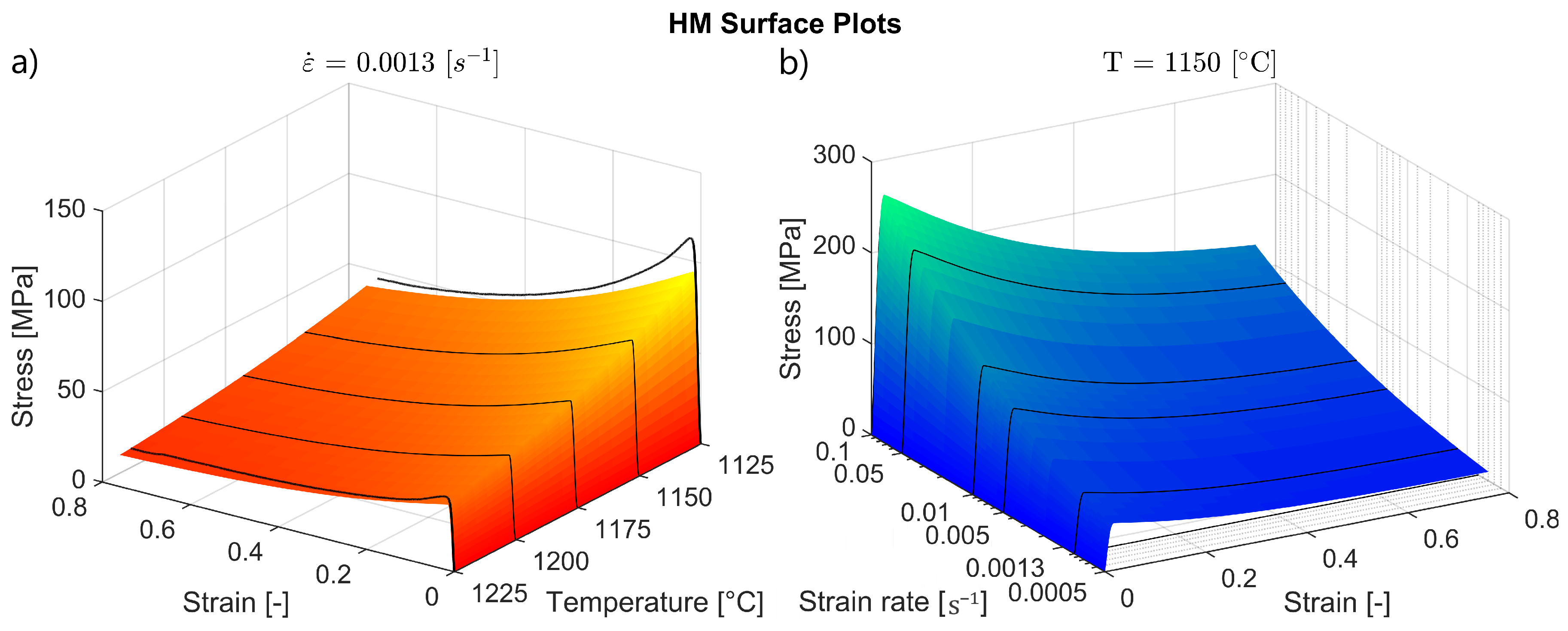
Two parallel ANNs trained on the characteristic points extracted from the flow curves, as described in Section 3.4, were used to make predictions for interpolated and extrapolated inputs. The predictions were then used as input for the phenomenological model to produce the surface plots displayed in Figure 14. The results revealed that the HM offers a better fit than the PM for both varied temperature and strain rate inputs, as the predicted stresses for extrapolated inputs better corresponds with the experimental flow curves. Comparing the HM to the MLM, the results are not as clear. The HM offers a better fit for varied strain rate inputs. However, the HM and the MLM offer similar results for varied temperature inputs.
As can be seen in Figure 8, the MLM can predict flow curves that correspond very closely with the experimental flow curves used for training. However, for temperature, strain and strain rate conditions outside the experimental inputs, the predicted stress values were often highly unrealistic. Figure 15 displays a cross section of the predicted stresses taken at 0.5 strain from 20 iterations of the MLM, with temperature inputs varying between 1125 and 1225 °C (a) and strain rate inputs varying between 0.0005 and 0.1 s−1 (b). While the networks produced very accurate predictions for the input data they were trained on, around half produced unrealistic predictions for inputs outside and between the training inputs. This suggests that although the MLM can give good predictions for the conditions used for training, its ability to extrapolate and interpolate varies significantly between training sessions and has to be verified. The probability that the MLM will learn a mapping function that produces realistic predictions for extrapolated and interpolated inputs is likely to increase with an increasing amount of training data.
4. Conclusions
In this work, the application of machine learning to the phenomenological flow stress modelling of the TiAl alloy TNM-B1 (Ti-43.5Al-4Nb-1Mo-0.1B) was investigated. Three different modeling approaches were studied; a phenomenological model (PM) for TiAl adapted from a model originally developed for steel by Cingara and McQueen [9], a pure machine learning model (MLM), consisting of a neural network trained to predict the entire course of the flow stress curves as a function of temperature, strain and strain rate, and finally a hybrid model (HM), consisting of two parallel ANNs trained to predict the position of characteristic points on the TNM-B1 flow curve as functions of temperature and strain rate, which were subsequently used as input for the phenomenological model to output the final flow curves. Hot compression tests were performed at the temperatures 1150, 1175 and 1200 °C, and the strain rates 0.0013, 0.005, 0.01 and 0.05 s−1, to extract the experimental flow stress data. The three models were analyzed and compared based on the accuracy of their predictions, efficiency and their ability to produce accurate predictions on interpolated and extrapolated input data. The main conclusions drawn from this investigation are:
- Using the same amount of experimental data, the MLM made more accurate predictions than the PM. In addition, the MLM was more efficient in terms of both development and computing time. The MLM was also better able to capture distinct features of the TNM-B1 flow curves, such as the characteristic sharp peak stress. These findings indicate that the equations modeling the course of the flow curve in the PM can be replaced by a pure machine learning approach.
- The MLM was able to produce predictions for extrapolated and interpolated inputs that gave a smooth and realistic fit, and which was comparable to what can be expected from experimental data. However, many training iterations were required due to the random elements of generating neural networks.
- The HM was able to produce a better fit compared to the PM for extrapolated and interpolated inputs. This indicates that the traditional PM can be improved by replacing the equations used to model the dependence on the characteristic points with machine learning.
Author Contributions
J.A.S. and M.B. conceived the work, J.A.S. performed the coding, modeling and wrote the paper, M.E. performed the microstructure analysis, I.S. performed the hot compression tests, M.B. and S.W. contributed with corrections.
Funding
This research has been funded by the Deutsche Forschungsgemeinschaft (DFG, German Research Foundation) through the projects WE 2671/7-1 and BA 4253/4-1.
Conflicts of Interest
The authors declare no conflict of interest.
Abbreviations
The following abbreviations are used in this manuscript:
| HIP | Hot Isostatic Pressing |
| TNM | TiAl with Nb and Mo as the main alloying elements |
| ANN | Articifial Neural Network |
| DRX | Dynamic Recrystallization |
| DRV | Dynamic Recovery |
| VAR | Vacuum Arc Remelting |
References
- Mueller, T.; Kusne, A.G.; Ramprasad, R. Machine learning in materials science: recent progress and emerging applications. Rev. Comput. Chem. 2016, 29, 186–273. [Google Scholar]
- Pilania, G.; Wang, C.; Jiang, X.; Rajasekaran, S.; Ramprasad, R. Accelerating materials property predictions using machine learning. Sci. Rep. 2013, 3, 2810. [Google Scholar] [CrossRef] [PubMed]
- Liu, Y.; Zhao, T.; Ju, W.; Shi, S. Materials discovery and design using machine learning. J. Mater. 2017, 3, 159–177. [Google Scholar] [CrossRef]
- Clemens, H.; Smarsly, W. Light-weight Intermetallic Titanium Aluminides—Status of Research and Development. Adv. Mater. Res. 2011, 78, 551–556. [Google Scholar] [CrossRef]
- Cheng, L.; Xue, X.; Tang, B.; Kou, H.; Li, J. Flow characteristics and constitutive modeling for elevated temperature deformation of a high Nb containing TiAl alloy. Intermetallics 2014, 49, 23–28. [Google Scholar] [CrossRef]
- Godor, F.; Werner, R.; Lindemann, J.; Clemens, H.; Mayer, S. Characterization of the high temperature deformation behavior of two intermetallic TiAl–Mo alloys. Mater. Sci. Eng. A 2015, 648, 208–216. [Google Scholar] [CrossRef]
- He, X.; Yu, Z.; Liu, G.; Wang, W.; Lai, X. Mathematical modeling for high temperature flow behavior of as-cast Ti–45Al–8.5Nb–(W,B,Y) alloy. Mater. Des. 2009, 30, 166–169. [Google Scholar] [CrossRef]
- Deng, T.Q.; Ye, L.; Sun, H.F.; Hu, L.X.; Yuan, S.J. Development of flow stress model for hot deformation of Ti-47%Al alloy. Trans. Nonferrous Met. Soc. China 2011, 21, 308–314. [Google Scholar] [CrossRef]
- Cingara, A.; McQueen, H.J. New formula for calculating flow curves from high temperature constitutive data for 300 austenitic steels. J. Mater. Proc. Technol. 1992, 36, 31–42. [Google Scholar] [CrossRef]
- Bambach, M.; Sizova, I.; Bolz, S.; Weiß, S. Devising Strain Hardening Models Using Kocks–Mecking Plots—A Comparison of Model Development for Titanium Aluminides and Case Hardening Steel. Metals 2016, 6, 204. [Google Scholar] [CrossRef]
- Appel, F.; Paul, J.D.H.; Oehring, M. Gamma Titanium Aluminide Alloys: Science and Technology; John Wiley & Sons: Hoboken, NJ, USA, 2011. [Google Scholar]
- Lin, Y.C.; Zhang, J.; Zhong, J. Application of neural networks to predict the elevated temperature flow behavior of a low alloy steel. Comput. Mater. Sci. 2008, 43, 752–758. [Google Scholar] [CrossRef]
- Zhu, Q.; Abbod, M.F.; Talamantes-Silva, J.; Sellars, C.M.; Linkens, D.A.; Beynon, J.H. Hybrid modelling of aluminium–magnesium alloys during thermomechanical processing in terms of physically-based, neuro-fuzzy and finite element models. Acta Mater. 2003, 51, 5051–5062. [Google Scholar] [CrossRef]
- Yu, W.; Li, M.Q.; Luo, J.; Su, S.; Li, C. Prediction of the mechanical properties of the post-forged Ti–6Al–4V alloy using fuzzy neural network. Mater. Des. 2010, 31, 3282–3288. [Google Scholar] [CrossRef]
- Sheikh, H.; Serajzadeh, S. Estimation of flow stress behavior of AA5083 using artificial neural networks with regard to dynamic strain ageing effect. J. Mater. Process. Technol. 2008, 196, 115–119. [Google Scholar] [CrossRef]
- Jonas, J.J.; Quelennec, X.; Jiang, L.; Martin, E. The Avrami kinetics of dynamic recrystallization. Acta Mater. 2009, 57, 2748–2756. [Google Scholar] [CrossRef]
- Anderson, J.A. An Introduction to Neural Networks. In A Bradford Book; The MIT Press: Cambridge, MA, USA, 1995. [Google Scholar]
- Rojas, R. Neural Networks: A Systematic Introduction; Springer: Berlin/Heidelberg, Germany, 1996. [Google Scholar]
- Levenberg, K. A Method for the Solution of Certain Non-Linear Problems in Least Squares. Q. Appl. Math. 1944, 2, 164–168. [Google Scholar] [CrossRef]
- Marquardt, D. An Algorithm for Least-Squares Estimation of Nonlinear Parameters. SIAM J. Appl. Math. 1963, 11, 431–441. [Google Scholar] [CrossRef]
- Schloffer, M.; Iqbal, F.; Gabrisch, H.; Schwaighofer, E.; Schimansky, F.P.; Mayer, S.; Stark, A.; Lippmann, T.; Göken, M.; Pyczak, F.; et al. Microstructure development and hardness of a powder metallurgical multi phase γ-TiAl based alloy. Intermetallics 2012, 22, 231–240. [Google Scholar] [CrossRef] [Green Version]
- Masahashi, N.; Mizuhara, Y.; Matsuo, M.; Hanamura, T.; Kimura, M.; Hashimoto, K. High Temperature Behavior of Titanium-Aluminide Based Gamma Plus Beta Microduplex Alloy. ISIJ Int. 1991, 31, 728–737. [Google Scholar] [CrossRef]
- Liu, B.; Liu, Y.; Qiu, C.; Zhou, C.; Li, J.; Li, H.; He, Y. Design of low-cost titanium aluminide intermetallics. J. Alloys Compd. 2015, 650, 298–304. [Google Scholar] [CrossRef]
- Inui, H.; Kishida, K.; Misak, M.; Kobayashi, M.; Shirai, Y.; Yamaguchi, M. Temperature dependence of yield stress, tensile elongation and deformation structures in polysynthetically twinned crystals of Ti-Al. Philos. Mag. A 1995, 72, 1609–1631. [Google Scholar] [CrossRef]
- Nakano, T.; Biermann, H.; Riemer, M.; Mughrabi, H.; Nakai, Y.; Umakoshi, Y. Classification of γ-γ and γ-α2 lamellar boundaries on the basis of continuity of strains and slip-twinning planes in fatigued TiAl polysynthetically twinned crystals. Philos. Mag. A 2001, 81, 1447–1471. [Google Scholar] [CrossRef]
- Inui, H.; Oh, M.H.; Nakamura, A.; Yamaguchi, M. Room-temperature tensile deformation of polysynthetically twinned (PST) crystals of TiAl. Acta Metall. Mater. 1992, 40, 3095–3104. [Google Scholar] [CrossRef]
Figure 1.
Flow curve illustrating the characteristic points; peak stress/strain (), critical stress/strain () and steady state stress/strain (). The thin line represents the modelled flow curve due to strain hardening (SH) and dynamic recovery (DRV). The thick line represents the modelled flow curve with dynamic recrystallization (DRX) kinetics included.

Figure 2.
(a) ANN schematic with one hidden layer, (b) artificial neuron schematic.

Figure 3.
Schematic of the hybrid model (HM). ANNs was trained to predict the characteristic points (critical, peak, steady state stress and strain) as functions of temperature (T) and strain rate (). These predictions are used as input for the phenomenological model, which outputs the final flow curves.

Figure 4.
SEM image of undeformed HIPed TNM-B1 and hot formed TNM-B1 at 1150 °C and 0.005 s−1, consisting of the ordered phases -TiAl (dark contrast), -Ti3Al (gray contrast) and /-TiAl (bright contrast). The loading direction is along the y-axis.
Figure 4.
SEM image of undeformed HIPed TNM-B1 and hot formed TNM-B1 at 1150 °C and 0.005 s−1, consisting of the ordered phases -TiAl (dark contrast), -Ti3Al (gray contrast) and /-TiAl (bright contrast). The loading direction is along the y-axis.

Figure 5.
Experimental flow curves and the PM predictions for TNM-B1 at the temperatures 1150, 1175 and 1200 °C and the strain rates 0.0013, 0.005, 0.01 and 0.05 s−1.
Figure 5.
Experimental flow curves and the PM predictions for TNM-B1 at the temperatures 1150, 1175 and 1200 °C and the strain rates 0.0013, 0.005, 0.01 and 0.05 s−1.

Figure 6.
Error histogram for the PM with 30 bins and a bin width of around 2.2 MPa. The results displayed are the difference between the experimental and predicted stress values.
Figure 6.
Error histogram for the PM with 30 bins and a bin width of around 2.2 MPa. The results displayed are the difference between the experimental and predicted stress values.

Figure 7.
Example accuracy evolution of the training, validation and test datasets.

Figure 8.
Experimental flow curves and the MLM predictions for TNM-B1 at the temperatures 1150, 1175 and 1200 °C and the strain rates 0.0013, 0.005, 0.01 and 0.05 s−1.
Figure 8.
Experimental flow curves and the MLM predictions for TNM-B1 at the temperatures 1150, 1175 and 1200 °C and the strain rates 0.0013, 0.005, 0.01 and 0.05 s−1.

Figure 9.
Error histogram for the MLM with 30 bins and a bin width of around 1.8 MPa. The results displayed are the difference between the experimental and predicted stress values.
Figure 9.
Error histogram for the MLM with 30 bins and a bin width of around 1.8 MPa. The results displayed are the difference between the experimental and predicted stress values.

Figure 10.
Experimental flow curves and the HM predictions for TNM-B1 at the temperatures 1150, 1175 and 1200 °C and the strain rates 0.0013, 0.005, 0.01 and 0.05 s−1.
Figure 10.
Experimental flow curves and the HM predictions for TNM-B1 at the temperatures 1150, 1175 and 1200 °C and the strain rates 0.0013, 0.005, 0.01 and 0.05 s−1.

Figure 11.
Error histogram for the HM with 30 bins and a bin width of around 2.2 MPa. The results displayed are the difference between the experimental and predicted stress values.
Figure 11.
Error histogram for the HM with 30 bins and a bin width of around 2.2 MPa. The results displayed are the difference between the experimental and predicted stress values.

Figure 12.
Surface plots of stress values predicted by the PM for interpolated and extrapolated inputs; (a) temperatures between 1125 and 1225 °C with an increment of 5 °C; (b) strain rates between 0.0005 and 0.1 s−1 with 10 increments between each power.
Figure 12.
Surface plots of stress values predicted by the PM for interpolated and extrapolated inputs; (a) temperatures between 1125 and 1225 °C with an increment of 5 °C; (b) strain rates between 0.0005 and 0.1 s−1 with 10 increments between each power.

Figure 13.
Surface plots of stress values predicted by the MLM for interpolated and extrapolated inputs; (a) temperatures between 1125 and 1225 °C with an increment of 5 °C, (b) strain rates between 0.0005 and 0.1 s−1 with 10 increments between each power.
Figure 13.
Surface plots of stress values predicted by the MLM for interpolated and extrapolated inputs; (a) temperatures between 1125 and 1225 °C with an increment of 5 °C, (b) strain rates between 0.0005 and 0.1 s−1 with 10 increments between each power.

Figure 14.
Surface plots of stress values predicted by the HM for interpolated and extrapolated inputs; (a) temperatures between 1125 and 1225 °C with an increment of 5 °C, (b) strain rates between 0.0005 and 0.1 s−1 with 10 increments between each power.
Figure 14.
Surface plots of stress values predicted by the HM for interpolated and extrapolated inputs; (a) temperatures between 1125 and 1225 °C with an increment of 5 °C, (b) strain rates between 0.0005 and 0.1 s−1 with 10 increments between each power.

Figure 15.
Cross section of interpolated and extrapolated surface plots from 20 tests at 0.5 strain.
Figure 15.
Cross section of interpolated and extrapolated surface plots from 20 tests at 0.5 strain.


Table 1.
Composition of the TNM-B1 ingots as specified by GfE.
| Al | Nb | Mo | B | O | Fe | Ni | C | |
|---|---|---|---|---|---|---|---|---|
| at% | 43.7 | 4 | 1 | 0.1 | 0.161 | 0.027 | 0.008 | 0.038 |
| wt% | 28.65 | 9.15 | 2.36 | 0.026 | 0.063 | 0.037 | 0.012 | 0.011 |
Table 2.
Overview of the model equations used in the phenomenological model.
| Zener-Hollomon parameter | |
| Strain hardening | |
| Critical strain | |
| Peak strain | |
| steady state strain | |
| Peak stress | |
| steady state stress | |
| DRX grain size | |
| DRX kinetics | |
| Flow stress |
Table 3.
Dataset used for training the ANNs to predict the entire course of the flow curves for TNM-B1, with the first three rows and the last row shown. Training inputs; temperature, strain rate and strain. Target output; flow stress.
Table 3.
Dataset used for training the ANNs to predict the entire course of the flow curves for TNM-B1, with the first three rows and the last row shown. Training inputs; temperature, strain rate and strain. Target output; flow stress.
| Row | Temp. [°C] | Strain rate [s−1] | Strain [-] | Stress [MPa] |
|---|---|---|---|---|
| 1 | 1150 | 0.0013 | 0 | 0 |
| 2 | 1150 | 0.0013 | 0.000357 | 0.954 |
| 3 | 1150 | 0.0013 | 0.000439 | 1.067 |
| ... | ... | ... | ... | ... |
| 103,296 | 1200 | 0.05 | 0.771 | 74.739 |
Table 4.
Performance of a selection of tested ANN architectures showing the number of hidden layers (HL), number of neurons (N), average achieved MSE (mean squared error), equivalent error in MPa and training time. 10 tests were conducted for each architecture.
Table 4.
Performance of a selection of tested ANN architectures showing the number of hidden layers (HL), number of neurons (N), average achieved MSE (mean squared error), equivalent error in MPa and training time. 10 tests were conducted for each architecture.
| HL | N | MSE | STD | Eq. Stress [MPa] | Training Time [s] | STD |
|---|---|---|---|---|---|---|
| 1 | 5 | 172.3 | 43.3 | 13.0 | 47.0 | 20.45 |
| 1 | 10 | 98.0 | 70.8 | 7.5 | 228.6 | 98.0 |
| 1 | 20 | 14.1 | 1.5 | 3.8 | 254.6 | 137.6 |
| 2 | 10, 3 | 10.4 | 1.9 | 3.2 | 210.0 | 141.9 |
| 2 | 15, 3 | 11.6 | 1.4 | 3.4 | 383.4 | 135.6 |
| 2 | 15, 5 | 10.6 | 1.5 | 3.3 | 309.8 | 139.0 |
| 3 | 15, 5, 3 | 14.1 | 3.3 | 3.7 | 260.4 | 72.7 |
| 4 | 5, 5, 5, 5 | 12.1 | 0.8 | 3.5 | 400.8 | 161.2 |
Table 5.
Dataset used for training the ANNs to predict the position of the characteristic strains (peak, critical and steady state strain), with the first three rows and the last row shown. Training inputs; temperature, strain rate and parameter type. Target output; characteristic strain.
Table 5.
Dataset used for training the ANNs to predict the position of the characteristic strains (peak, critical and steady state strain), with the first three rows and the last row shown. Training inputs; temperature, strain rate and parameter type. Target output; characteristic strain.
| Row | Temp. [°C] | Strain Rate [s−1] | Type | Ch. Strain [-] |
|---|---|---|---|---|
| 1 | 1150 | 0.0013 | Peak strain | 0.0328 |
| 2 | 1150 | 0.0013 | Peak strain | 0.0301 |
| 3 | 1150 | 0.005 | Peak strain | 0.0344 |
| ... | ... | ... | ... | ... |
| 72 | 1200 | 0.05 | steady state strain | 0.7708 |
Table 6.
Dataset used for training the ANNs to predict the position of the characteristic stresses (peak, critical and steady state stress), with the first three rows and the last row shown. Training inputs; temperature, strain rate and parameter type. Target output; characteristic stress.
Table 6.
Dataset used for training the ANNs to predict the position of the characteristic stresses (peak, critical and steady state stress), with the first three rows and the last row shown. Training inputs; temperature, strain rate and parameter type. Target output; characteristic stress.
| Row | Temp. [°C] | Strain Rate [s−1] | Type | Ch. Stress [MPa] |
|---|---|---|---|---|
| 1 | 1150 | 0.0013 | Peak stress | 66.555 |
| 2 | 1150 | 0.0013 | Peak stress | 63.494 |
| 3 | 1150 | 0.005 | Peak stress | 114.557 |
| ... | ... | ... | ... | ... |
| 72 | 1200 | 0.05 | steady state stress | 74.612 |
© 2019 by the authors. Licensee MDPI, Basel, Switzerland. This article is an open access article distributed under the terms and conditions of the Creative Commons Attribution (CC BY) license (http://creativecommons.org/licenses/by/4.0/).
Share and Cite
MDPI and ACS Style
Stendal, J.A.; Bambach, M.; Eisentraut, M.; Sizova, I.; Weiß, S. Applying Machine Learning to the Phenomenological Flow Stress Modeling of TNM-B1. Metals 2019, 9, 220. https://doi.org/10.3390/met9020220
AMA Style
Stendal JA, Bambach M, Eisentraut M, Sizova I, Weiß S. Applying Machine Learning to the Phenomenological Flow Stress Modeling of TNM-B1. Metals. 2019; 9(2):220. https://doi.org/10.3390/met9020220
Chicago/Turabian StyleStendal, Johan A., Markus Bambach, Mark Eisentraut, Irina Sizova, and Sabine Weiß. 2019. "Applying Machine Learning to the Phenomenological Flow Stress Modeling of TNM-B1" Metals 9, no. 2: 220. https://doi.org/10.3390/met9020220
Note that from the first issue of 2016, this journal uses article numbers instead of page numbers. See further details here.