Avrami Kinetic-Based Constitutive Relationship for Armco-Type Pure Iron in Hot Deformation

Institute of Machinery Manufacturing Technology, Chinese Academy of Engineering Physics, Mianyang 621900, China
*
Author to whom correspondence should be addressed.
Metals 2019, 9(3), 365; https://doi.org/10.3390/met9030365
Submission received: 2 March 2019
/
Revised: 15 March 2019
/
Accepted: 16 March 2019
/
Published: 21 March 2019
(This article belongs to the Special Issue Constitutive Modelling for Metals)
Abstract
:The work presents a full mathematical description of the stress-strain compression curves in a wide range of strain rates and deformation temperatures for Armco-type pure iron. The constructed models are based on a dislocation structure evolution equation (in the case of dynamic recovery (DRV)) and Avrami kinetic-based model (in the case of dynamic recrystallization (DRX)). The fractional softening model is modified as: considering the strain hardening of un-recrystallized regions. The Avrami kinetic equation is modified and used to describe the DRX process considering the strain rate and temperature. The relations between the Avrami constant , time exponent , strain rate , temperature and parameter are discussed. The yield stress , saturation stress , steady stress and critical strain are expressed as the functions of the parameter. A constitutive model is constructed based on the strain-hardening model, fractional softening model and modified Avrami kinetic equation. The DRV and DRX characters of Armco-type pure iron are clearly presented in these flow stress curves determined by the model.
1. Introduction
The hot deformation process (e.g., forging and sheeting) is crucial for the industrial use of alloys to refine the grains, eliminate the defects and change the shape. To better control and simulate the deforming process, the flow behavior of alloys in hot deformation should be well described. Flow behavior is mainly affected by the deformation temperature, strain rate, strain, inner microstructure and chemical composition [1,2,3]. In previous studies, various constitutive relationships have been constructed to describe the flow behavior during the hot deformation process, which are introduced as follows:
Zener and Hollomon suggested that the isothermal stress-strain relation in steels depends on the strain rate , temperature and activation energy , and meanwhile concluded that the logarithm of the flow stress is a linear function of the logarithm of the Zener-Holloman parameter ( parameter) which has the form: . The parameter depicts the combined effect of and on the constitutive relationship in a simple form and is generally used to describe the hot deformation behaviors of alloys [4].
Johnson and Cook described the flow behavior, considering the effects of strain hardening, strain rate hardening and thermal softening separately, and proposed the Johnson-Cook (JC) model [5]. The JC model has been widely used to describe the constitutive relations of alloys, because the material constants can be easily determined from a limited straining test done in torsion, tension and compression. For example, Ulacia et al. and Bhattacharya et al. used modified JC models to predict the flow behavior of an aAZ31 magnesium alloy at an elevated temperature [6,7]. Meanwhile, several calibration strategies for the JC model were proposed and clearly discussed by Gambirasio et al. [8]. Basing on dislocation mechanics, Zerilli et al. proposed the Zerilli-Armstrong (ZA) model with two different forms to separately describe the constitutive relationships of the fcc structure and bcc structure [9]. The dislocation-based model is intimately linked to the actual physical process, as compared to the JC model, and offers the possibility of accurately describing the constitutive relations. However, the restrained structure and the complicated regression process limit the use of the ZA model. In addition, Estrin and Mecking proposed the Estrin-Mecking (EM) model, based on the evolution of the dislocation density from work hardening and dynamic recovery (DRV) [10]. The EM model describes the flow curves up to the peak stress, and has been widely used to study the flow and work hardening behavior of steels [11,12,13]. For example, Haghdadi et al., Choudhary et al. and Chalimba et al. used the model to describe the deformation behavior of LDX 2101 duplex stainless steel, chromium ferritic-martensitic steel and V-Nb-alloyed steel, respectively.
The Arrhenius-type model with sine-hyperbolic law was first proposed by Sellars et al., in which the flow stress is expressed by a sine hyperbolic in an Arrhenius-type equation [14]. Among the constitutive models mentioned above, the Arrhenius-type model with sine-hyperbolic law has been successfully and widely applied for predicting the flow behavior of alloys in a hot deformation. For example, Liu et al., Tabei et al. and Zhang et al. used the model to describe the flow behavior of the 316LN alloy, Ti-6Al-4V alloy and 6N01 aluminum alloy at elevated temperatures, respectively [15,16,17]. Although widely used in the hot deformation area, the strain effects on flow behavior are not considered in the model, which reduces the accuracy in some conditions.
The hot deformation process is usually accompanied by dynamic recrystallization (DRX) due to its high temperature and stored energy. According to the research results of Kugler et al. and Martin et al., the newly formed grains in DRX play an important role in the material flow behavior [18,19]. In order to accurately describe the flow behavior in hot deformation, DRX should be considered. However, DRX is neglected in all of the above discussed constitutive relationships due to its complicated process. In this paper, a constitutive model only relating to the DRV process is constructed from the Kocks-Mecking (KM) model and used to describe the strain-hardening process of Armco-type pure iron before the initiation of DRX. Meanwhile, the Avrami kinetic equation is discussed and modified to describe the kinetics of the DRX process considering the effects of strain rate and temperature. At last, the Avrami kinetic-based constitutive model considering the effects of DRV and DRX is constructed and used to describe the flow behavior of Armco-type pure iron in hot deformation.
2. Materials and Experimental Details
The exact chemical compositions of Armco-type pure iron used for investigations are shown in Table 1. The initial grain size of Armco-type pure iron is about 100 µm. Cylindrical compression samples with an 8 mm in diameter and 12 mm length were prepared by an electro-discharge machine DK7720, and the surfaces of these samples were finely polished with diamond pastes. Hot compression tests relating to DRX were performed on a Gleeble-1500 thermal-mechanical simulator with strain rates of 0.001 s−1, 0.01 s−1, 0.1 s−1 and 1 s−1 at temperatures of 1273 k–1473 k, while warm compression tests relating to only DRV were also performed on the simulator with a strain rate of 1 s−1 at temperatures of 973 k and 1023 k for Armco-type pure iron. Quartz plates were stuck on samples to reduce the friction during compression. The samples were heated to corresponding temperatures and kept for 3 minutes to ensure that the temperature uniformly distributed. The decrease in height was 60% at the end of the compression tests, after which these samples were quenched in water. The compressed samples were sectioned along the center axis by electro-spark wire-electrode cutting, then polished and chemically etched in a solution of 5% nitric acid and 95% alcohol to reveal the grain boundaries. The optical microstructures of these samples were observed by an optical microscope (Axio Observer A1m).
3. Analysis Methods
In order to unify all the experimental curves and fully avoid the influence of the elastic stage, the yield stress was identified in terms of a 1% offset in the whole strain, which is larger than the widely used value of 0.2%. After the removal of the elastic portion, the yield strain was defined as zero in these true stress-strain curves. All of true stress-strain curves that were obtained from the compression tests were employed for the analysis. Each curve was fitted and smoothed with a tenth-order polynomial using the MatLab 7.0 software. The polynomial fitting eliminated the irregularities and fluctuations of experimental curves and then permitted the differentiations used later. After the polynomial fitting, some original values of true stress-strain curves for Armco-type pure iron were chosen and are presented in the Supplementary Materials of Table S1.
4. Flow Behavior and Microstructure Evolvement
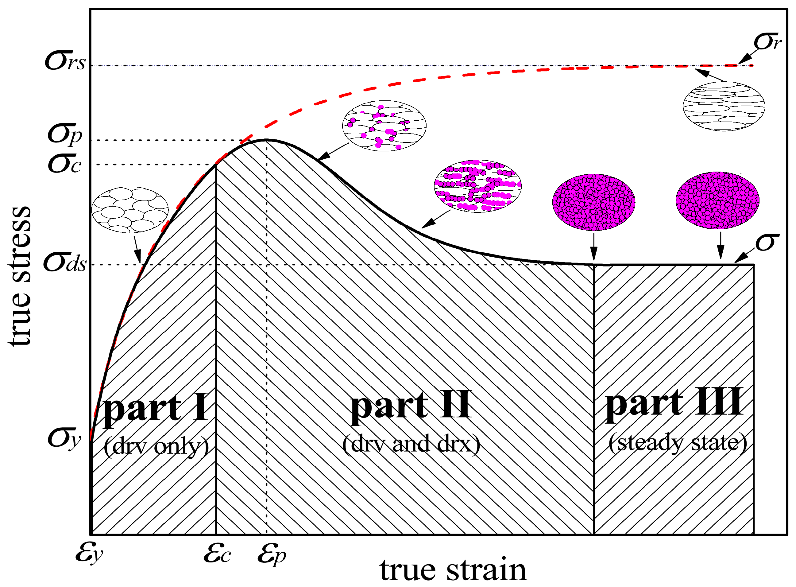
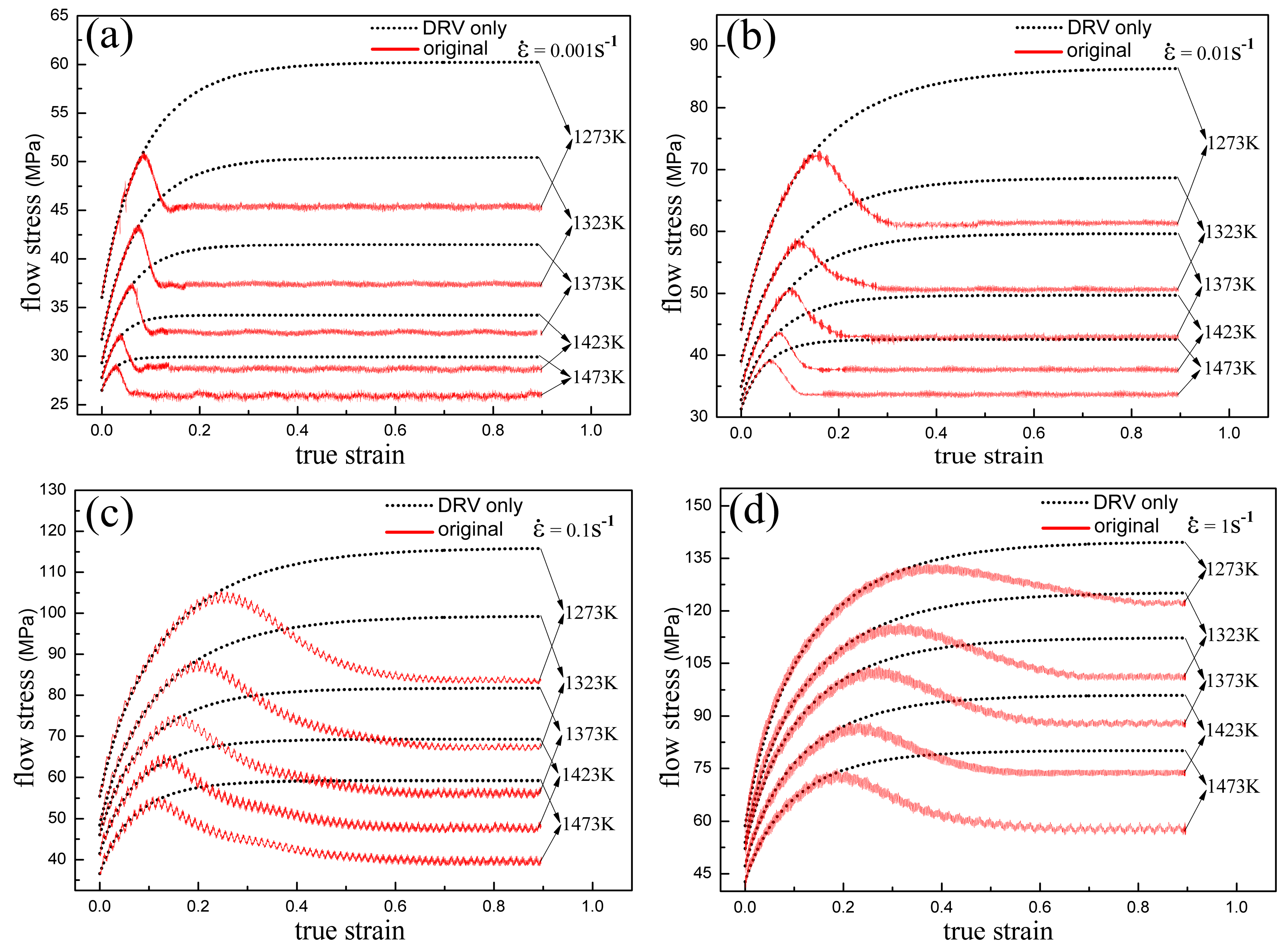
At the beginning of the hot deformation process, strain hardening initiates, which refers to the storage and annihilation (rearrangement) of dislocations [20]. Here the annihilation process is a dynamic recovery. The DRX process initiates when the dislocation density reaches an sufficient level to permit the nucleation of new grains. The new grains produce a softening and then decrease the work-hardening rate until eventually there is a clear stress peak. As volume fraction of new grains increases, more and more softening happens, and the flow stress decreases. After all the original microstructures transform into new grains, the strain hardening and strain softening reach a dynamic equilibrium, and then a steady state of flow stress appears [21,22]. According to the evolvement of the microstructure, the true stress-strain curve () is divided into three different parts: part I, part II and part III, and the schematic curve is shown in Figure 1. Here, part I is supposed to be the strain-hardening process before the DRX initiation. Micro-bands (MBs) usually appear in the austenite structure at this stage, which are formed by multiple cross-slips of dislocations or dislocation wall splitting [23,24]. Part II is the initiation of the DRX process, where the original microstructure transforms into new grains. The DRX process is supposed to be discontinuous in the austenite structure because of its low stacking fault energy, which inhibits DRV. The DRX grains in the austenite tend to nucleate through strain-induced boundary migration, e.g., the bulging of original grain boundaries, often accompanied by twinning [23,24]. Part III is supposed to be a steady state. As shown in the figure, DRX initiates at the critical strain and critical stress where part I changes to part II, peak strain and peak stress are supposed to be the point where falls to zero in part II, and is the steady stress which can also be determined from these points where is equal to zero in part III. The typical true stress-strain curves relating to DRX are presented in Figure 2a,b, and the grains corresponding to the steady state are isometric crystal, which is the typical microstructure of completed DRX.
Shown in Figure 1, the dashed curve () is supposed to be the one that resulted only from the restoration process of DRV, i.e., in the absence of DRX. It represents the assumed strain-hardening behavior of part I and the un-recrystallized regions in part II. Although it cannot be directly obtained from experiments related to DRX, this curve can be derived from the strain-hardening behavior of part I. In the dashed curve, the saturation state is attained when the dislocation annihilation has increased sufficiently to balance the dislocation storage, and then the stress () reaches a steady value. As shown in Figure 2c,d, the typical true stress-strain curves only relating to DRV are presented with low deformation temperatures, and the grains corresponding to the saturation state of these curves are elongated along the deformation direction, which is the typical microstructure with only the DRV process.
5. Constitutive Relationship in Hot Deformation
5.1. Constitutive Relationship of Part I
5.1.1. Constitutive Models Only Relating to DRV Process
When deformed in part I, the strain-hardening process is controlled by the competition of the storage and annihilation of dislocations. These two processes are supposed to superimpose in an opposite manner. In the KM model, the relation between the dislocation density and plastic strain is expressed as follows [10]:
where is an athermal constant associated with the storage process, is associated with the annihilation (DRV) process, and . Though the integration of Equation (1), the following equation can be obtained:
Because was defined as zero, can be derived as: . Then, Equation (2) can be expressed as follows:
As shown in the dashed curve of Figure 1, when in the saturation process. Therefore, according to Equation, (1), . Then, Equations (1) and (3) can be expressed as follows:
The relation between and the dislocation density is expressed as follows by [10]:
Therefore, , and in Equations (4) and (5) can be replaced by , , and , respectively. In this way, Equations (4) and (5) can be rewritten as follows:
As shown in Equation (8), this constitutive model presents the mathematic expression of the dashed line shown in Figure 1, and describes the constitutive relationships of part I and the un-recrystallized regions in part II.
5.1.2. Determination of Constant
According to Equation (7), presents a linear relation with . Meanwhile, through the linear regression of vs. , is obtained as the slope and can be calculated from the intercept. The relation between and of Armco-type pure iron is presented in Figure 3. As shown in the figure, the fitting linear curves before the DRX critical points are employed to determine the values of and for different temperatures and strain rates, and these calculated values are shown in the Supplementary Materials of Table S2. Based on the calculated values of , and the fitted values of , the flow stress curves only relating to the DRV process for Armco-type pure iron are calculated out through Equation (8) and presented in Figure 4. As discussed above, these flow stress curves stand for the work-hardening behavior of part I and the un-recrystallized regions in part II. As shown in Figure 4, these calculated curves fit well with the original true stress-strain curves in part I. Therefore, the flow behavior of part I with only the DRV process can be well described through Equation (8).
As presented in Equation (1), is the function of and . In order to completely describe the flow behavior of DRV, it is crucial to determine the equation of . According to Zener et al., and usually show combined effects on hot deformation in the form of the parameter [4]. Whether and show combined effects (e.g., in the form of the parameter) or individual effects on should be discussed. Therefore, the vs. curve shown in Figure 5 is employed to determine the relationship between the parameter and . Through polynomial fitting, the relation between the parameter and can be expressed as follows:
As shown in Equation (9), and present the combined effects on in the form of the parameter.
5.2. Constitutive Relationship of Part II
5.2.1. Avrami Kinetic Equation for DRX
The Avrami kinetic equation first proposed by Avrami has been widely used to describe the static recrystallization (SRX) process [25,26]. Although originally intended to quantify the progress of the recrystallized volume fraction, it has also been employed to describe the fractional softening later in the SRX process. The Avrami kinetic equation for SRX is usually expressed as follows:
Through some appropriate modifications, Equation (10) was used to describe the case of DRX by Jonas et al., Kim et al. and Quan et al. [27,28,29]. However, among these former modifications, the modified equations are not as accurate as is expected, or their expressions are very complicated. For example, Jonas et al. modified the Avrami equation as: , where is given by the expression of [27]. The expression is very complicated; therefore, it is very hard to determine the constants; additionally, its reliability also has not been clearly discussed. Kim et al. simplified the Avrami equation as: , where is the strain corresponding to the maximum softening rate [28]. The simplification promotes the application of Avrami kinetics to DRX, however, the accuracy is limited due to the neglect of the Avrami constant . In this paper, the original Avrami equation of Equation (10) is chosen to describe the volume fraction of recrystallized microstructures during the DRX process. Hot deformation usually refers to different temperatures and strain rates. Therefore, and are supposed to be the functions of and when using Equation (10) for the DRX process. DRX initiates at the critical strain, so for DRX can be replaced by: . According to these modifications, Equation (10) can be used to describe the DRX process, and the modified equation is expressed as follows:
where and .
5.2.2. Determination of Critical Strain
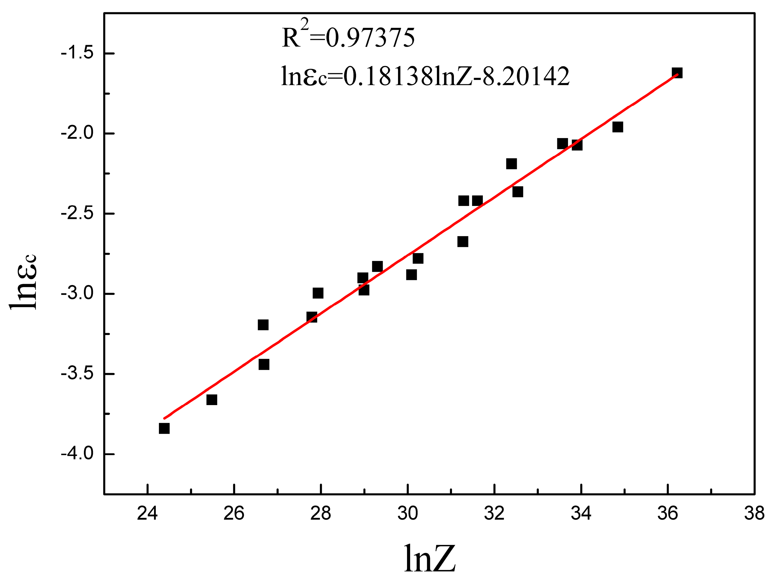
The DRX process initiates at the critical strain where part I changes to part II. Poliak et al. proposed that the critical state for the onset of DRX corresponds to an inflection point in the vs. curve [30]. Here is the work-hardening rate and expressed as: . According to mathematics, the inflection point corresponds to the peak point of the vs. curve. Therefore, in order to determine the critical state for Armco-type pure iron at different temperatures and strain rates, vs curves are calculated out and presented in Figure 6. As shown in the figure, is very close to , and the values are determined from the peak points of each curve. After determining , the corresponding can be obtained from the original true stress-strain curves, the values of which are shown in the Supplementary Materials of Table S2. Figure 7 presents the relationship between and the parameter. As shown in this figure, and present a linear relation. Through linear fitting, is expressed in the function of the parameter as follows:
As shown in Equation (12), and also present combined effects on in the form of the parameter.
5.2.3. Description of Fractional Softening
When deformed in part II, the DRX process initiates, and the restoration process is mainly a combination of DRX and DRV. The microstructures are divided into two regions in the part: the recrystallized regions and un-recrystallized regions. As presented in Equation (5), the dislocation density of un-recrystallized regions depends on the strain. Here, all the recrystallized regions in part II and part III are supposed to own same dislocation density . Then, the average dislocation density can be expressed as follows:
Combined with Equation (6), Equation (13) can be rewritten as follows:
Through the deduction of Equation (14), the fractional softening model in hot deformation can be expressed as follows:
The expression of Equation (15) is different from previous models. For example, as employed by Jonas et al., Serajzadeh et al. and Yang et al., fractional softening is expressed as: , and , respectively [27,31,32]. In these former expressions, the strain effect on the hardening process of un-recrystallized regions is neglected or not accurately considered, which reduces the reliability of these expressions. Equation (15) is constructed by taking into account the strain effect on the hardening process; meanwhile, the relation (shown in Equation (8)) between and is used to describe the strain-hardening process. Taking Equation (8) into Equation (15), the fractional softening model is expressed as follows:
Equation (16) is employed to describe fractional softening in this paper for a more accurate expression.
5.2.4. Determination of Avrami Constant and Time Exponent
As discussed above, through some proper modifications presented in Equation (11), the Avrami equation can be used to describe the DRX process. When using the modified Avrami equation for the DRX process, the expressions of and must be determined. Taking the natural logarithm twice on both sides of Equation (11), the following can be obtained:
As shown in Equation (17), and present a linear relationship where and serve as the slope and intercept, respectively. As shown in Figure 8, vs. curves are employed to determine the values of and at different temperatures and strain rates for Armco-type pure iron. Here, the recrystallized volume fraction in these curves is calculated via Equation (16). The values of and , obtained from the linear fitting, are presented in the Supplementary Materials of Table S2. As discussed above, and are supposed to be the function of and . Whether and show combined effects (e.g., in the form of the parameter) or individual effects on and also needs to be discussed.
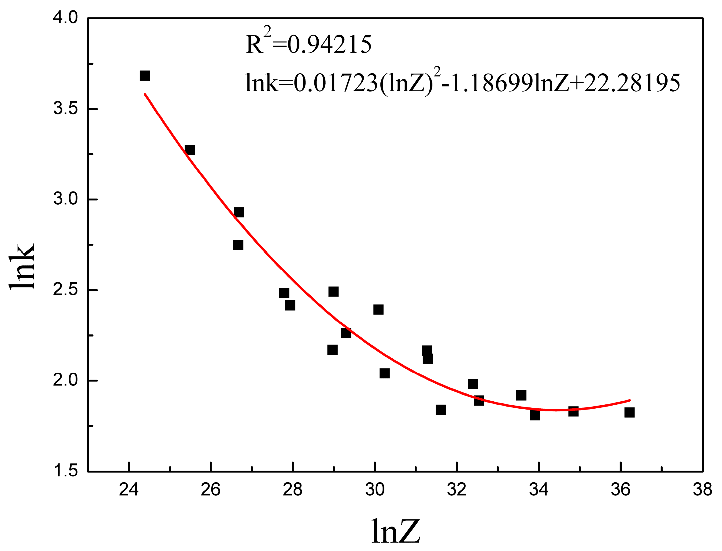
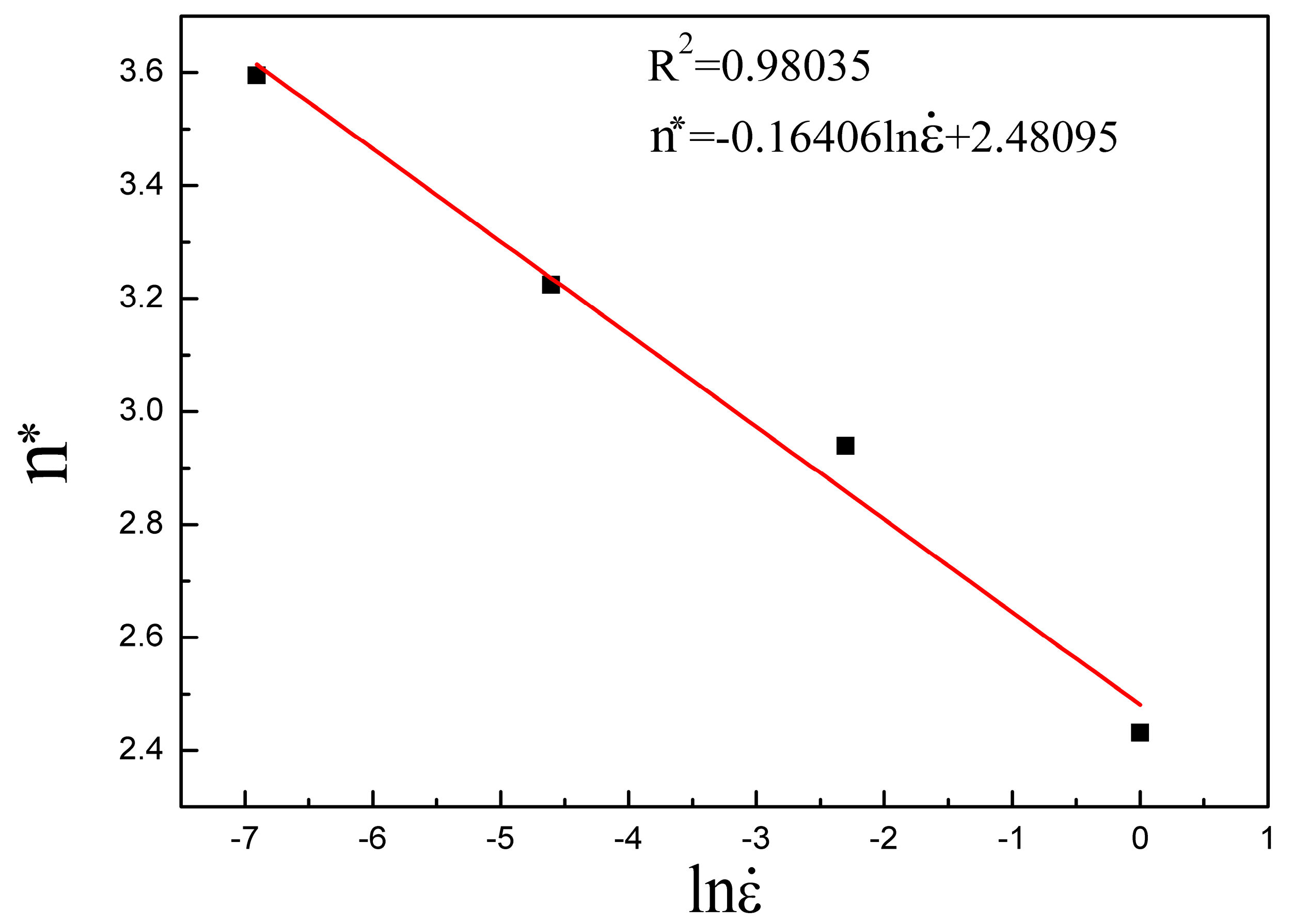
As shown in Figure 8, the values of the slope are nearly the same when in the same strain rates; meanwhile, the temperatures show no obvious effects. Here, the average values of for strain rates of 0.001 s−1, 0.01 s−1, 0.1 s−1 and 1 s−1 are 3.595144, 3.224808, 2.939272 and 2.43113, respectively. The relation between the average values and shown in Figure 9 is employed to determine the expression: . Through a linear fitting, is obtained as follows:
The relation between and shown in Figure 10 is employed to determine the expression: . As shown in the figure, and present a linear relationship when in the same strain rates. The slopes of these linear fitting curves are supposed to be same, and the average value is −0.3484. However, the intercepts are different, and the intercepts for strain rates of 0.001 s−1, 0.01 s−1, 0.1 s−1 and 1 s−1 are −3.89581, 2.99362, 9.56383 and 14.89145, respectively. Therefore, except for the combined effects of and on in the form of the parameter, also shows an individual effect, and can be expressed as follows:
where is the function representing the individual effect of the strain rate. The relation between the intercepts and strain rate inserted in Figure 10 is employed to determine the expression of . Through a linear fitting, is obtained as follows:
Taking Equation (20) into Equation (19), can be expressed as follows:
5.2.5. Constitutive Models Relating to the DRX and DRV Processes
Combined of Equations (11), (12), (18) and (21), the Avrami kinetic equation for Armco-type pure iron is expressed as follows:
The DRX process of Armco-type pure iron can be well described through Equation (22), which presents the influences of strain, strain rate and temperature on the DRX process. The S-curves of Armco-type pure iron are calculated out by Equation (22) and presented in Figure 11. As shown in the figure, when in same strain, the volume fraction of DRX increases with an increasing temperature and decreasing strain rate. Meanwhile, the critical strain of DRX increases with a decreasing temperature and increasing strain rate.
The constitutive relationship for alloys in hot deformation refers to the DRV process (un-recrystallized regions) and DRX process. The relation between these two processes can be described through Equation (14). Meanwhile, the DRV process can be described by Equation (8). Taking Equation (8) into Equation (14), the constitutive model for alloys in hot deformation can be expressed as follows:
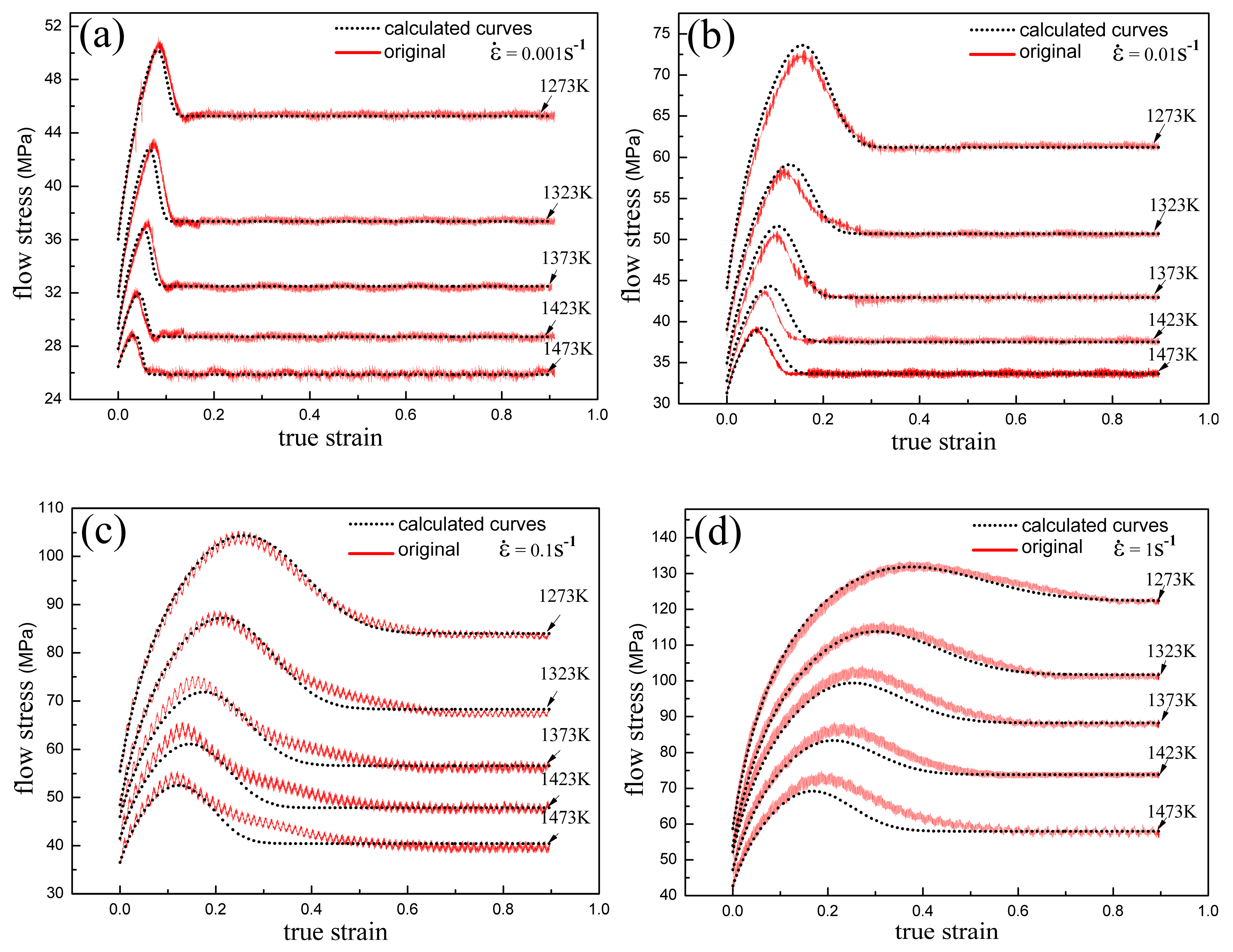
For Armco-type pure iron, and are expressed by Equations (9) and (22), respectively. Through Equation (23) and the values of , and provided in the Supplementary Materials of Table S2, the true stress-strain curves of Armco-type pure iron are calculated out and presented in Figure 12. As shown in the figure, these calculated curves fit well with the original true stress-strain curves in whole part, which means the flow behavior of alloys in hot deformation can be well described through Equation (23). However, the initial values of , and used in Equation (23) have all been obtained from polynomial fitting. For the completion of Equation (23), it is meaningful to determine the expressions of , and .
5.3. Constitutive Relationship of Part III
5.3.1. Constitutive Model of Part III
When deformed in part III, the flow stress reaches a steady state , and all the original microstructures are completely recrystallized. Beladi et al. and Graetz et al. proposed that the recrystallized grain size is decreased as long as the strain rate increases and the temperature decreases, which is independent of the initial grain size and strain [21,22]. As discussed above, the precision of Arrhenius-type equations is reduced due to the neglect of the strain effects. However, the strain effects need no consideration when in a steady state where the flow stress is independent of the strain; therefore, using Arrhenius-type equations to describe the flow behavior of the steady state is appropriate. According to different hot deformation conditions, Arrhenius-type equations based of the Z parameter can be expressed as follows:
The stress multiplier is defined as: . As proposed by Mandal et al. and Lin et al., Equation (24) is preferred for a low strain level where < 0.8, while Equation (25) is preferred for a high strain level where > 1.2 [33,34]. The sine-hyperbolic equation of Equation (26), proposed by Sellars et al., is widely employed to describe the relationship between flow stress, strain rate and deformation temperature over a wide range of stresses [14]. Therefore, Equation (26) is used to describe the flow behavior of the steady state in this work. According to Equation (26), the constitutive model for part III can be expressed as follow:
5.3.2. Determination of Constants , and
Taking the natural logarithm of both sides of Equations (24), (25) and (26), the following forms can be obtained:
With respect to temperature, the partial differentiations of Equations (28), (29) and (30) yield the following:
With respect to the strain rate, the partial differentiation of Equation (30) yields the following:
The values of presented in the Supplementary Materials of Table S1, and the corresponding strain rates and temperatures, are used to determine the values of these constants. As shown in Figure 13, using the linear regression of these data, the values of , and obtained as the average slopes of -, - and -, are 7.37182, 0.13345 and 5.50432, respectively. Meanwhile, the value of obtained as the average value of is 0.01777, and the value of calculated based on the average slopes of - is 383094 J mol−1. The activation energy of Armco-type pure iron is lower than that of other steels, and this is mainly caused by the high Fe atom purity. Alloy elements in other steels usually decrease the mobility of Fe atoms and thus increase the value of . According to the calculated value of , the Z parameter for Armco-type pure iron can be expressed as follows:
According to Equation (30) the value of can be gained as the intercept of the plot. Through the linear regression shown in Figure 14, the value of is 29.6307, and is 7.38668 × 10¹². Taking the values of , and into Equation (27), the constitutive model for Armco-type pure iron in part III can be expressed as follows:
5.4. Integrated Constitutive Relationship for Hole Part
5.4.1. Determination of Yield Stress and Saturation Stress
Figure 15 presents the relations between , and the parameter. Shown in the figure, and show combined effects on and in the form of the parameter. Meanwhile, and present linear relations with . Through linear fitting, the expressions of and for Armco-type pure iron can be expressed as follows:
5.4.2. Avrami Kinetic-Based Constitutive Model of Whole Part
Integrating expressions of Equations (11) and (23), the Avrami kinetic-based constitutive model for alloys considering the effects of DRV and DRX can be expressed as follows:
As discussed above for Armco-type pure iron, , , , , , and are expressed as follows:
Using Equations (39) and (40), the flow behavior of Armco-type pure iron is well described, and the flow stress curves calculated out through these two equations are presented in Figure 16. As shown in the figure, the strain effects are considered, especially for these parts before the steady state; meanwhile, the DRV and DRX characters referring to strain hardening, and the stress peak are well presented in these curves.
6. Conclusions
The work presents a full mathematical description of the stress-strain compression curves in a wide range of strain rates and deformation temperatures. The constructed models are based on the dislocation structure evolution equation (in the case of DRV) and Avrami kinetic-based model (in the case of DRX). Based on this study, the following can be concluded:
- (1)
- Based on the KM model, the strain-hardening process relating only to DRV can be described by the equation: . is determined by the part of the true stress-strain curve before the initiation of DRX. As for Armco-type pure iron, and show combined effects on , and in the form of the Z parameter with expressions as: , and , respectively.
- (2)
- Considering the strain-hardening process, the model used to describe the fractional softening for alloys under DRX is modified as: . The volume fraction of DRX increases as long as the temperature increases and the strain rate decreases. The critical points for the onset of DRX are determined as the inflection point in the vs. curve. As for Armco-type pure iron, the relation between and the Z parameter is expressed as: .
- (3)
- The Avrami kinetic equation is used to describe the kinetic of DRX with the modified expression as: , where and . As for Armco-type pure iron, including an individual effect, the strain rate also presents a combined effect with on in the form of the Z parameter, and the relation is expressed as: . is only the function of with the expression: .
- (4)
- Arrhenius-type equations are suitable for describing the flow behavior of the steady state. Regressing from the equations, the DRX activation energy for Armco-type pure iron is 383094 J mol−1, and the expressions for the parameter and are determined as Equations (35) and (36), respectively.
- (5)
- Based on strain hardening, fractional softening models and the modified Avrami kinetic equation, the constitutive model for alloys considering the effects of DRV and DRX is constructed as Equation (39). The constitutive model can be well used to describe the flow behavior of Armco-type pure iron. The DRV and DRX characters are clearly presented in these curves determined by this model.
Supplementary Materials
The following are available online at https://www.mdpi.com/2075-4701/9/3/365/s1, Table S1. Fitted values of Armco-type pure iron; Table S2. Calculated values of Armco-type pure iron.
Author Contributions
Conceptualization, Q.F. and Y.Z.; methodology, Y.Z.; software, Y.Z.; validation, Y.Z.; formal analysis, Y.Z.; investigation, Y.Z.; resources, X.Z.; data curation, Y.Z.; writing—original draft preparation, Y.Z.; writing—review and editing, Y.Z.; visualization, Y.Z.; supervision, Z.Z. project administration, Z.X.; funding acquisition, Z.Q.
Funding
This research received no external funding.
Acknowledgments
Thanks for the support from my love, my family and group colleagues.
Conflicts of Interest
The authors declare no conflict of interest. The funders had no role in the design of the study; in the collection, analyses, or interpretation of data; in the writing of the manuscript, or in the decision to publish the results.
Nomenclature
| strain rate (s−1) | |
| temperature (K) | |
| activation energy (J mol−1) | |
| universal gas constant (8.31 J mol−1K−1) | |
| Zener–Hollomon parameter | |
| strain | |
| yield strain | |
| strain at maximum softening rate | |
| , | critical strain and critical stress (MPa) |
| , | peak strain and peak stress (MPa) |
| , | flow stress (MPa) and steady value of it |
| , | recovery stress (MPa) and saturation value of it |
| average dislocation density corresponding to whole deforming process | |
| dislocation density corresponding to only DRV process | |
| dislocation density at yield point | |
| dislocation density at the steady state of flow stress | |
| dislocation density at the saturation state of recovery stress | |
| shear modulus | |
| burgers vector | |
| recrystallized volume fraction | |
| Avrami constant | |
| time (s) | |
| characteristic time | |
| time exponent | |
| grain size | |
| , , , , , , , , , , , , | constants |
References
- McQueen, H.J.; Ryan, N.D. Constitutive analysis in hot working. Mater. Sci. Eng. A 2002, 322, 43–63. [Google Scholar] [CrossRef]
- He, Z.B.; Wang, Z.B.; Lin, Y.L.; Fan, X.B. Hot Deformation behavior of a 2024 aluminum alloy sheet and its modeling by Fields-Backofen model considering strain rate evolution. Metals 2019, 9, 243. [Google Scholar] [CrossRef]
- Salinas, A.; Celentano, D.; Carvajal, L.; Artigas, A.; Monsalve, A. Microstructure-Based Constitutive Modelling of Low-Alloy Multiphase TRIP Steels. Metals 2019, 9, 250. [Google Scholar] [CrossRef]
- Zener, C.; Hollomon, J.H. Effect of strain rate upon plastic flow of steel. J. Appl. Phys. 1944, 15, 22–32. [Google Scholar] [CrossRef]
- Johnson, G.R.; Cook, W.H. Fracture characteristics of three metals subjected to various strains, strain rates, temperatures and pressures. Eng. Fract. Mech. 1985, 21, 31–48. [Google Scholar] [CrossRef]
- Ulacia, I.; Salisbury, C.P.; Hurtado, I.; Worswick, M.J. Tensile characterization and constitutive modeling of AZ31B magnesium alloy sheet over wide range of strain rates and temperatures. J. Mater. Process. Technol. 2011, 211, 830–839. [Google Scholar] [CrossRef]
- Bhattacharya, R.; Lanc, Y.J.; Wynne, B.P.; Davis, B.; Rainforth, W.M. Constitutive equations of flow stress of magnesium AZ31 under dynamically recrystallizing conditions. J. Mater.Process. Technol. 2014, 214, 1408–1417. [Google Scholar] [CrossRef]
- Gambirasio, L.; Rizzi, E. On the calibration strategies of the Johnson–Cook strength model: Discussion and applications to experimental data. Mater. Sci. Eng. A 2014, 610, 370–413. [Google Scholar] [CrossRef]
- Zerilli, F.J.; Armstrong, R.W. Dislocation-mechanics-based constitutive relations for material dynamics calculations. J. Appl. Phys. 1987, 61, 1816–1825. [Google Scholar] [CrossRef] [Green Version]
- Estrin, Y.; Mecking, H. A unified phenomenological description of work hardening and creep based on one-parameter models. Acta Metall. 1984, 32, 57–70. [Google Scholar] [CrossRef]
- Choudhary, B.K.; Christopher, J. Comparative tensile flow and work-hardening behavior of 9 Pct chromium ferritic-martensitic steels in the framework of the Estrin-Mecking internal-variable approach. Metall. Mater. Trans. A 2016, 47, 2642–2655. [Google Scholar] [CrossRef]
- Haghdadi, N.; Martin, D.; Hodgson, P. Physically-based constitutive modeling of hot deformation behavior in a LDX 2101 duplex stainless steel. Mater. Des. 2016, 106, 420–427. [Google Scholar] [CrossRef]
- Chalimba, S.A.; Mostert, R.; Stumpf, W.; Siyasiya, C.; Banks, K. Modeling of work hardening during hot rolling of vanadium and niobium microalloyed steels in the low temperature austenite region. J. Mater. Eng. Perform. 2017, 26, 5217–5227. [Google Scholar] [CrossRef]
- Sellars, C.M.; Tegart, W.M. On the mechanism of hot deformation. Acta Metall. 1966, 14, 1136–1138. [Google Scholar] [CrossRef]
- Li, J.D.; Liu, J.S. Strain Compensation Constitutive Model and Parameter Optimization for Nb-Contained 316LN. Metals 2019, 9, 212. [Google Scholar] [CrossRef]
- Tabei, A.; Abed, F.H.; Voyiadjis, G.Z.; Garmestani, H. Constitutive modeling of Ti-6Al-4V at a wide range of temperatures and strain rates. Eur. J. Mech.-A/Solids 2017, 63, 128–135. [Google Scholar] [CrossRef]
- Zhang, C.S.; Ding, J.; Dong, Y.Y.; Zhao, G.Q.; Gao, A.J.; Wang, L.J. Identification of friction coefficients and strain-compensated Arrhenius-type constitutive model by a two-stage inverse analysis technique. Int. J. Mech. Sci. 2015, 98, 195–204. [Google Scholar] [CrossRef]
- Kugler, G.; Turk, R. Modeling the dynamic recrystallization under multi-stage hot deformation. Acta Mater. 2004, 52, 4659–4668. [Google Scholar] [CrossRef]
- Martin, E.; Jonas, J.J. Evolution of microstructure and microtexture during the hot deformation of Mg–3% Al. Acta Mater. 2010, 58, 4253–4266. [Google Scholar] [CrossRef]
- Tian, B.; Lind, C.; Schafler, E.; Paris, O. Evolution of microstructures during dynamic recrystallization and dynamic recovery in hot deformed Nimonic 80a. Mater. Sci. Eng. A 2004, 367, 198–204. [Google Scholar] [CrossRef]
- Beladi, H.; Cizek, P.; Hodgson, P.D. On the characteristics of substructure development through dynamic recrystallization. Acta Mater. 2010, 58, 3531–3541. [Google Scholar] [CrossRef]
- Graetz, K.; Miessen, C.; Gottstein, G. Analysis of steady-state dynamic recrystallization. Acta Mater. 2014, 67, 58–66. [Google Scholar] [CrossRef]
- Haghdadi, N.; Cizek, P.; Beladi, H.; Hodgson, P.D. The austenite microstructure evolution in a duplex stainless steel subjected to hot deformation. Philos. Mag. 2017, 97, 1209–1237. [Google Scholar] [CrossRef]
- Babu, K.A.; Mandal, S.; Athreya, C.N.; Shakthipriya, B.; Sarma, V.S. Hot deformation characteristics and processing map of a phosphorous modified super austenitic stainless steel. Mater. Des. 2017, 115, 262–275. [Google Scholar] [CrossRef]
- Avrami, M. Kinetics of phase change. I. General theory. J. Chem. Phys. 1939, 7, 1103–1112. [Google Scholar] [CrossRef]
- Avrami, M. Kinetics of phase change. II. Transformation-time relations for random distribution of nuclei. J. Chem. Phys. 1940, 8, 212–224. [Google Scholar] [CrossRef]
- Jonas, J.J.; Quelennec, X.; Jiang, L.; Martin, E. The Avrami kinetics of dynamic recrystallization. Acta Mater. 2009, 57, 2748–2756. [Google Scholar] [CrossRef]
- Kim, S.I.; Yoo, Y.C. Dynamic recrystallization behavior of AISI 304 stainless steel. Mater. Sci. Eng. A 2001, 311, 108–113. [Google Scholar] [CrossRef]
- Quan, G.Z.; Wu, D.S.; Luo, G.C.; Xia, Y.F.; Zhou, J.; Liu, Q.; Gao, L. Dynamic recrystallization kinetics in α phase of as-cast Ti–6Al–2Zr–1Mo–1V alloy during compression at different temperatures and strain rates. Mater. Sci. Eng. A 2014, 589, 23–33. [Google Scholar] [CrossRef]
- Poliak, E.I.; Jonas, J.J. A one-parameter approach to determining the critical conditions for the initiation of dynamic recrystallization. Acta Mater. 1996, 44, 127–136. [Google Scholar] [CrossRef]
- Serajzadeh, S.; Taheri, A.K. An investigation on the effect of carbon and silicon on flow behavior of steel. Mater. Des. 2002, 23, 271–276. [Google Scholar] [CrossRef]
- Yang, Z.; Guo, Y.C.; Li, J.P.; He, F.; Xia, F.; Liang, M.X. Plastic deformation and dynamic recrystallization behaviors of Mg–5Gd–4Y–0.5Zn–0.5Zr alloy. Mater. Sci. Eng. A 2008, 485, 487–491. [Google Scholar] [CrossRef]
- Mandal, S.; Rakesh, V.; Sivaprasad, P.V.; Venugopal, S.; Kasiviswanathan, K.V. Constitutive equations to predict high temperature flow stress in a Ti-modified austenitic stainless steel. Mater. Sci. Eng. A 2009, 500, 114–121. [Google Scholar] [CrossRef]
- Lin, Y.C.; Xia, Y.C.; Chen, X.M.; Chen, M.S. Constitutive descriptions for hot compressed 2124-T851 aluminum alloy over a wide range of temperature and strain rate. Comput. Mater. Sci. 2010, 50, 227–233. [Google Scholar] [CrossRef]
Figure 1.
Schematic illustration of the microstructure evolvement and the division of the true stress-strain curve in the hot deformation process. According to the difference of the microstructure evolvement, the true stress-strain curve () is divided into three parts (part I, part II and part III). Part I undergoes the dynamic recovery (DRV) process. Part II is the initiation of the dynamic recrystallization (DRX) process while these un-recrystallized regions still undergo the DRV process. Part III is the steady state; all the original microstructure has been recrystallized and reaches a dynamic equilibrium in this part. The dashed curve ( ) represents the work-hardening behavior of part I and the un-recrystallized regions in part II.

Figure 2.
Microstructure of Armco-type pure iron deformed at different conditions: (a) = 1s−1, = 1423K; (b) = 1s−1, = 1373K; (c) = 1s−1, = 1023K; and (d) = 1s−1, = 973K. (a,b) relate to the completed DRX process in the hot deformation, while (c,d) relate to the DRV process with the deformation temperature lower than that of the hot deformation. The inserted figures are the corresponding true stress- strain cures.
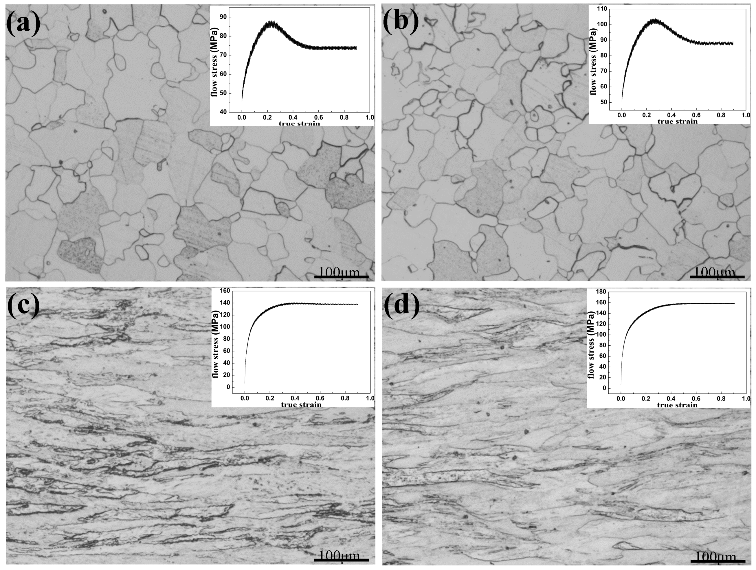
Figure 3.
vs. plots derived from the true stress-strain curves of Armco-type pure iron: (a) = 0.001 s−1; (b) = 0.01 s−1; (c) = 0.1 s−1; and (d) = 1 s−1. The part before the DRX critical point of each curve refers to the DRV process and is fitted by the linear curve of the dot line. These linear curves are employed to determine the values of and . The method to determine the DRX critical points will be discussed later.

Figure 4.
Original true stress-strain curves and calculated flow stress curves considering only the DRV process of Armco-type pure iron: (a) = 0.001 s−1; (b) = 0.01 s−1; (c) = 0.1 s−1; and (d) = 1 s−1. The red solid curves are the original true stress-strain curves while the dot lines are the curves calculated through Equation (8). The dot lines describe the work-hardening behavior of part I and the un-recrystallized regions in part II.

Figure 5.
The relationship between the Z parameter and . The curve is obtained from polynomial fitting in the order of two. Here, the parameter is in the form of which is calculated in following chapter.
Figure 5.
The relationship between the Z parameter and . The curve is obtained from polynomial fitting in the order of two. Here, the parameter is in the form of which is calculated in following chapter.

Figure 6.
vs. curves of Armco-type pure iron: (a) = 0.001 s−1; (b) = 0.01 s−1; (c) = 0.1 s−1; and (d) = 1 s−1. According to the Poliak method, the DRX critical point is supposed to be the peak point of each curve [30]. The dashed lines correspond to the peak stresses of each curve.
Figure 6.
vs. curves of Armco-type pure iron: (a) = 0.001 s−1; (b) = 0.01 s−1; (c) = 0.1 s−1; and (d) = 1 s−1. According to the Poliak method, the DRX critical point is supposed to be the peak point of each curve [30]. The dashed lines correspond to the peak stresses of each curve.

Figure 7.
The relationship between the Z parameter and . The linear curve is obtained from linear fitting. Here, the parameter is in the form of .
Figure 7.
The relationship between the Z parameter and . The linear curve is obtained from linear fitting. Here, the parameter is in the form of .

Figure 8.
vs. curves of Armco-type pure iron: (a) = 0.001 s−1; (b) = 0.01 s−1; (c) = 0.1 s−1; and (d) = 1 s−1. The values of are calculated out through Equation (16). The dot lines are the linear fitting results of each curve. After the linear fitting, and are obtained as the slope and intercept, respectively.

Figure 9.
The relationship between and . The linear curve is obtained from linear fitting.

Figure 10.
The relationship between the Z parameter and . These linear curves are obtained from the linear fitting of points with the same strain rates. Here, the parameter is in the form of . Insert: the relationship between and the intercepts of these linear fitting curves.
Figure 10.
The relationship between the Z parameter and . These linear curves are obtained from the linear fitting of points with the same strain rates. Here, the parameter is in the form of . Insert: the relationship between and the intercepts of these linear fitting curves.
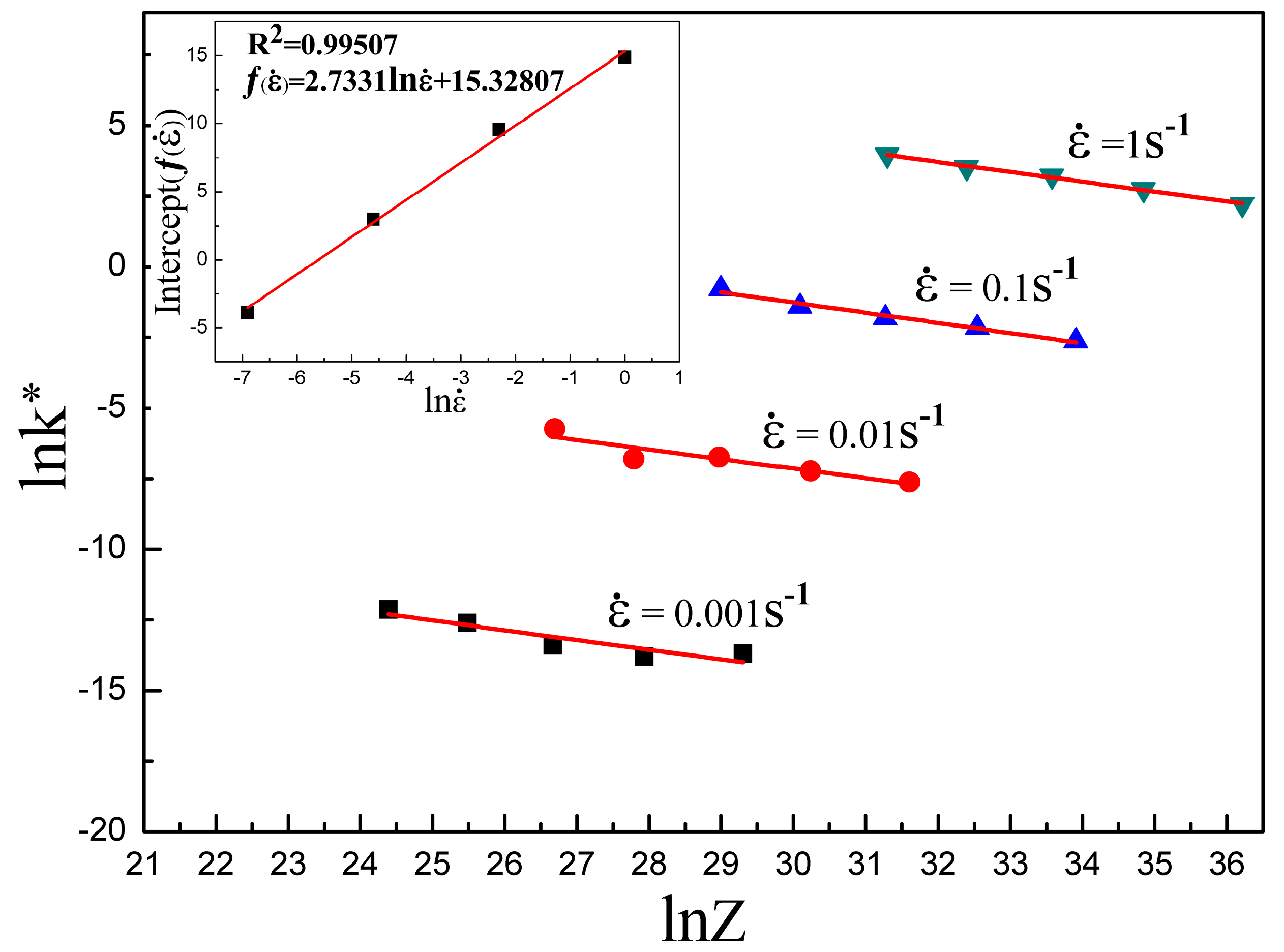
Figure 11.
S-curves of Armco-type pure iron calculated by Equation (22): (a) = 0.001 s−1; (b) = 0.01 s−1; (c) = 0.1 s−1; and (d) = 1 s−1.
Figure 11.
S-curves of Armco-type pure iron calculated by Equation (22): (a) = 0.001 s−1; (b) = 0.01 s−1; (c) = 0.1 s−1; and (d) = 1 s−1.

Figure 12.
Original true stress-strain curves and calculated flow stress curves considering eDRV and DRX processes of Armco-type pure iron: (a) = 0.001 s−1; (b) = 0.01 s−1; (c) = 0.1 s−1; and (d) = 1 s−1. The red solid curves are the original true stress-strain curves while the dot lines are the flow stress curves calculated through Equation (23).

Figure 13.
The relationships between , and : (a) and ; (b) and ; (c) and ; and (d) and . The linear curves are obtained from linear fitting.
Figure 13.
The relationships between , and : (a) and ; (b) and ; (c) and ; and (d) and . The linear curves are obtained from linear fitting.
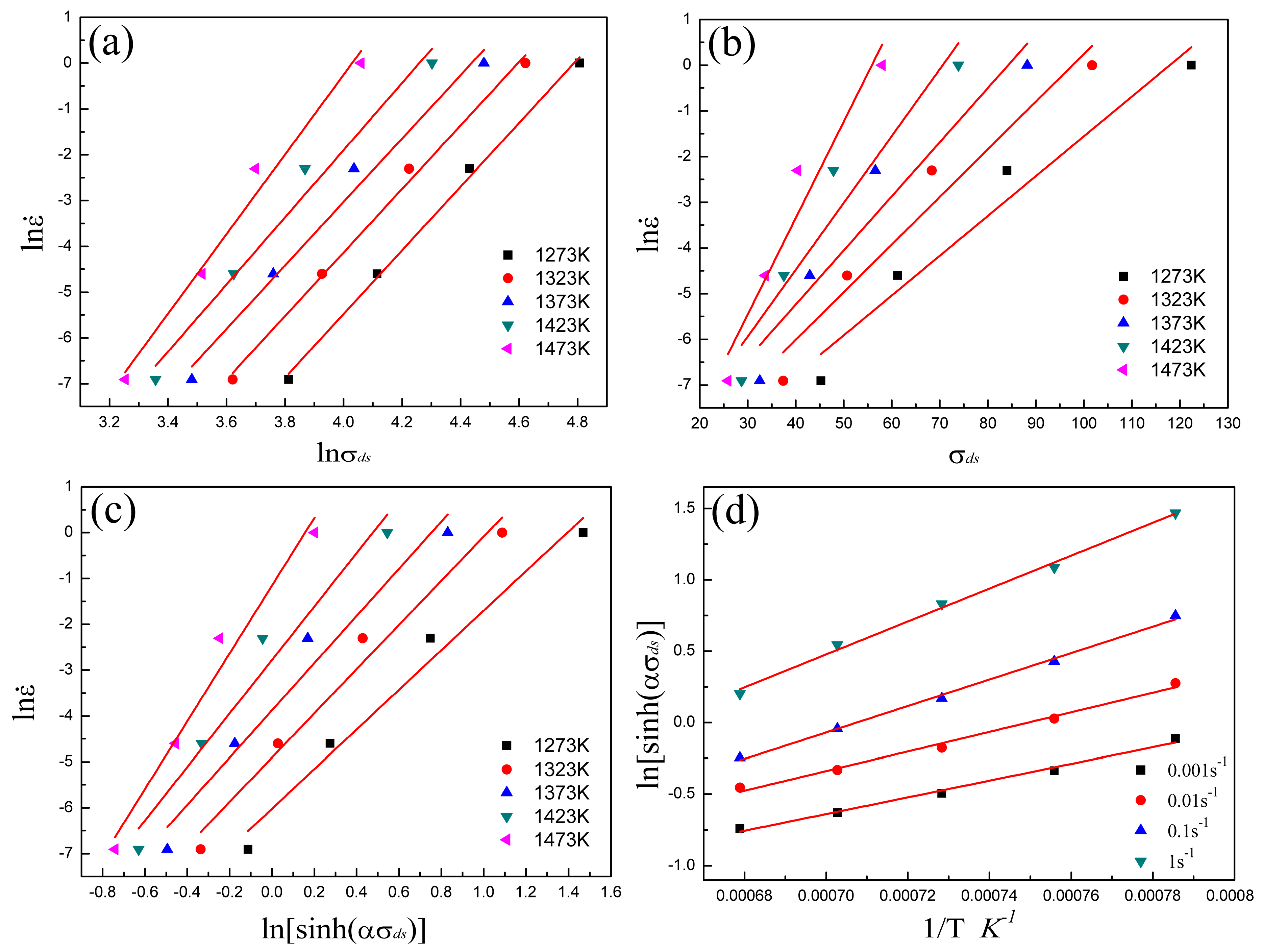
Figure 14.
Relationship between Z parameter and . The linear curve is got from linear fitting.
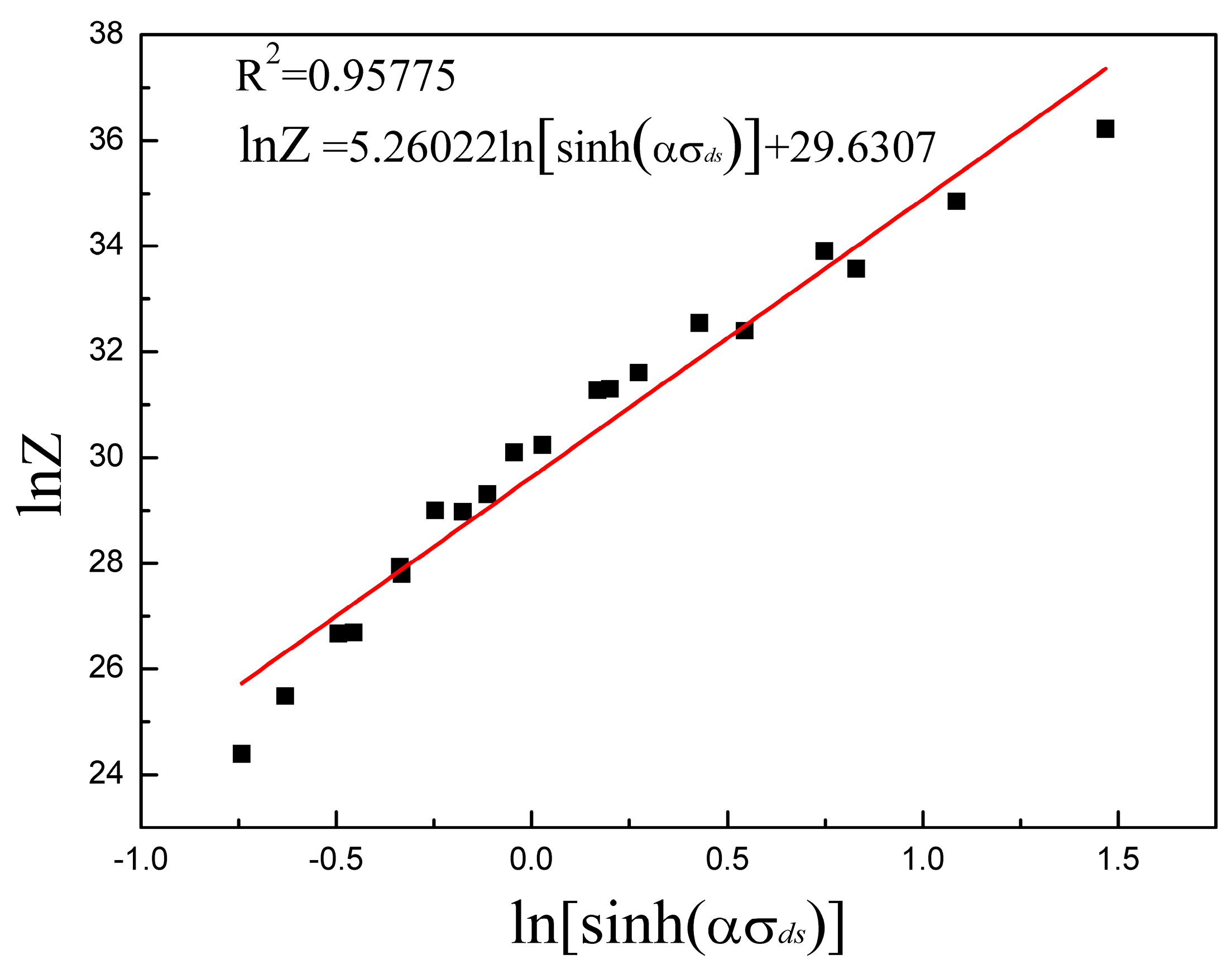
Figure 15.
The relationships between , and the parameter. The linear curves are obtained from linear fitting.
Figure 15.
The relationships between , and the parameter. The linear curves are obtained from linear fitting.

Figure 16.
Calculated flow stress curves using the Avrami kinetic-based constitutive model of Armco-type pure iron: (a) = 0.05 s−1; (b) = 0. 1 s−1; (c) = 0.5 s−1; and (d) = 1 s−1.
Figure 16.
Calculated flow stress curves using the Avrami kinetic-based constitutive model of Armco-type pure iron: (a) = 0.05 s−1; (b) = 0. 1 s−1; (c) = 0.5 s−1; and (d) = 1 s−1.


Table 1.
The chemical composition of Armco-type pure iron (at.%).
| C | Si | Mn | P | S |
|---|---|---|---|---|
| 0.0019 | 0.0294 | 0.1298 | 0.0056 | 0.0038 |
© 2019 by the authors. Licensee MDPI, Basel, Switzerland. This article is an open access article distributed under the terms and conditions of the Creative Commons Attribution (CC BY) license (http://creativecommons.org/licenses/by/4.0/).
Share and Cite
MDPI and ACS Style
Zhang, Y.; Fan, Q.; Zhang, X.; Zhou, Z.; Xia, Z.; Qian, Z. Avrami Kinetic-Based Constitutive Relationship for Armco-Type Pure Iron in Hot Deformation. Metals 2019, 9, 365. https://doi.org/10.3390/met9030365
AMA Style
Zhang Y, Fan Q, Zhang X, Zhou Z, Xia Z, Qian Z. Avrami Kinetic-Based Constitutive Relationship for Armco-Type Pure Iron in Hot Deformation. Metals. 2019; 9(3):365. https://doi.org/10.3390/met9030365
Chicago/Turabian StyleZhang, Yan, Qichao Fan, Xiaofeng Zhang, Zhaohui Zhou, Zhihui Xia, and Zhiqiang Qian. 2019. "Avrami Kinetic-Based Constitutive Relationship for Armco-Type Pure Iron in Hot Deformation" Metals 9, no. 3: 365. https://doi.org/10.3390/met9030365
Note that from the first issue of 2016, this journal uses article numbers instead of page numbers. See further details here.