Article

Atmospheric Corrosion Sensor Based on Strain Measurement with an Active Dummy Circuit Method in Experiment with Corrosion Products

1
Department of Risk Management and Environmental Sciences, Graduate School of Environmental and Information Sciences, Yokohama National University, Yokohama 240-8501, Japan
2
Department of Electrical Engineering, Faculty of Engineering, Lampung University, Bandar Lampung 35141, Indonesia
3
Division of Material Science and Engineering, Graduate School of Engineering, Yokohama National University, Yokohama 240-8501, Japan
4
Nippon Steel Research Institute, Tokyo 100-0005, Japan
5
RACE (Research into Artifacts, Center for Engineering), University of Tokyo, Japan
*
Author to whom correspondence should be addressed.
Metals 2019, 9(5), 579; https://doi.org/10.3390/met9050579
Submission received: 22 April 2019 / Revised: 9 May 2019 / Accepted: 16 May 2019 / Published: 18 May 2019
(This article belongs to the Special Issue Corrosion and Protection of Metals)

Abstract

:
This study analyzed an atmospheric corrosion sensor using strain measurements (ACSSM) with an active dummy method for corrosion product experiments. An initial compensation thermal strain experiment was performed with elapsed time. Further analyses used dry-wet environments with salt water spray to investigate the thickness reduction performance of the corrosion product on low-carbon steel samples. The ACSSM with an active dummy method accurately measured signals induced by the specimen thickness reduction, despite the noise in the signal. Moreover, the effects of corrosion products on the signal were discussed.

1. Introduction

Because corrosion damages materials in structures located outside, studies on atmospheric corrosion processes have received special attention from researchers. Morcillo et al [1] studied the nature of corrosion products, the mechanisms, and kinetics of the corrosion process, the morphology of steel rust, and long-term atmospheric corrosion monitoring. Song and Saraswathy [2] reported on methods and durability problems for monitoring corrosion in reinforced concrete structures. Wen et al [3] studied carbon steel corrosion products and their classification, effects on subsequent corrosion processes, and the dependence of the initiation, growth, and transformation processes in H2S environments on such products. Ahmad [4] investigated reinforcement corrosion in concrete structures including the mechanism of reinforcement corrosion, techniques for monitoring reinforcement corrosion, and methodologies to predict the remaining service lifetimes of structures.
In addition, many researchers have developed sensors to detect atmospheric corrosion using radio-frequency identification (RFID) sensors [5,6,7], passive wireless sensors [8], corrosion potential sensors [9], optic sensors, fibre Bragg gratings (FBGs) [10,11,12,13,14,15], atmospheric corrosion monitoring (ACM) methods [16,17], and atmospheric corrosion rate monitoring (ACRM) techniques [18].
Several techniques for atmospheric corrosion monitoring, such as weight and thickness loss measurement [19,20,21,22], electrochemical impedance spectroscopy (EIS) [23,24,25], microscopy and scanning electron microscopy (SEM) [26,27], and X-ray diffraction (XRD) [28,29] have been established as necessary.
A strain measurement method using strain gauges for in situ corrosion monitoring was proposed in our previous study [30,31]. However, precise monitoring was difficult because the strain measurement method was very sensitive to temperature drift. Thus, a highly accurate in situ method for monitoring atmospheric corrosion remains necessary. The strain-measurement circuit using the active dummy method for an atmospheric corrosion sensor based on strain measurement (ACSSM) with strain gauges accommodated such temperature drifts and showed good performance in the situ monitoring of specimen thinning under corrosion, as measured by galvanostatic electrolysis [32,33,34]. However, for actual applications, experiments with dry-wet method [35,36,37,38] to investigate the performance of the corrosion product/rust under strain behavior.
This study conducted experiments with the dry-wet method by applying a 5% NaCl solution to test pieces in order to investigate the performance of ACSSM via the active dummy method. Thickness changes, obtained from the weight loss of the specimens, were monitored simultaneously. Based on the experimental findings, the performance of the ACSSM and the effect of corrosion products on the signal were discussed.

2. Methods

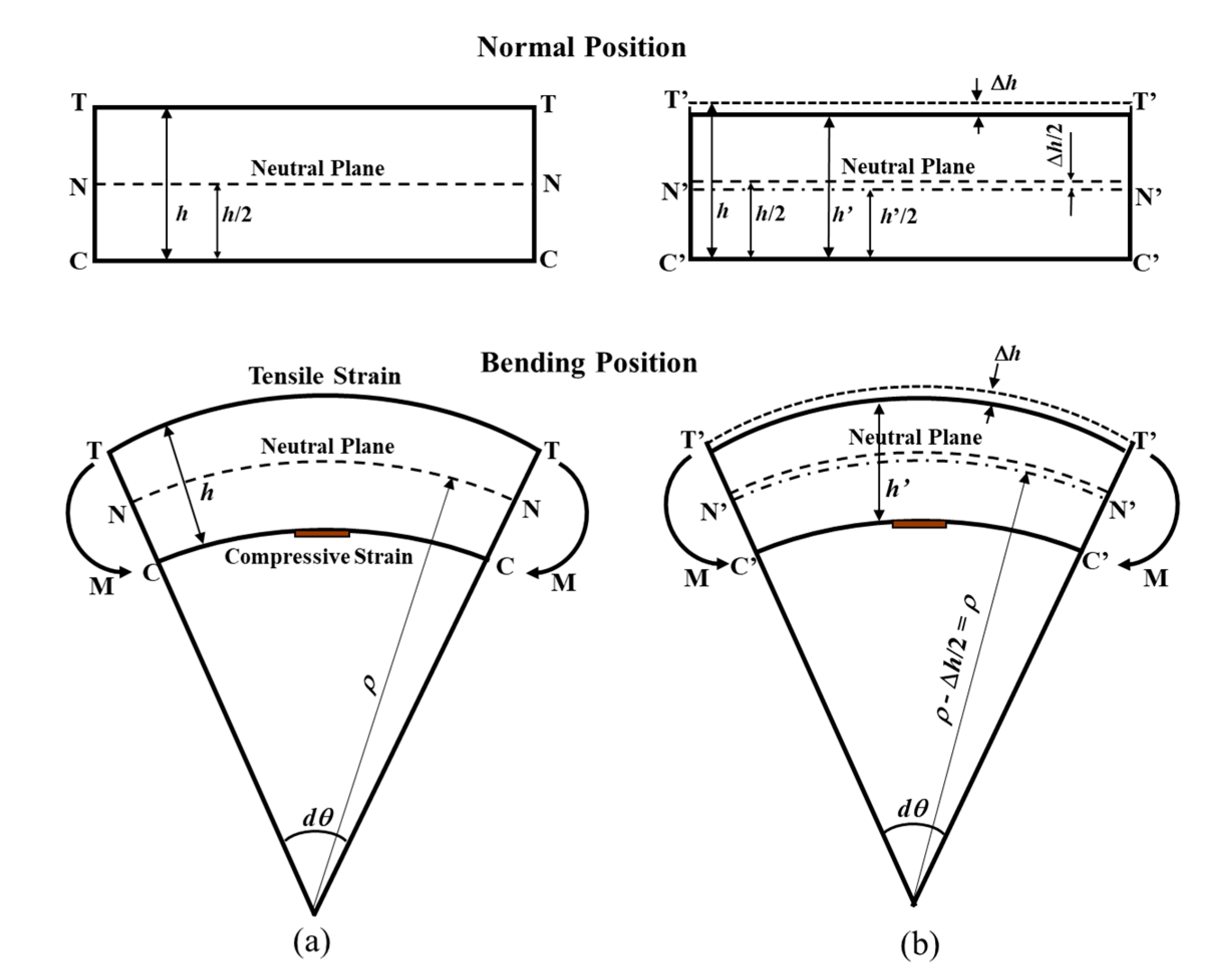
2.1. Concept of the ACSSM

According to [30,31], the strain on the compressive surface of a low-carbon (mild) steel test piece under a bending moment can be expressed by:
ε = −h/2ρ
where ε is the strain in the test piece (×10−6 ε), ρ is the radius of curvature of the test piece (mm), h is the test piece thickness (mm), and dθ is the center angle of curvature of the test piece. Figure 1 shows the mechanical principle for the ACSSM sensor in normal and bent conditions. Figure 1a shows the condition of the test piece without thickness reduction. When the test piece thickness is decreased by corrosion, as shown in Figure 1b, being thickness change of the test piece Δh, using the assumption ρ >> h, ( ρ h 2 ) = ρ , the change in strain ( ε ) can be expressed as:
Δh = 2ρΔε
Equation (2) is the fundamental equation to determine the thickness reduction of the test piece from the strain measurement in ACSSM.

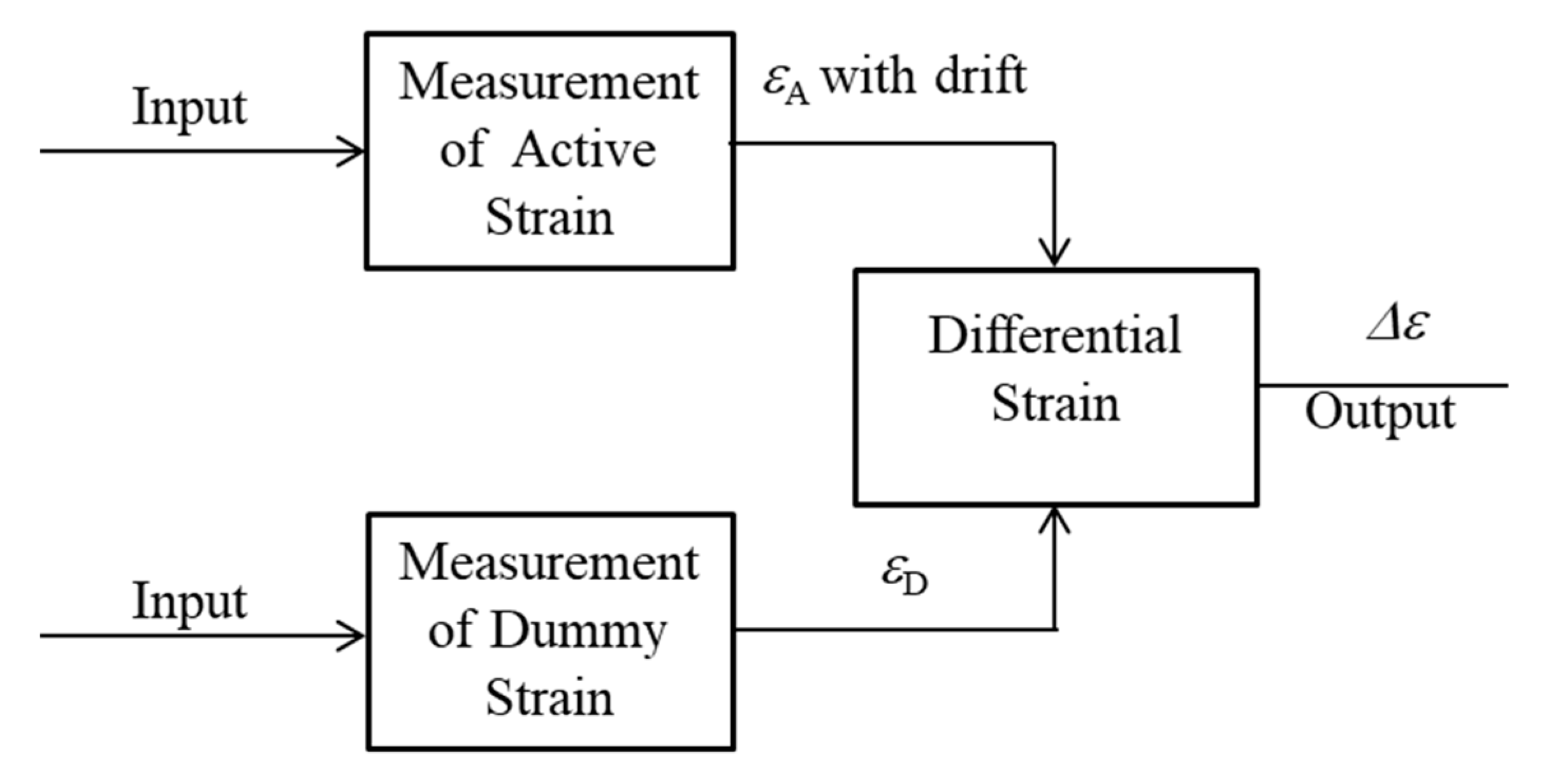
2.2. Concept of the ACSSM with an Active Dummy Circuit Method

To observe the thickness reduction by corrosion of the test piece based on the strain measurement, accurate measurement is necessary, because the thickness reduction of the test piece in a short time period is generally ≤5 × 10⁻⁶ m.
Environmental factors, such as temperature variations, during measurement affect not only the test piece and sensor, but also device elements such as the operation amplifier, causing measurement drift.
Therefore, to observe small thickness reductions caused by corrosion, the active dummy circuit method was proposed. In this study, the active dummy method consists of not only active and dummy sensors but also active and dummy circuits for strain measurement. Figure 2 shows the concept of ACSSM with an active dummy method. The active output (εΑ) of an active gauge of an active circuit included the drift of the sensor from environmental factors. Therefore, the dummy output (εD) of the dummy gauge of the active circuit was used to eliminate the effects of environmental factors during the measurement.
The output of the dummy circuit is the difference between the outputs of active and dummy strain gauges; to eliminate the drift from the circuit itself, the output of the dummy circuit was used. The strain (Δε) was finally obtained as the difference between the output of the active and dummy circuits with the difference circuit. In the study, two active and two dummy strain gauges were employed to enhance the resolution of the measured strain.

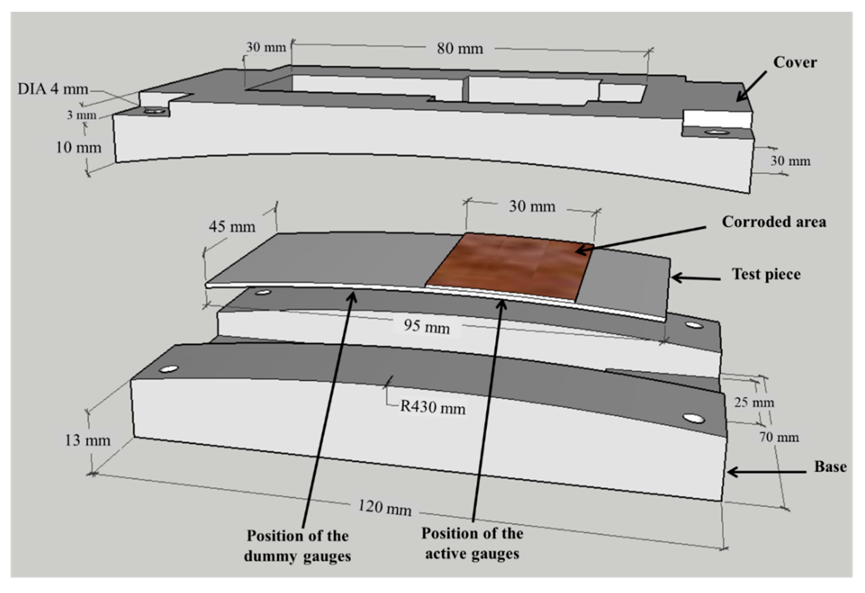
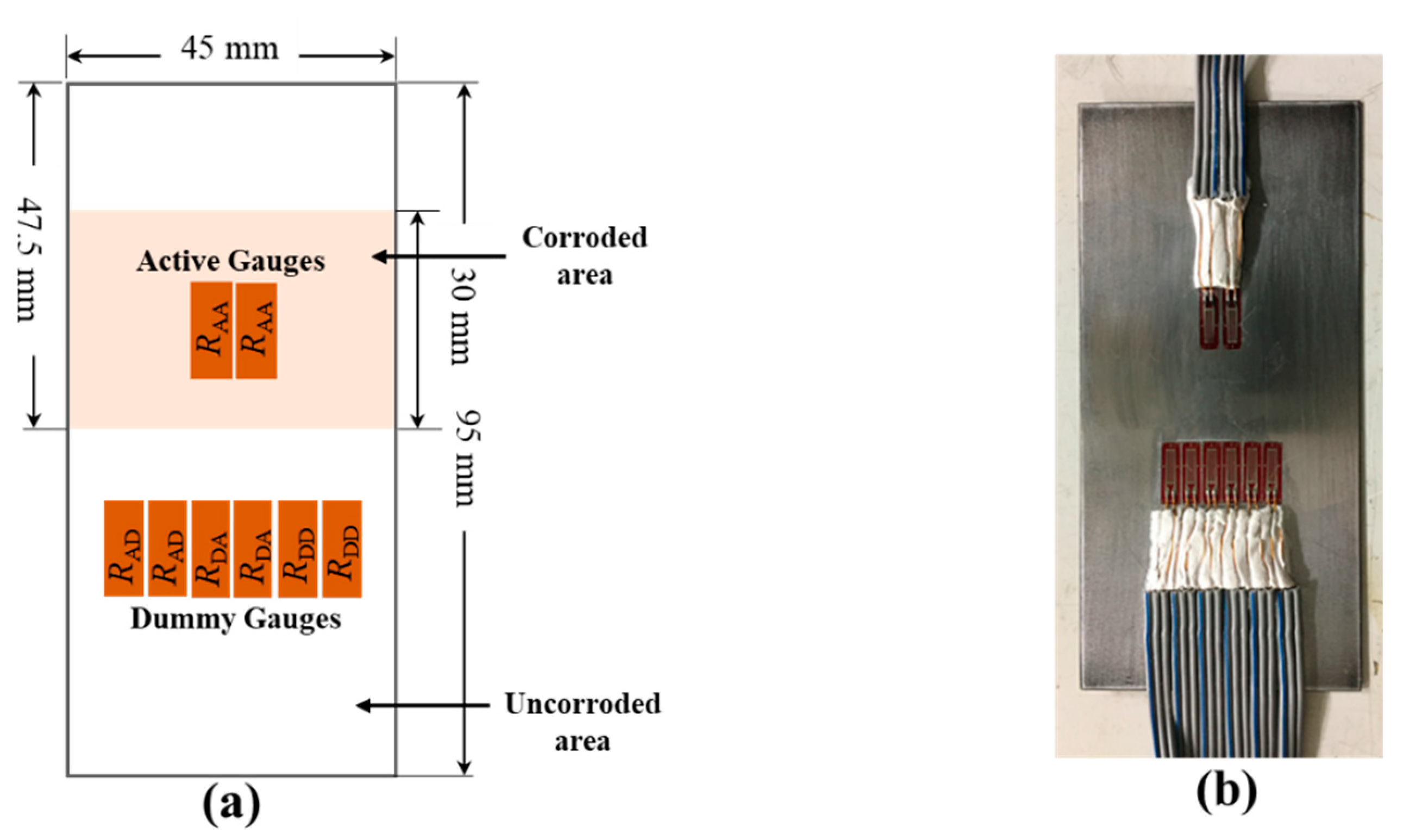
2.3. Design of the ACSSM with an Active Dummy Method

As mentioned above, two active and two dummy strain gauges were employed. The gain of the strain measurement circuit using the gain resistor (RG) of 4 Ω with the active dummy method was 12,500. The relationship between the voltage and strain in the master curve was measured [31]. Using the RG of 4 Ω, relationship between the strain and voltage was linear, following the equation Δε = –11 + 27 ΔV, where ΔV is the output voltage of the strain measurement circuit before it is converted to Δε. The slope of the equation was used to convert the output voltage of the circuit to strain, which was 27 × 10−6 ε for 1 V.

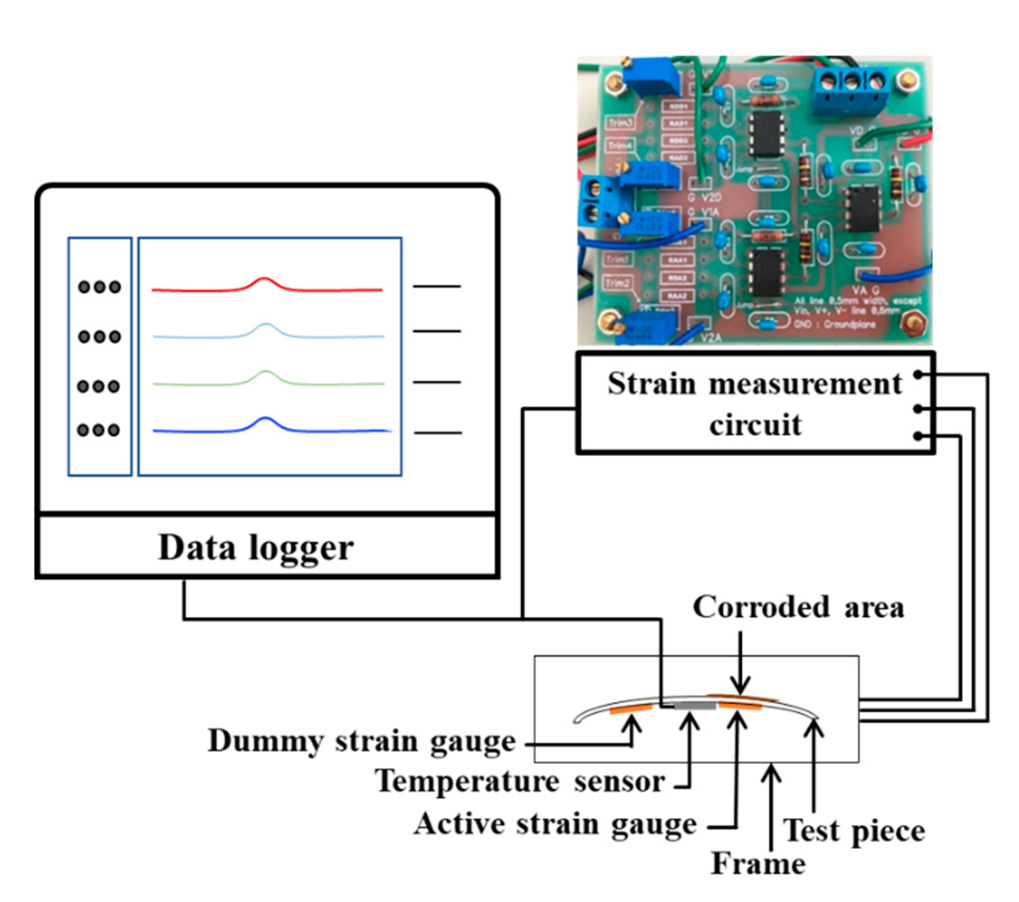
2.4. Experimental Setup for Dry-Wet Measurement by ACSSM

The test piece of the sensor is 95 mm in length, 45 mm in width, and 0.5 mm in thickness, made of low-carbon steel, has a corroded area of 1350 mm2, as shown in Figure 3. The ACSSM device comprises a base and cover with ρ = 430 mm, as in reference [30]. The test piece is placed in the apparatus and the edges of the test piece are fixed.
Eight strain gauges were attached to the back side of the test piece in the configuration as shown in Figure 4. The two active gauges (RAA) of the active circuit were attached beneath the corroded area and two dummy (RAD) gauges of the active circuit are attached beneath the uncorroded area. In the dummy circuit, four strain gauges (RDA and RDD), equal to the number of strain gauges in the active circuit, were used and attached beneath the non-corroded area.
Δε between εA and εD is used to evaluate the thickness reduction from the corrosion. The strain measurement circuit having an active circuit, dummy circuit and differential circuit [31] were fabricated by authors. As strain gauge, FLA-5-11 (Tokyo Sokki, Tokyo, Japan), the ACSSM were used. The input voltage of bridge circuits of active and dummy circuits was 3 Volt.
Figure 5 shows the experimental set-up of the dry-wet condition using strain gauges. The data logger GL7000 (Graphtec, Yokohama, Japan) monitors the output voltage from the active, dummy, and differential circuits every 10 min and measures the temperature simultaneously with a thermocouple. Using the relationship between strain and voltage given in Section 2.3 and the relationship between strain and thickness using the mechanical calculation in [15], Δh = 0.86 Δε × 10−6 m, Δh is obtained with Equation (2).
In the experiment, a 5.0 wt % NaCl (salt) solution is periodically applied to the test piece in the sensor under dry-wet conditions. The experiment is performed in two stages: the initial measurement before spraying the salt solution to investigate the compensation of environmental factors, and the dry-wet condition with sprayed salt solution. To discuss thickness reduction based on the strain measurement, several specimens of test piece material as coupon were prepared and periodically sprayed with 5.0 wt % NaCl solution. The test piece and coupons were sprayed once a day using around 3.75 mL of 5.0 wt % NaCl solution.

3. Results and Discussion

Figure 6 shows the experiment results under dry-wet condition using ACSSM for 15 days before salt solution is applied. The results indicate the effects and the compensation of environmental factors on the signal. The εA follows the temperature signal of the test piece (TTP) and has the same tendency as the εD. TTP varies over approximately 0 to 20°C for εA around 100 × 10−6 ε; the drift is 5 × 10⁻⁶ ε/°C. Despite using the active and dummy strain gauge method. Meanwhile, Δε is more constant around 25 × 10−6 ε with a drift of is 1.25 × 10⁻⁶ ε/°C. This corresponds to a 75% decreased in drift from environmental factors. The ACSSM measurement system with the active dummy circuit method is therefore robust against environmental factors, such as temperature variations, during measurement.
Figure 7 shows the results of dry-wet exposure with ACSSM. Three stages are observed in the result. Stage I is the initial condition for 15 days before spraying with salt water. This stage is shown as Figure 6. Stage II is the condition after spraying salt water, in which corrosion products are generated. Δε shows a negative trend, indicating that the test piece thickness is increased by the corrosion products. Stage III is the condition of further corrosion progression, which causes thickness reduction by corrosion of the corrosion products. Δε shows a positive trend. According to Equation (2), this indicates that the test piece thickness is decreased by corrosion, including that of corrosion products. As the corrosion of the test piece continues after salt-solution spraying, the variations of Δε become large. It happened because of corrosion progress, two RAA under the corroded area and the two RDD under non-corroded area show different behavior, although these show the same behavior in Stage I. Compared to RDD, RAA under the corrosion product react slowly to temperature variations, because the corrosion product functions as a thermal insulator. Therefore, the difference in the balance of the measurement system bridge circuit is large, yielding a larger variation of Δε.
Δε is converted to Δh, and Δh is applied by a moving average analysis using intervals of 200 data sets to obtain the signal more clearly without deleting the trends of each stage. Moreover, Δh is moved to zero value become Δhoffset (10−6 m). The result is shown in Figure 8. Simultaneously, the test piece results are obtained, and the thickness reductions of the specimens calculated by the mass loss are indicated in Figure 8. The thickness reductions show good correlation that measured with ACSSM. However, the evaluation errors between the result measured with ACSSM and the thickness of specimen as shown in Table 1 were 14.5 × 10⁻⁶ m. This error is calculated using the average of the last four data points from each method.
Figure 9 shows photograph of the evolution of the corrosion product on the test piece for 83 days. After spraying salt solution, the corrosion of the test piece progresses. These pictures are similar to the appearance of the specimen surfaces at the same times.
Although ACSSM can measure only the thickness reduction of the test piece, a schematic of the mechanism of corrosion behavior measured with ACSSM was illustrated. It is shown in Figure 10. Stage I is the initial stage, with no corrosion product on the surface of the test piece and constant Δε.
In stage II, a tight corrosion product would be generated. Δε shows a slight decreasing tendency because of this tight corrosion product, indicating that the test piece thickness would be increased by the tight corrosion product. The increased thickness of the test piece measured with ACSSM is approximately 43 × 10−6 m for 25 days. In stage III, the corrosion of the test piece would yield a porous structure with continued corrosion, and the test piece thickness is decreased because the porous structure of corrosion product receives bending moment. The thickness reduction of the test piece measured with ACSSM is approximately 111 × 10−6 m in 43 days. As shown above, the monitoring with the ACSSM needs sufficient time after stage III to measure thickness reduction of the test piece.

4. Conclusions

An ACSSM with an active dummy method, proposed by authors, was used for experimentation with the dry-wet method in long-term monitoring. The conclusions of this study are as follows:
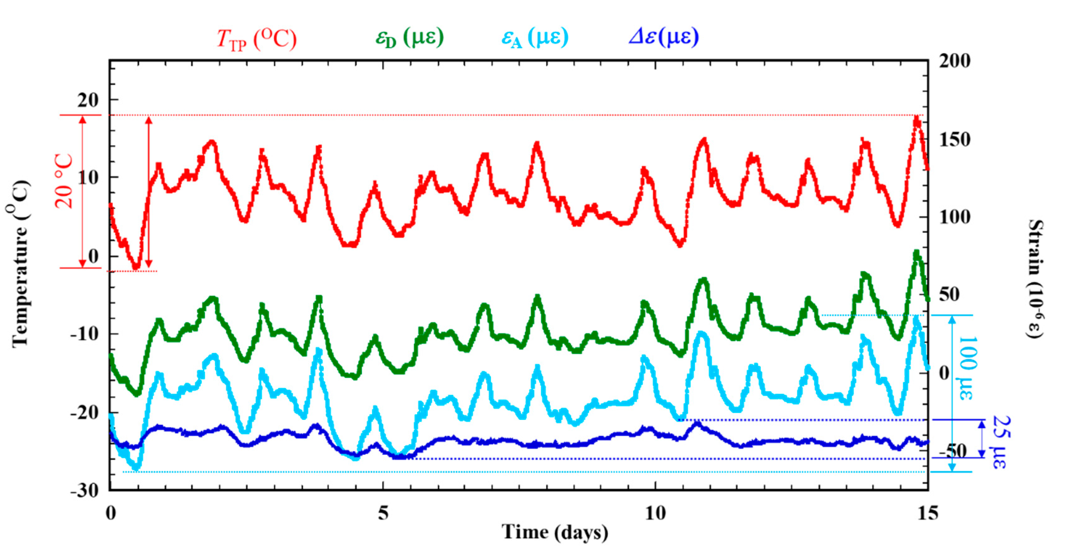
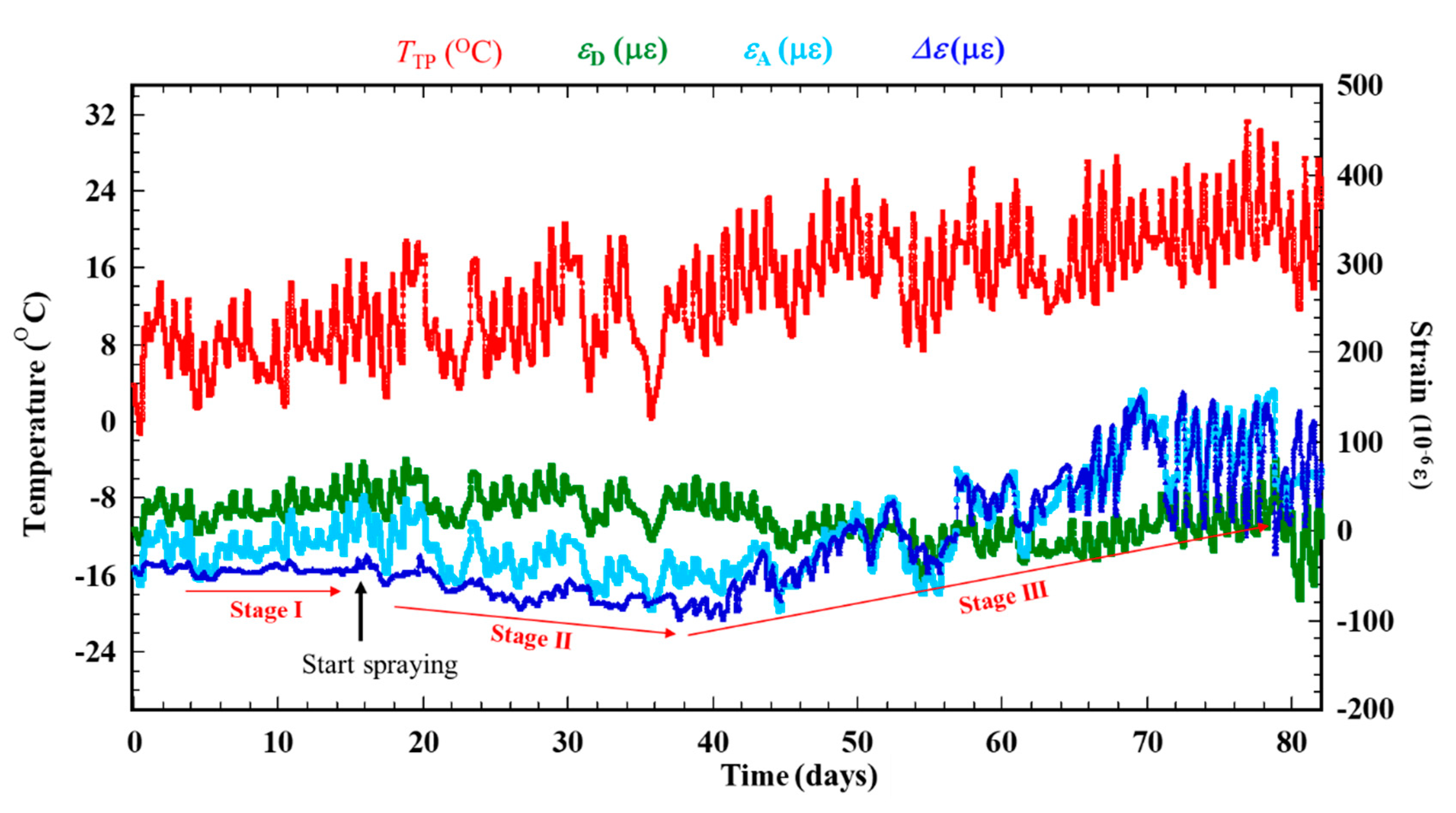
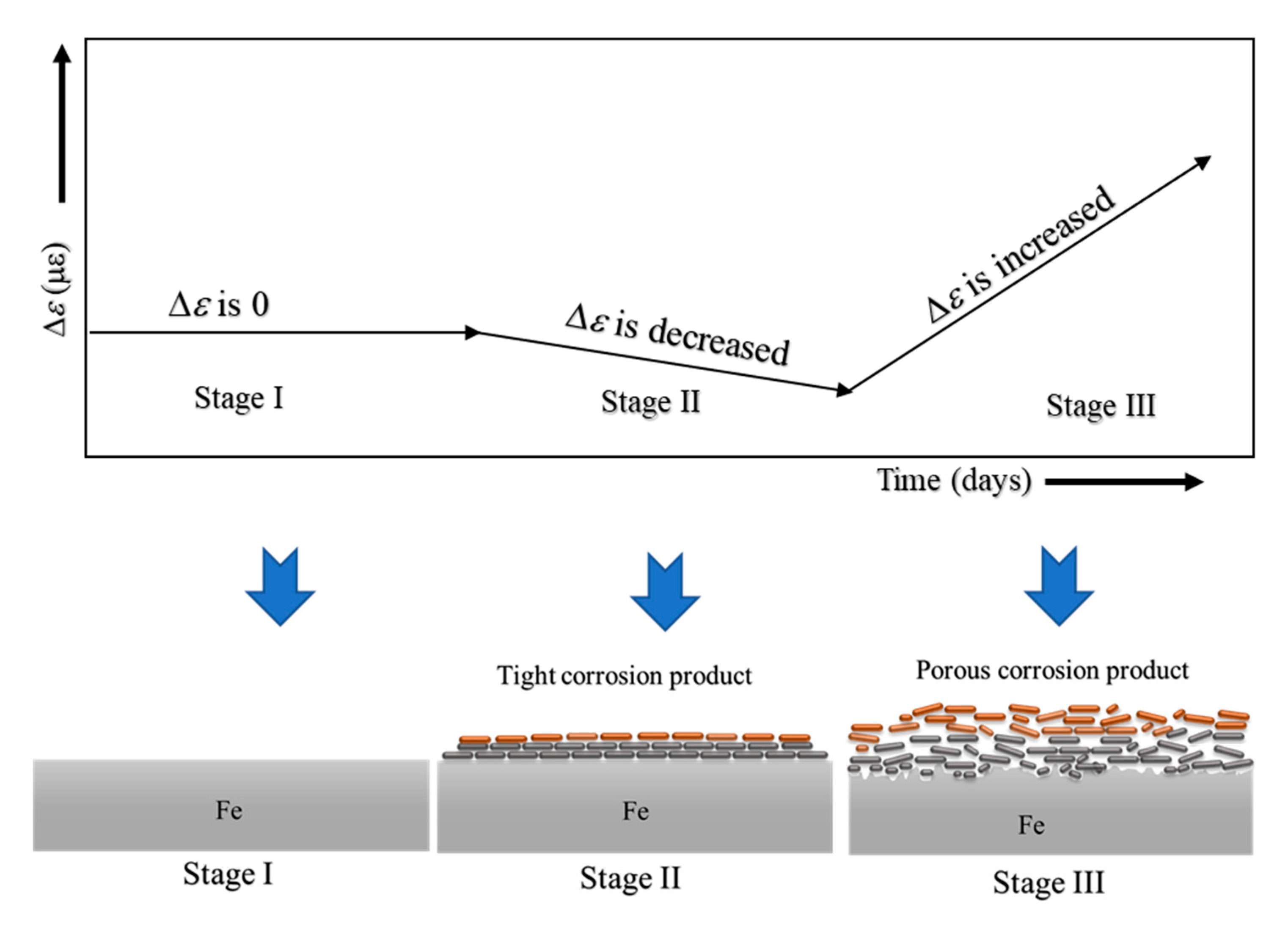
  • In stage I of the experiment, Δε had a relative constant signal, with drift decreasing from 5 × 10⁻⁶ ε/°C to 1.25 × 10⁻⁶ ε/°C under temperature variations.
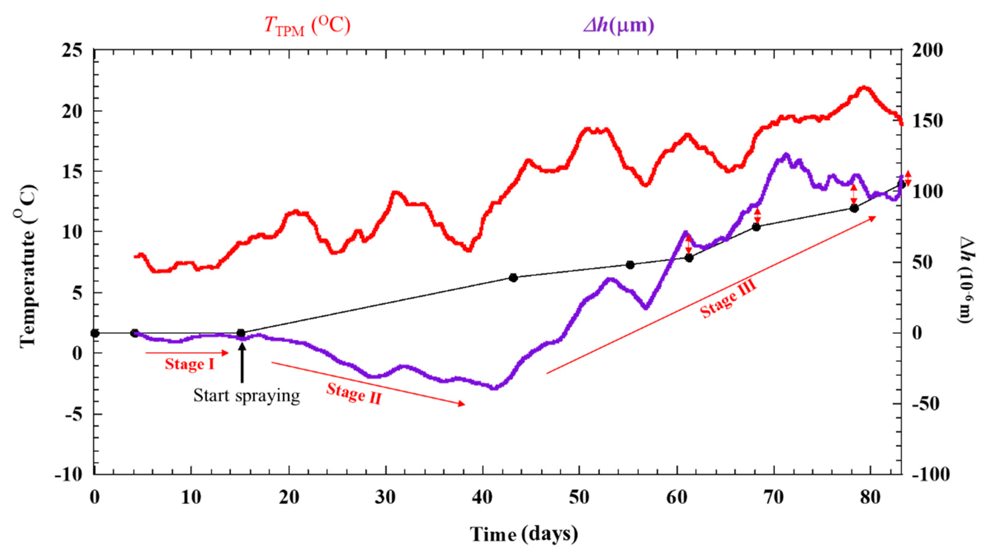
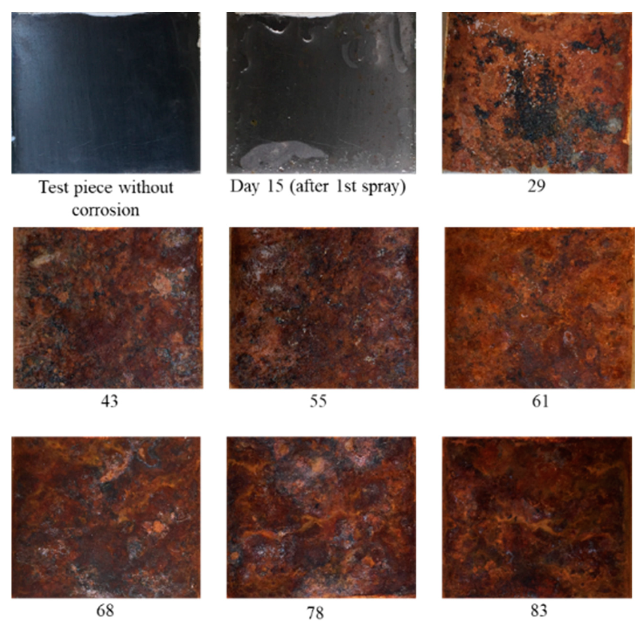
  • In stage II, Δε showed a negative trend, indicating the increased thickness of the test piece measured by ACSSM. This was attributed to the tight corrosion product formed on the test piece measured by ACSSM.
  • In stage III, showed a positive trend because the produced corrosion product was porous. The accuracy of h was determined from the thickness reduction of the coupons. Thus, ACSSM can be used for atmospheric corrosion monitoring in the field.
  • The sensor applies for atmospheric corrosion, for general corrosion. The sensor can be measured the strain that has relation with the thickness of test piece and finally we can calculate the corrosion rate. The local corrosion condition in the test piece of the sensor affects the accuracy of the corrosion rate estimation. This problem might be considered in a future study.

Author Contributions

Conceptualization, H.K.; methodology, S.O. and N.P.; software, N.K.; validation, H.K., N.K. and Y.K.; formal analysis, N.K. and N.P.; investigation, N.P.; resources, N.K.; data curation, Y.K. and S.O.; writing—original draft preparation, N.P.; writing—review and editing, N.K., Y.K. and N.P.; visualization, S.O.; supervision, N.K.; project administration, N.K.; funding acquisition, N.K.

Funding

This work was supported by a Grant-in-Aid for Scientific Research (B) JSPS KAKENHI Grant No. 16H03132 and Yokohama National University.

Acknowledgments

The authors would like to thank to the Indonesian Directorate General of Higher Education for their financial support of the author’s study.

Conflicts of Interest

The authors declare there is no conflict of interest. The supporters did not have a role in the design of the study; in the collection, analyses, and interpretation of data; in the writing of the manuscript, or in the decision to publish the results.

Nomenclature

ρRadius of curvature of the test piece (m)
hTest piece in thickness (m)
εStrain in the test piece (-)
Centre angle of curvature of the test piece (o)
ΔhChange of thickness of the test piece (m)
h’Test piece in thickness due to the corrosion (m)
εAStrain of active circuit (×10−6 ε)
εDStrain of dummy circuit (×10−6 ε)
ΔεDifference in strain in the test piece due to the corrosion (×10−6 ε) Difference in strain between εA and εD (×10−6 ε)
EYoung’s modulus of the test piece (Pa)
σyYield stress of the test piece (Pa)
VINInput voltage for bridge circuit (V)
RAAResistance of active gauge for active circuit (Ω)
RDAResistance of dummy gauge for active circuit (Ω)
RADResistance of active gauge for dummy circuit (Ω)
RDDResistance of dummy gauge for dummy circuit (Ω)
ΔVDifferent output voltage of active and dummy circuit (V)
TTPTemperature of test piece (°C)
TTPMTemperature of test piece after applied moving average analysis (°C)
ΔhwActual thickness from weight analysis of coupons (×10−6 m)

References

  1. Morcillo, M.; De Fuente, D.; Diaz, I.; Cano, H. Atmospheric corrosion of mild steel. Rev. Metal. 2011, 47, 426–444. [Google Scholar] [Green Version]
  2. Song, H.W.; Saraswathy, V. Corrosion monitoring of reinforced concrete structures—A review. Int. J. Electrochem. Sci. 2007, 1–28. [Google Scholar]
  3. Wen, X.; Bai, P.; Luo, B.; Zheng, S.; Chen, C. Review of recent progress in the study of corrosion products of steels in a hydrogen sulphide environment. Corros. Sci. 2018, 139, 124–140. [Google Scholar]
  4. Ahmad, S. Reinforcement corrosion in concrete structures, its monitoring and service life prediction—A review. Cem. Concr. Compos. 2003, 25, 459–471. [Google Scholar] [CrossRef]
  5. Alamin, M.; Tian, G.Y.; Andrews, A.; Jackson, P. Corrosion detection using low-frequency RFID technology. Insight-Non-Destr. Test. Cond. Monit. 2012, 54, 72–75. [Google Scholar]
  6. Zhang, H.; Yang, R.; He, Y.; Tian, G.Y.; Xu, L.; Wu, R. Identification and characterization of steel corrosion using passive high frequency RFID sensors. Measurement 2016, 92, 421–427. [Google Scholar]
  7. Zhang, J.; Tian, G.Y.; Marindra, A.M.J.; Sunny, A.I.; Zhao, A.B. A review of passive RFID tag antenna-based sensors and systems for structural health monitoring applications. Sensors 2017, 17, 265. [Google Scholar] [CrossRef]
  8. Yasri, M.; Gallee, F.; Lescop, B.; Diler, E.; Thierry, D.; Rioual, S. Passive wireless sensor for atmospheric corrosion monitoring. In Proceedings of the 8th European Conference on Antennas and Propagation (EuCAP), The Hague, The Netherlands, 6–11 April 2014; pp. 2945–2949. [Google Scholar]
  9. Perveen, K.; Bridges, G.E.; Bhadra, S.; Thomson, D.J. Corrosion potential sensor for remote monitoring of civil structure based on printed circuit board sensor. IEEE Trans. Instrum. Meas. 2014, 63, 2422–2431. [Google Scholar] [CrossRef]
  10. Almubaied, O.; Chai, H.K.; Islam, M.R.; Lim, K.; Tan, C.G. Monitoring corrosion process of reinforced concrete structure using FBG strain sensor. IEEE Trans. Instrum. Meas. 2017, 66, 2148–2155. [Google Scholar] [CrossRef]
  11. Tan, C.H.; Adikan, F.R.M.; Shee, Y.G.; Yap, B.K. Non-destructive fiber Bragg grating based sensing system: Early corrosion detection for structural health monitoring. Sens. Actuators A Phys. 2017, 268, 61–67. [Google Scholar] [CrossRef]
  12. Hassan, M.R.A.; Bakar, M.H.A.; Dambul, K.; Adikan, F.R.M. Optical-based sensors for monitoring corrosion of reinforcement rebar via an etched cladding Bragg grating. Sensors (Basel) 2012, 12, 15820–15826. [Google Scholar] [CrossRef] [PubMed]
  13. Hu, W.; Ding, L.; Zhu, C.; Guo, D.; Yuan, Y.; Ma, N.; Chen, W. Optical fiber polarizer with Fe-C film for corrosion monitoring. IEEE Sens. J. 2017, 17, 6904–6910. [Google Scholar]
  14. Chen, W.; Dong, X. Modification of the wavelength-strain coefficient of FBG for the prediction of steel bar corrosion embedded in concrete. Opt. Fiber Technol. 2012, 18, 47–50. [Google Scholar] [CrossRef]
  15. Al Handawi, K.; Vahdati, N.; Rostron, P.; Lawand, L.; Shiryayev, O. Strain based FBG sensor for real-time corrosion rate monitoring in pre-stressed structures. Sens. Actuator B 2016, 236, 276–285. [Google Scholar] [CrossRef]
  16. Dara, T.; Shinohara, T.; Umezawa, O. The Behavior of corrosion of low carbon steel affected by corrosion product and Na2SO4 concentration under artificial rainfall test. Zairyo Kankyo 2016, C-114, 298–302. [Google Scholar]
  17. Monsada, A.M.; Margarito, T.; Milo, L.C.; Casa, E.P.; Zabala, J.V.; Maglines, A.S.; Basilia, B.A.; Harada, S.; Shinohara, T. Atmospheric corrosion exposure study of the Philippine historical all-steel Basilica. Zair. Kankyo 2016, C-107, 267–270. [Google Scholar]
  18. Mansfeld, F.; Jeanjaquet, S.L.; Kendig, M.W.; Roe, D.K. A new atmospheric corrosion rate monitor development and evaluation. Atmos. Environ. 1986, 20, 1179–1192. [Google Scholar]
  19. Ridha, M.; Fonna, S.; Huzni, S.; Supardi, J.; Ariffin, A.K. Atmospheric corrosion of structural steels exposed in the 2004 tsunami-affected areas of Aceh. IJAME 2013, 7, 1014–1022. [Google Scholar] [CrossRef]
  20. Parson, N.; Khamsuk, P.; Sorachot, S.; Khonraeng, W.; Wongpinkaew, K.; Kaewkumsai, S.; Pongsaksawad, W.; Viyanit, E.; Chianpairot, A. Atmospheric corrosion of structural steels in Thailand Tropical Climate. Zairyo Kankyo 2016, C-108, 271–274. [Google Scholar]
  21. Lien, L.T.H.; Hong, H.L.; San, P.T.; Hieu, N.T.; Nga, N.T.T. Atmospheric corrosion of carbon steel and weathering steel—Relation of corrosion and environmental factors. Zairyo Kankyo 2016, C-110, 280–284. [Google Scholar]
  22. Odara, T.; Tahara, A.; Dara, T. Atmospheric corrosion behaviors of steels in Japan. Zairyo Kankyo 2016, C-111, 285–288. [Google Scholar]
  23. Shitanda, I.; Okumura, A.; Itagaki, M.; Watanabe, K.; Asano, Y. Screen printed atmospheric corrosion monitoring sensor based on electrochemical impedance spectroscopy. Sens. Actuators B Chem. 2009, 139, 292–297. [Google Scholar]
  24. Li, C.; Ma, Y.; Li, Y.; Wang, F. EIS monitoring study of atmospheric corrosion under variable relative. Corros. Sci. 2010, 52, 3677–3686. [Google Scholar] [CrossRef]
  25. Thee, C.; Dong, J.; Ke, W. Corrosion monitoring of weathering steel in a simulated coastal-industrial environment. Int. J. Environ. Chem. Ecol. Eng. 2015, 9, 587–593. [Google Scholar]
  26. Luo, J. Corrosion of the galvanized steel bolts of overhead catenary system in the tunnel areas. Proc. JSCE Mater Environ. 2016, 293–297. [Google Scholar]
  27. Hu, W.; Cai, H.; Yang, M.; Tong, X.; Zhou, C.; Chen, W. Fe-C-coated fiber Bragg grating sensor for steel corrosion monitoring. Corros. Sci. 2011, 53, 1933–1938. [Google Scholar]
  28. Zang, N.; Chen, W.; Zheng, X.; Hu, W.; Gao, M. Optical sensor for steel corrosion monitoring based on etched Fiber Bragg Grating sputtered with iron film. IEEE Sens. J. 2015, 15, 3511–3556. [Google Scholar]
  29. Ke, W.; Dong, J.H.; Chen, W. Corrosion evolution of steel simulated of SO2 polluted coastal atmospheres. Zair. Kankyo. 2016, C-112, 289–292. [Google Scholar]
  30. Kasai, N.; Hiroki, M.; Yamada, T.; Kihira, H.; Matsuoka, K.; Kuriyama, Y.; Okazaki, S. Atmospheric corrosion sensor based on strain measurement. Meas. Sci. Technol. 2016, 28, 015106. [Google Scholar]
  31. Purwasih, N.; Kasai, N.; Okazaki, S.; Kihira, H. Development of amplifier circuit by active dummy method for atmospheric corrosion monitoring on steel. Metals 2018, 8, 1–12. [Google Scholar]
  32. Abbas, Y.; Nutma, J.S.; Olthuis, W.; Van Den Berg, A. Corrosion monitoring of reinforcement steel using galvanostatically induced potential transients. IEEE Sens. J. 2016, 16, 693–698. [Google Scholar]
  33. Stroosnijder, M.F.; Brugnoni, C.; Laguzzi, G.; Luvidi, L.; De Cristofaro, N. Atmospheric corrosion evaluation of galvanised steel by thin layer activation. Corros. Sci. 2004, 46, 2355–2359. [Google Scholar]
  34. Portella, M.O.G.; Portella, K.F.; Pereira, P.A.M.; Inone, P.C.; Brambilla, K.J.C.; Cabussú, M.S.; Cerqueira, D.P.; Salles, R.N. Atmospheric corrosion rates of copper, galvanized steel, carbon steel and aluminum in the metropolitan region of Salvador, BA, Northeast Brazil. Proc. Eng. 2012, 42, 171–185. [Google Scholar] [CrossRef]
  35. Yadav, A.P.; Suzuki, F.; Nishikata, A.; Tsuru, T. Investigation of atmospheric corrosion of Zn using ac impedance and differential pressure meter. Electrochim. Acta 2004, 49, 2725–2729. [Google Scholar] [CrossRef]
  36. El-Mahdy, G.A. Atmospheric corrosion of copper under wet / dry cyclic conditions. Corro. Sci. 2005, 47, 1370–1383. [Google Scholar]
  37. Kiosidou, E.D.; Karantonis, A.; Sakalis, G.N.; Pantelis, D.I. Electrochemical impedance spectroscopy of scribed coated steel after salt spray testing. Corros. Sci. 2018, 137, 127–150. [Google Scholar]
  38. Dillmann, P.; Mazaudier, F.; Hoerle, S. Advances in understanding atmospheric corrosion of iron Rust characterisation of ancient ferrous artefacts exposed to indoor atmospheric corrosion. Corros. Sci. 2004, 46, 1401–1429. [Google Scholar]
Figure 1. The illustration of test piece in normal position and bending position: (a) non-corroded test piece, (b) corroded test piece. T(T’), N(N’), and O(O’) denote the tensile, neutral, and compressive planes. M(M’) denotes the bending moment.
Metals 09 00579 g001
Figure 2. The concept of ACSSM with an active dummy method.
Metals 09 00579 g002
Figure 3. Test piece and apparatus for atmospheric corrosion sensor using strain measurements (ACSSM). The test piece is inserted in the apparatus, which consists of a base and cover with the corroded area measuring 45 mm in length and 30 mm in width.
Metals 09 00579 g003
Figure 4. (a) Configuration of strain gauges in test piece with 1350 mm2 corroded area; the remaining area is not corroded. (b) Photograph of strain gauge attached to the test piece.
Metals 09 00579 g004
Figure 5. Experimental set-up of under dry-wet condition for ACSSM.
Metals 09 00579 g005
Figure 6. Compensation of thermal strain experiment signal (TTP) before under dry-wet condition are applied.
Metals 09 00579 g006
Figure 7. Result of a dry–wet cyclic exposure with ACSSM.
Metals 09 00579 g007
Figure 8. Result from dry-wet cyclic condition with ACSSM in 83 days after moving-average analysis and applying the offset value. The green line with double arrows indicated the differences of the last four dataset collected from the ACSSM and specimens.
Metals 09 00579 g008
Figure 9. Picture of corrosion evolution for 83 days of measurement. Strain are from the sprayed salt water, shown in the picture at Day 15.
Metals 09 00579 g009
Figure 10. Mechanism of corrosion behavior based on strain measurements.
Metals 09 00579 g010
Table 1. Error calculation between ACSSM and test specimens.
Δhw (10−6 m)Δhoffset (10−6 m)Error (10−6 m)
546814
759015
8811123
1051116
Average14.5

