

Enhanced Modal Participation Ratio-Based Structural Damage Identification: A New Filtering Approach Using Modal Assurance Criteria


Abstract
:1. Introduction
- ✓
- Determining the dynamic response of the building model investigated using a numerical method;
- ✓
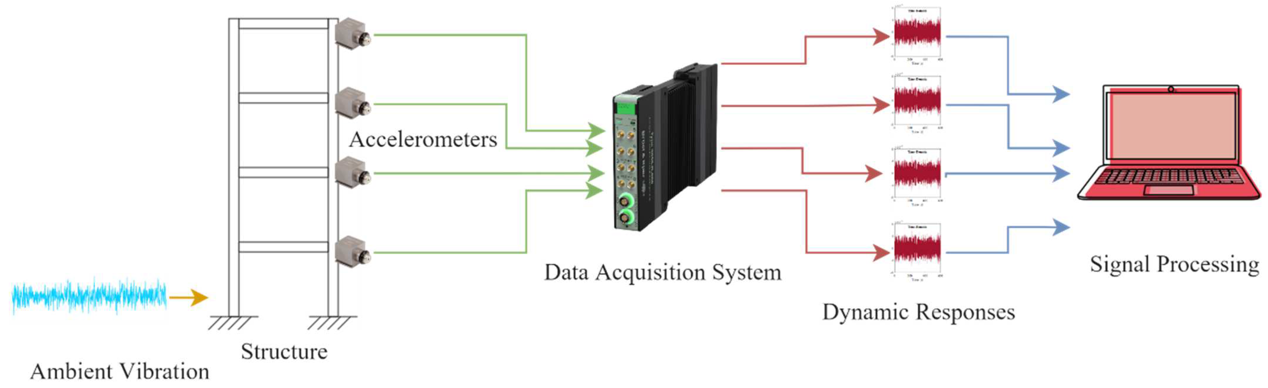
- Conducting an experimental test to obtain the dynamic responses and characteristics of a model;
- ✓
- Calculating the MPR values in light of numerical and experimental data;
- ✓
- Comparing numerical and experimental test results;
- ✓
- Developing a new filtering approach to get rid of user effects on MPR derivation;
- ✓
- Evaluating the damage detection method in case of using a new filtering approach for experimental data.
2. Methodology
2.1. Dynamic Response
2.2. Modal Participation Ratio (MPR) Derivation
2.2.1. Filtering
Bandpass Filtering
MAC Rejection Level
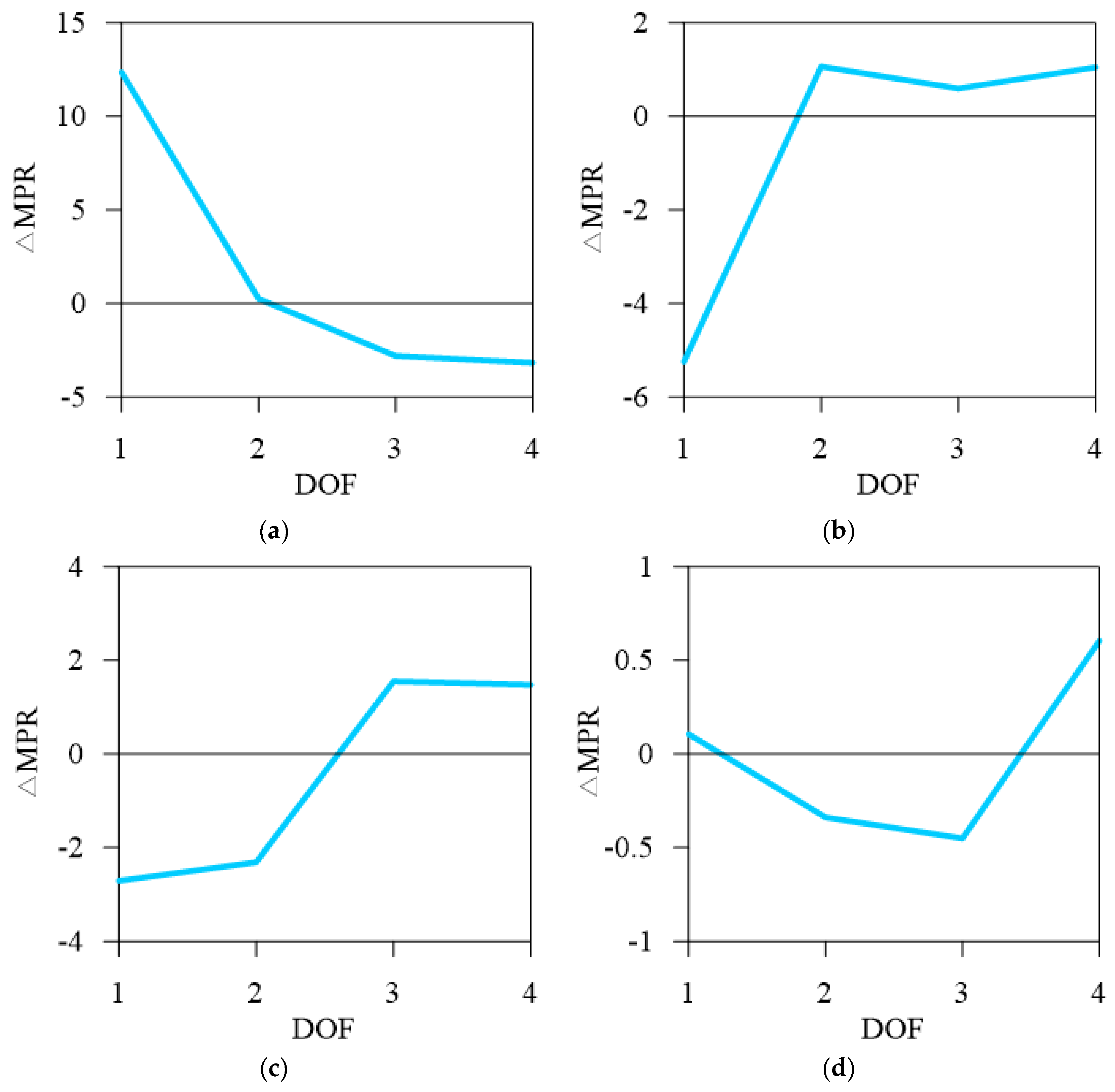
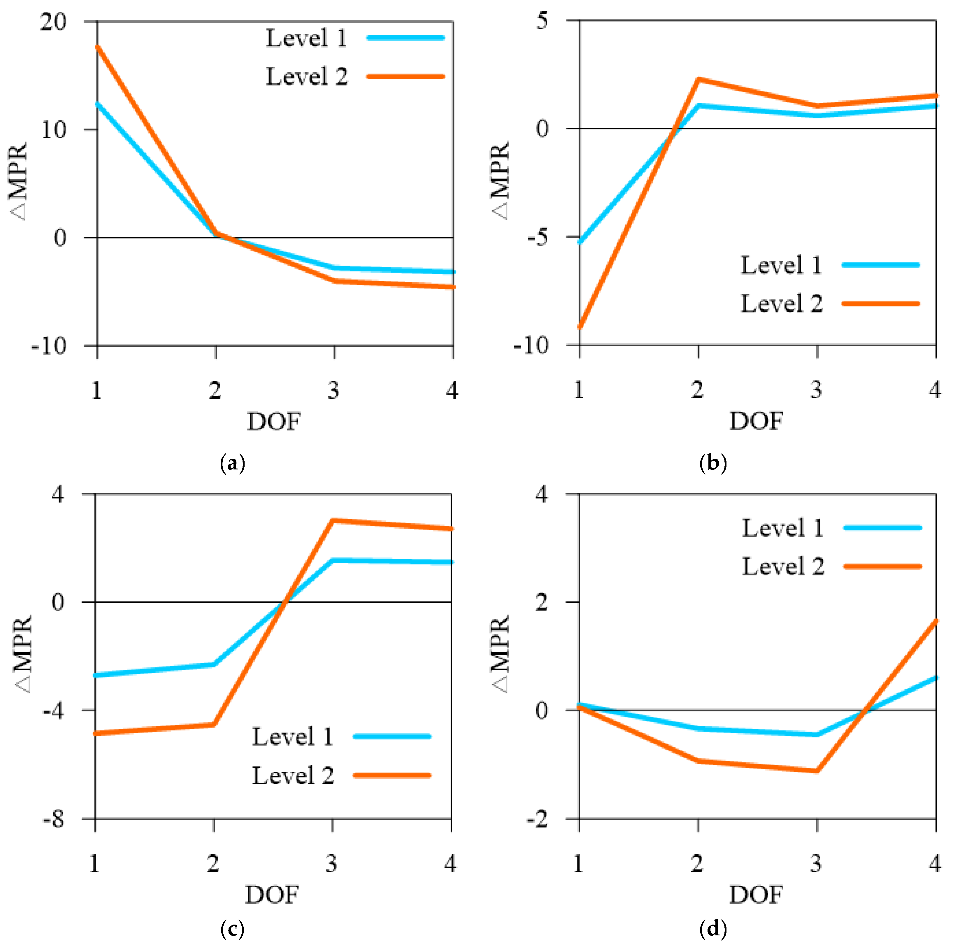
2.3. MPR Variation
3. Case Study
3.1. Model Design
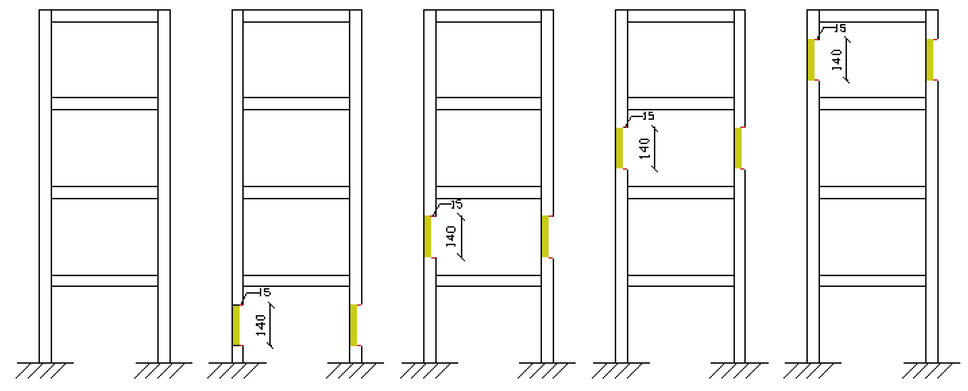
3.2. Damage Scenarios
3.3. Numerical Study
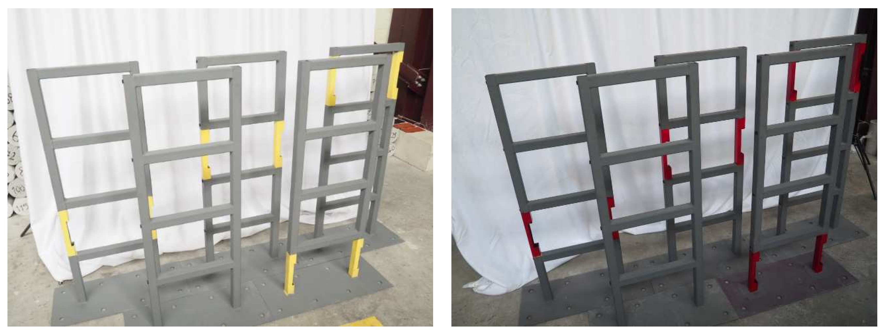
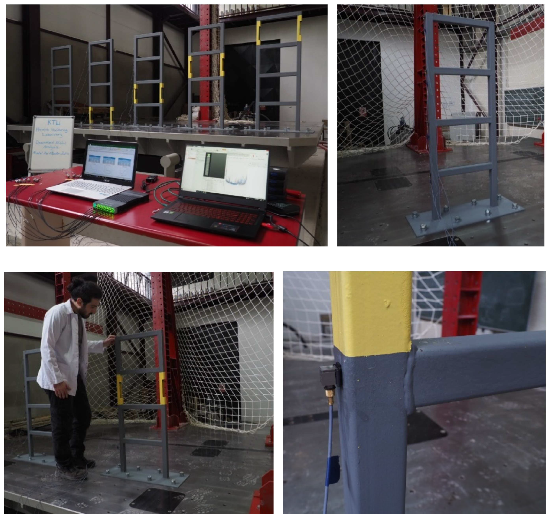
3.4. Experimental Study
4. Conclusions
- ✓
- The natural frequencies decreased as a result of introduced damage to building model. It should be noted that it is expected to see a decrease in natural frequency upon damage in the system, considering its effect on stiffness, alterations in mass distribution, damping effects and loss of structural integrity. It should be stated, however, that the natural frequencies increased after the introduction of the damage at fourth story. Damping ratios generally increased in the case of damaged models. However, a favorable interpretation was not possible for damage identification.
- ✓
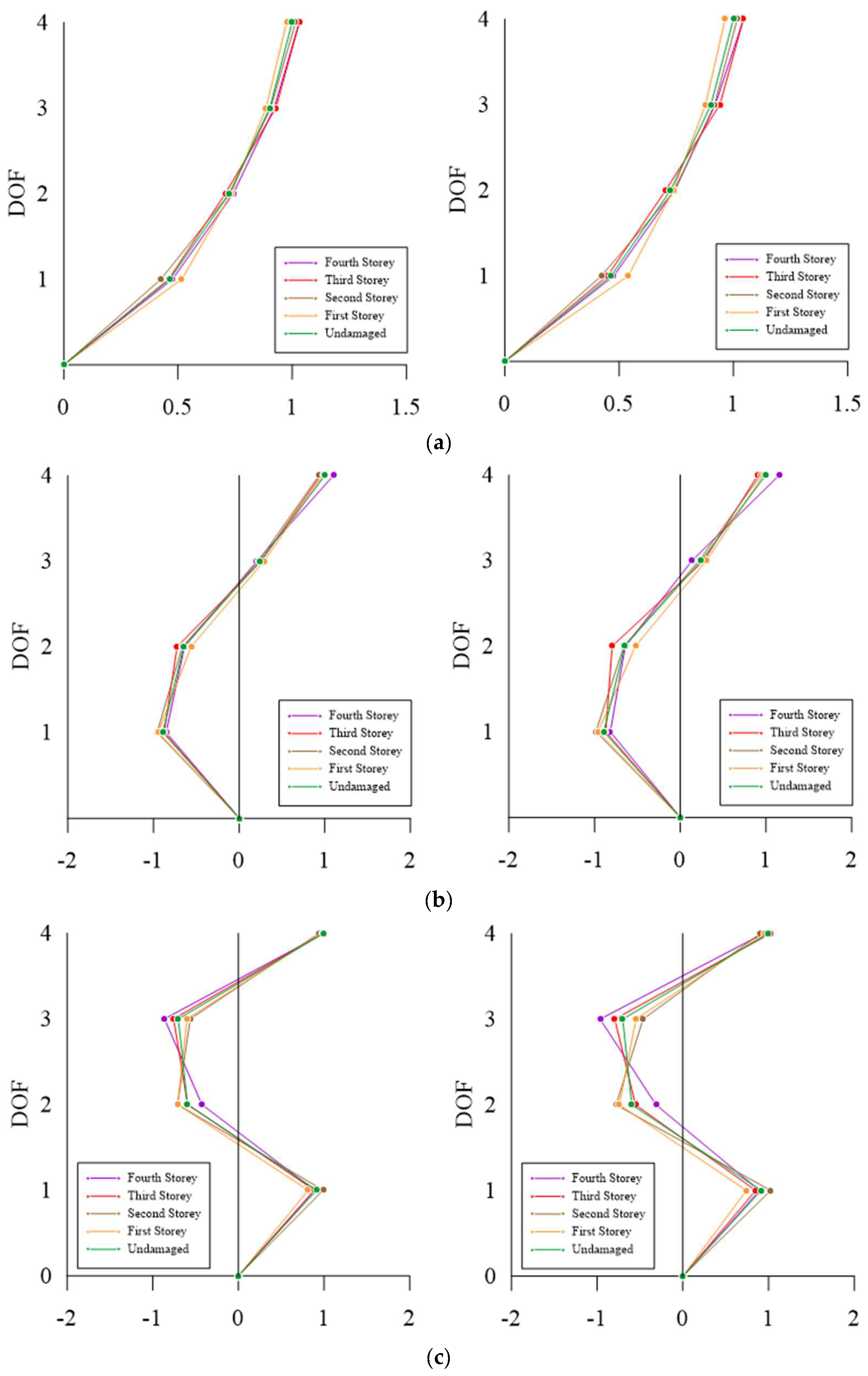
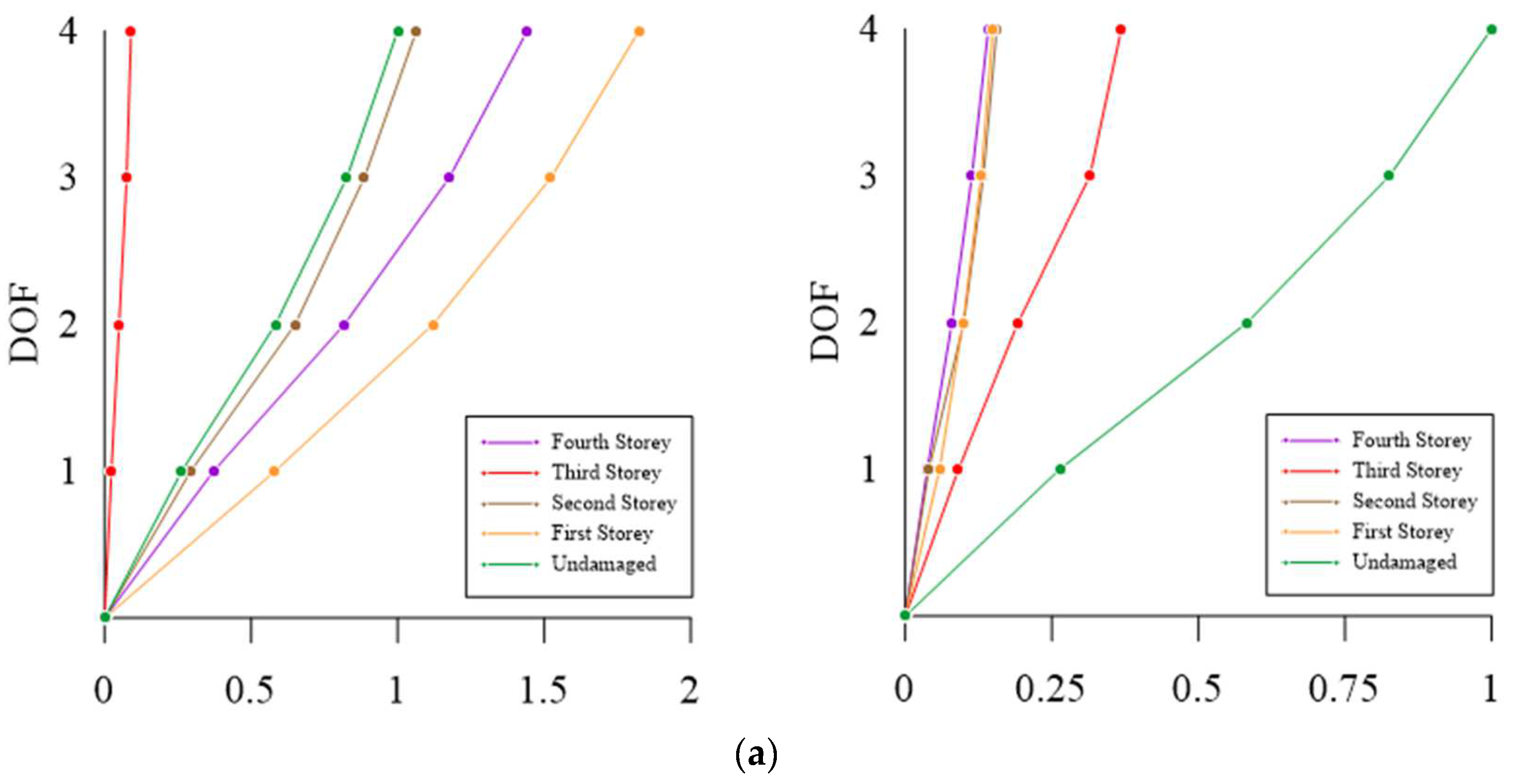
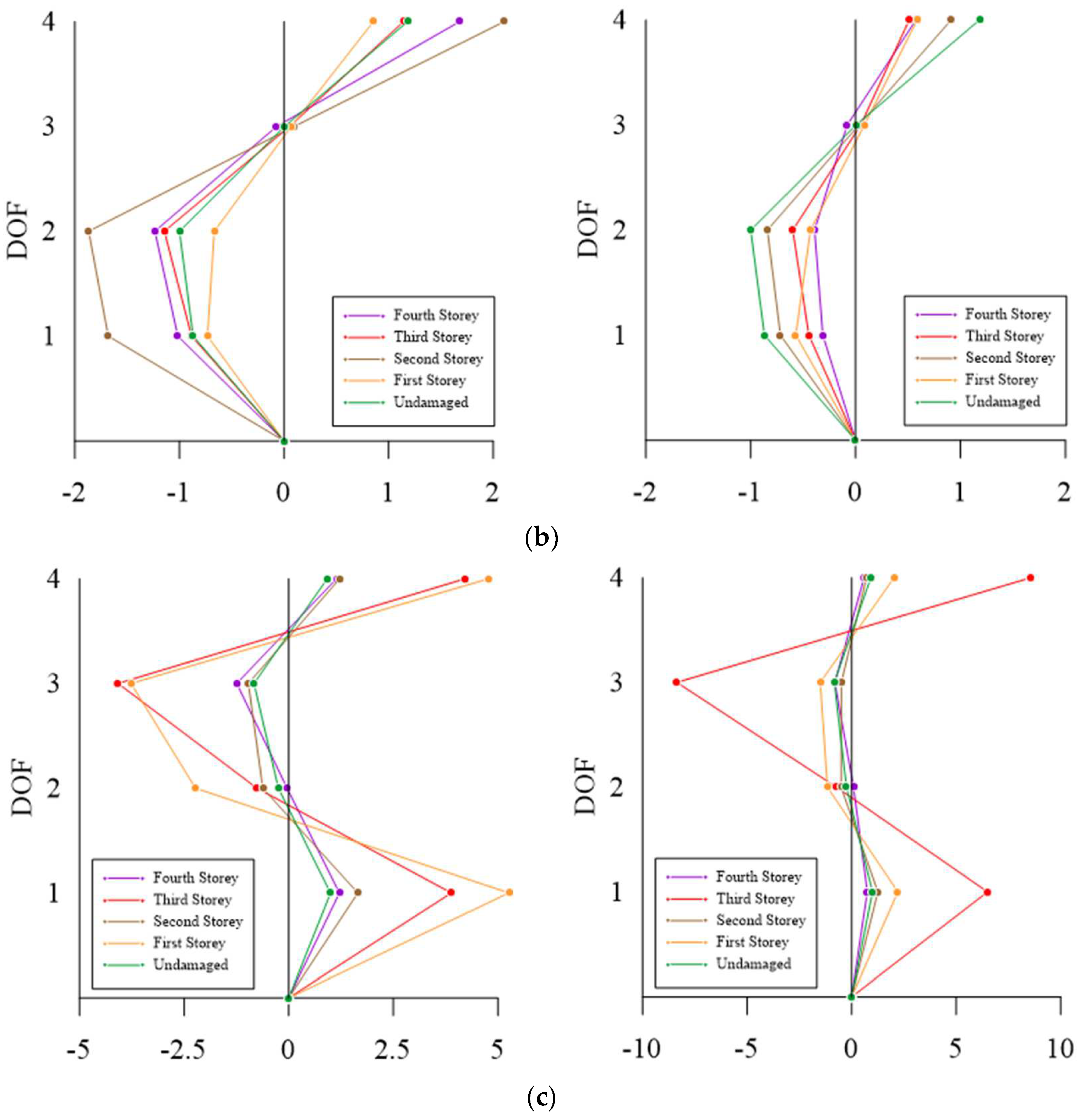
- Further study is required for mode shape variation, since the changes in nodal displacements are not observable due to the introduced damage scenarios. The relation between nodal displacements within the mode shape is required. However, using multiple parameters along with mode shape for detecting the damage presence, severity and location can be more effective.
- ✓
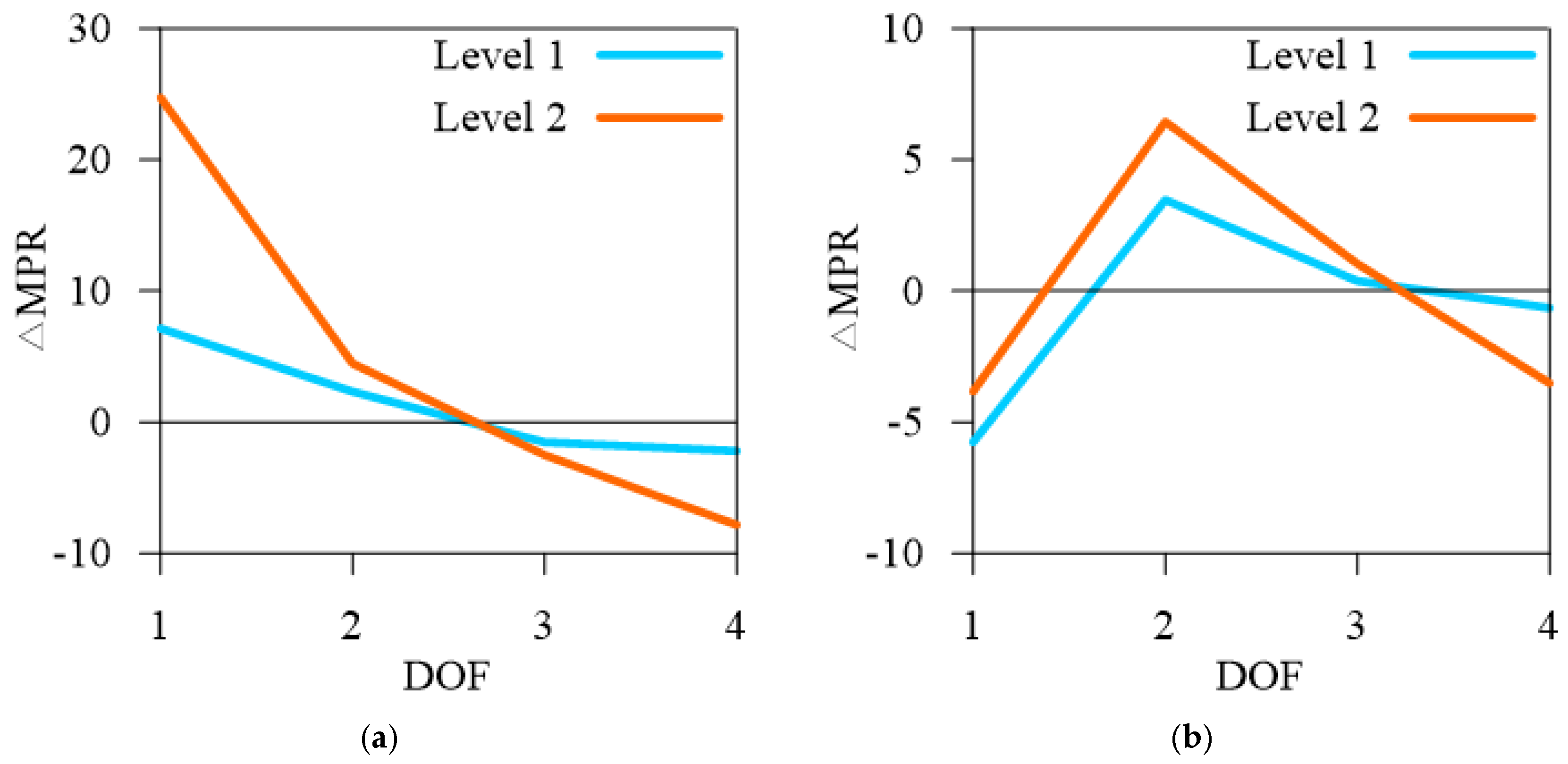
- The numerical and experimental results indicated that the values were highly capable of detecting the damage location and damage severity.
- ✓
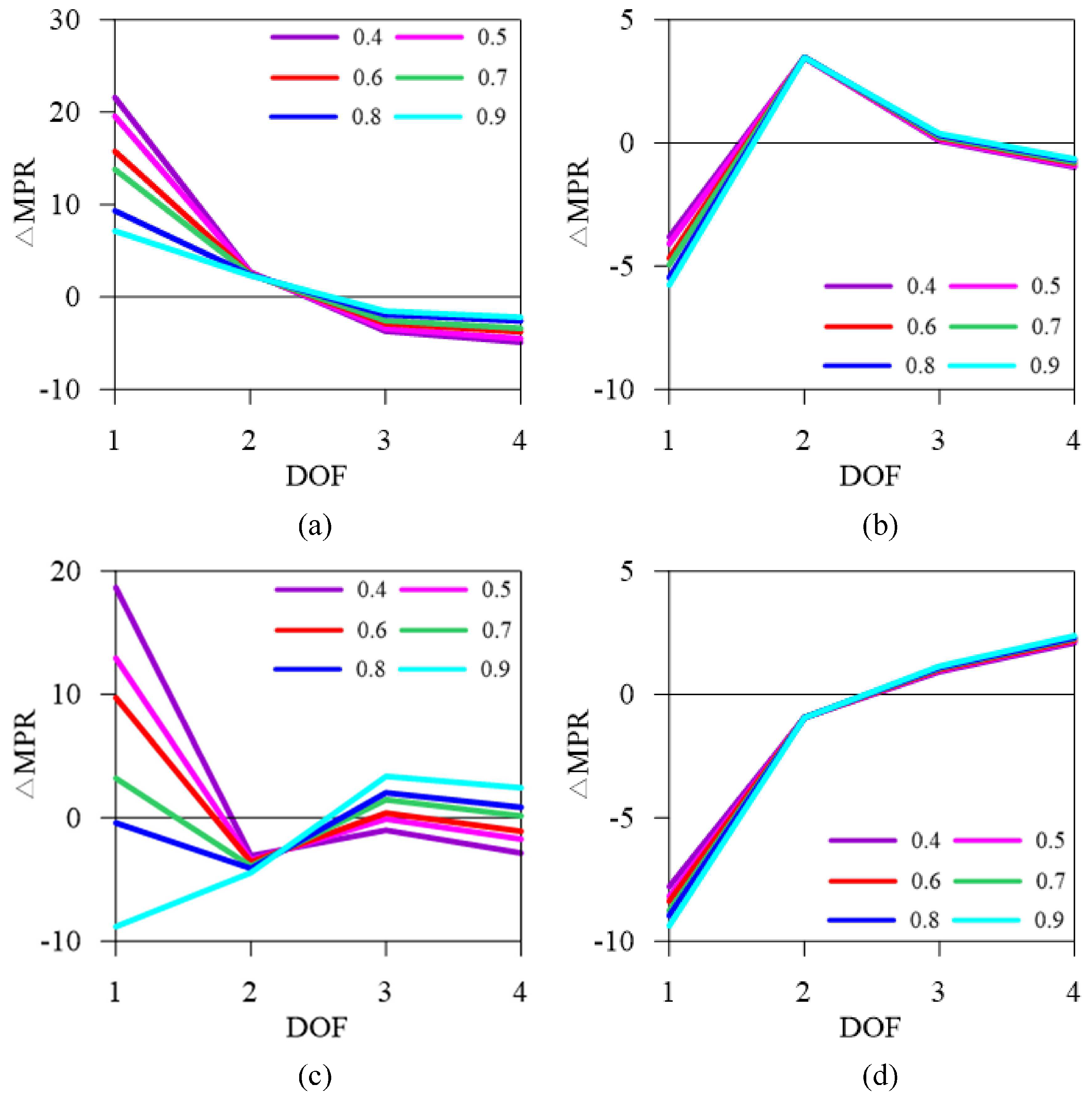
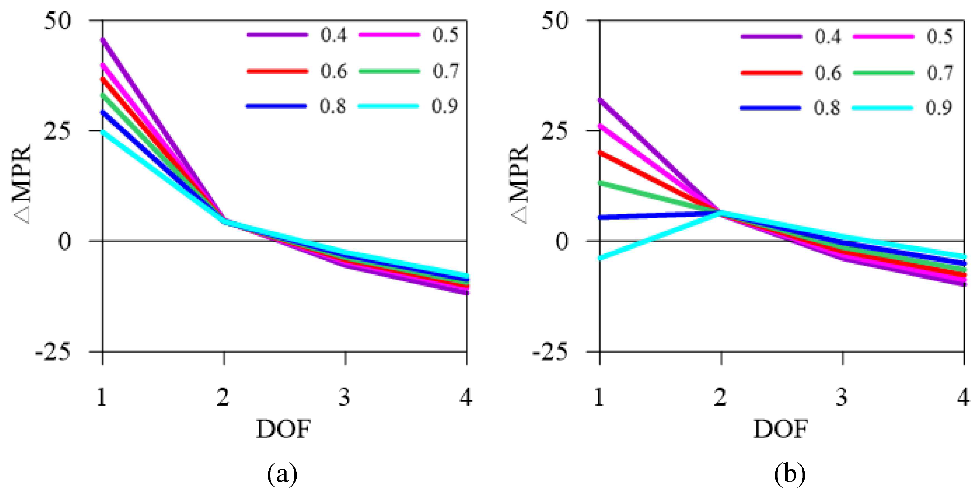
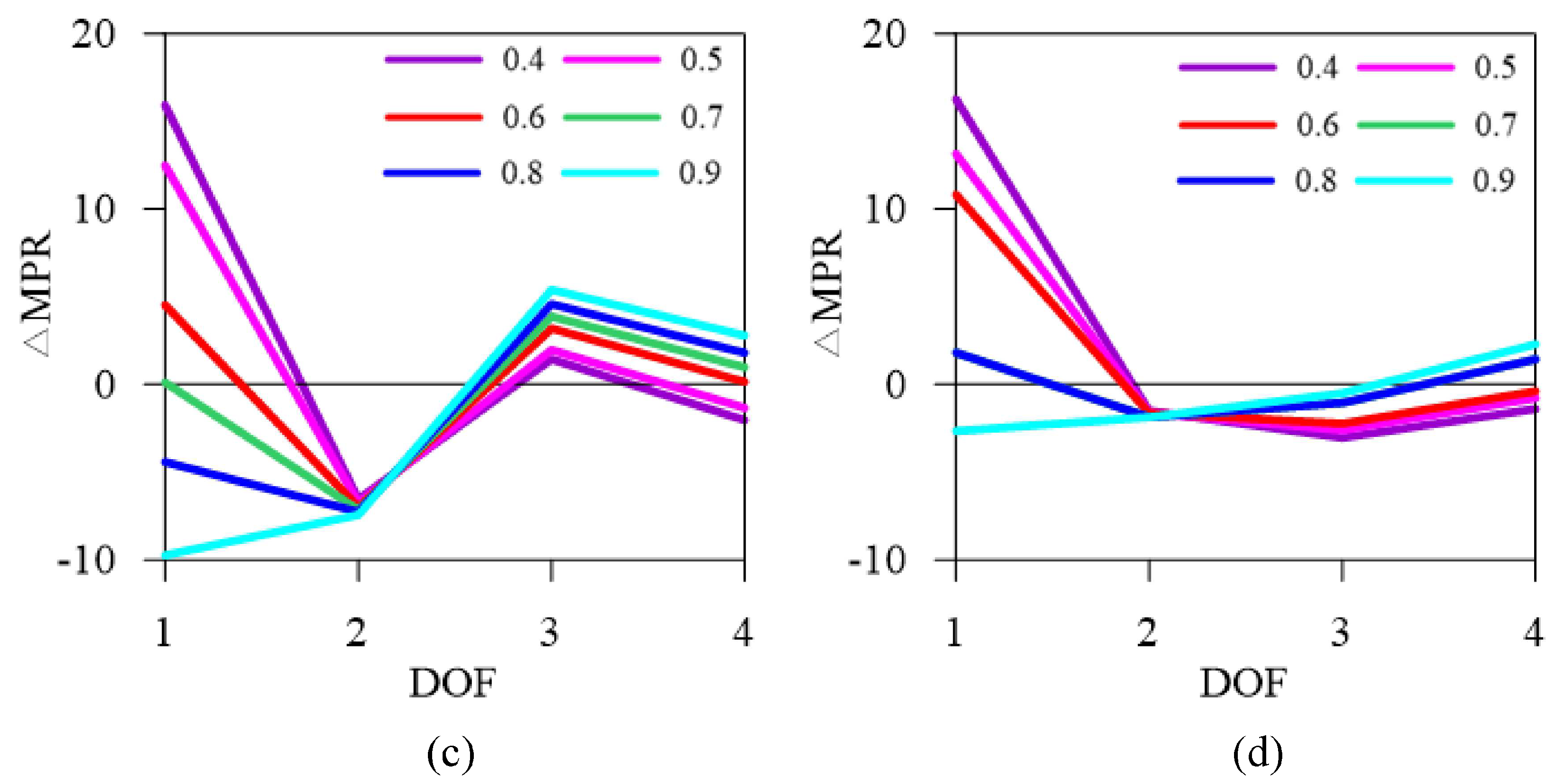
- The proposed filtering procedure called “MAC rejection level” provided more acceptable results for the calculating of MPR values during the damage identification procedure. The MAC rejection level can be taken as 0.9.
Author Contributions
Funding
Data Availability Statement
Conflicts of Interest
References
- Vandiver, J.K. Structural evaluation of fixed offshore platforms. Ph.D. Dissertation, Massachusetts Institute of Technology, Cambridge, MA, USA, 1975. [Google Scholar]
- Adams, R.D.; Cawley, P.; Pye, C.J.; Stone, B.J. A vibration technique for non-destructively assessing the integrity of structures. J. Mech. Eng. Sci. 1978, 20, 93–100. [Google Scholar] [CrossRef]
- Cawley, P.; Adams, R.D. The location of defects in structures from measurements of natural frequencies. J. Strain Anal. Eng. Des. 1979, 14, 49–57. [Google Scholar] [CrossRef]
- Ju, F.D.; Mimovich, M.E. Experimental diagnosis of fracture damage in structures by the modal frequency method. J. Vib. Acoust. 1988, 110, 456–463. [Google Scholar] [CrossRef]
- Lee, Y.-S.; Chung, M.-J. A study on crack detection using eigenfrequency test data. Comput. Struct. 2000, 77, 327–342. [Google Scholar] [CrossRef]
- Rizos, P.; Aspragathos, N.; Dimarogonas, A. Identification of crack location and magnitude in a cantilever beam from the vibration modes. J. Sound Vib. 1990, 138, 381–388. [Google Scholar] [CrossRef]
- Stubbs, N.; Kim, J.T.; Farrar, C.R. Field verification of a nondestructive damage localization and severity estimation algorithm. In Proceedings-SPIE the International Society for Optical Engineering; SPIE International Society for Optical: Bellingham, WA, USA, 1995; p. 210. [Google Scholar]
- Kam, T.-Y.; Lee, T.Y. Detection of cracks in structures using modal test data. Eng. Fract. Mech. 1992, 42, 381–387. [Google Scholar] [CrossRef]
- Wolff, T.; Mark, R. Fault detection in structures from changes in their modal parameters. In Proceedings of the 7th International Modal Analysis Conference, Las Vegas, NV, USA, 30 January–2 February 1989; Volume 1, pp. 87–94. [Google Scholar]
- Yuen, M.M.F. A numerical study of the eigenparameters of a damaged cantilever. J. Sound Vib. 1985, 103, 301–310. [Google Scholar] [CrossRef]
- Pandey, A.K.; Biswas, M.; Samman, M.M. Damage detection from changes in curvature mode shapes. J. Sound Vib. 1991, 145, 321–332. [Google Scholar] [CrossRef]
- Prime, M.B.; Shevitz, D.W. Linear and Nonlinear Methods for Detecting Cracks in Beams; No. LA-UR-95-4008; CONF-960238-10; Los Alamos National Lab. (LANL): Los Alamos, NM, USA, 1995. [Google Scholar]
- Razak, H.A.; Choi, F.C. The effect of corrosion on the natural frequency and modal damping of reinforced concrete beams. Eng. Struct. 2001, 23, 1126–1133. [Google Scholar] [CrossRef]
- Srinivasan, M.G.; Kot, C.A. Effect of Damage on the Modal Parameters of a Cylindrical Shell; No. ANL/CP-74111; CONF-920234-3; Argonne National Lab.: Lemont, IL, USA, 1992. [Google Scholar]
- Salawu, O.S.; Clive, W. Bridge assessment using forced-vibration testing. J. Struct. Eng. 1995, 121, 161–173. [Google Scholar] [CrossRef]
- Nikolakopoulos, P.G.; Katsareas, D.E.; Papadopoulos, C.A. Crack identification in frame structures. Comput. Struct. 1997, 64, 389–406. [Google Scholar] [CrossRef]
- Ovanesova, A.V.; Luis, E.S. Applications of wavelet transforms to damage detection in frame structures. Eng. Struct. 2004, 26, 39–49. [Google Scholar] [CrossRef]
- Curadelli, R.O.; Riera, J.D.; Ambrosini, D.; Amani, M.G. Damage detection by means of structural damping identification. Eng. Struct. 2008, 30, 3497–3504. [Google Scholar] [CrossRef]
- Radzieński, M.; Marek, K.; Magdalena, P. Improvement of damage detection methods based on experimental modal parameters. Mech. Syst. Signal Process. 2011, 25, 2169–2190. [Google Scholar] [CrossRef]
- Altunışık, A.C.; Fatih, Y.O.; Sebahat, K.; Volkan, K. Vibration-based damage detection in beam structures with multiple cracks: Modal curvature vs. modal flexibility methods. Nondestruct. Test. Eval. 2019, 34, 33–53. [Google Scholar] [CrossRef]
- Yu, Y.; Wang, C.; Gu, X.; Li, J. A novel deep learning-based method for damage identification of smart building structures. Struct. Health Monit. 2019, 18, 143–163. [Google Scholar] [CrossRef]
- Khodabandehlou, H.; Gökhan, P.; Fadali, M.S. Vibration-based structural condition assessment using convolution neural networks. Struct. Control. Health Monit. 2019, 26, e2308. [Google Scholar] [CrossRef]
- Pandey, A.K.; Biswas, M. Damage detection in structures using changes in flexibility. J. Sound Vib. 1994, 169, 3–17. [Google Scholar] [CrossRef]
- Liew, K.M.; Quan, W. Application of wavelet theory for crack identification in structures. J. Eng. Mech. 1998, 124, 152–157. [Google Scholar] [CrossRef]
- Mehrjoo, M.; Naser, K.; Moharrami, H.; Bahreininejad, A. Damage detection of truss bridge joints using Artificial Neural Networks. Expert Syst. Appl. 2008, 35, 1122–1131. [Google Scholar] [CrossRef]
- Pawar, P.M.; Reddy, K.V.; Ganguli, R. Damage detection in beams using spatial Fourier analysis and neural networks. J. Intell. Mater. Syst. Struct. 2007, 18, 347–359. [Google Scholar] [CrossRef]
- Huang, M.-S.; Gül, M.; Zhu, H.-P. Vibration-based structural damage identification under varying temperature effects. J. Aerosp. Eng. 2018, 31, 04018014. [Google Scholar] [CrossRef]
- Altunişik, A.C.; Genç, A.F.; Günaydin, M.; Okur, F.Y.; Karahasan, O.Ş. Dynamic response of a historical armory building using the finite element model validated by the ambient vibration test. J. Vib. Control. 2018, 24, 5472–5484. [Google Scholar] [CrossRef]
- Altunisik, A.C.; Karahasan, O.S.; Okur, F.Y.; Kalkan, E.; Ozgan, K. Finite Element Model Updating and Dynamic Analysis of a Restored Historical Timber Mosque Based on Ambient Vibration Tests; ASTM International: West Conshohocken, PA, USA, 2019. [Google Scholar]
- Altunişik, A.C.; Genç, A.F.; Günaydin, M.; Adanur, S.; Yesevi Okur, F. Ambient vibration-based system identification of a medieval masonry bastion for health assessment using nonlinear analyses. Int. J. Nonlinear Sci. Numer. Simul. 2018, 19, 107–124. [Google Scholar] [CrossRef]
- Okur, E.K.; Altunışık, A.C.; Okur, F.Y.; Meral, M.; Yilmaz, Z.; Günaydin, M.; Genç, A.F. Dynamic response of a traditional hımış mansion using updated FE model with operational modal testing. J. Build. Eng. 2021, 43, 103060. [Google Scholar] [CrossRef]
- Luo, J.; Huang, M.; Xiang, C.; Lei, Y. Bayesian damage identification based on autoregressive model and MH-PSO hybrid MCMC sampling method. J. Civ. Struct. Health Monit. 2022, 12, 361–390. [Google Scholar] [CrossRef]
- Soleimani-Babakamali, M.H.; Soleimani-Babakamali, R.; Nasrollahzadeh, K.; Avci, O.; Kiranyaz, S.; Taciroglu, E. Zero-shot transfer learning for structural health monitoring using generative adversarial networks and spectral mapping. Mech. Syst. Signal Process. 2023, 198, 110404. [Google Scholar] [CrossRef]
- Huang, M.; Lei, Y.; Li, X.; Gu, J. Damage identification of bridge structures considering temperature variations-based SVM and MFO. J. Aerosp. Eng. 2021, 34, 04020113. [Google Scholar] [CrossRef]
- Luo, J.; Huang, M.; Xiang, C.; Lei, Y. A Novel Method for Damage Identification Based on Tuning-Free Strategy and Simple Population Metropolis–Hastings Algorithm. Int. J. Struct. Stab. Dyn. 2023, 23, 2350043. [Google Scholar] [CrossRef]
- Malekghaini, N.; Ghahari, F.; Ebrahimian, H.; Bowers, M.; Ahlberg, E.; Taciroglu, E. A Two-Step FE Model Updating Approach for System and Damage Identification of Prestressed Bridge Girders. Buildings 2023, 13, 420. [Google Scholar] [CrossRef]
- Mehboob, S.; Zaman Khan, Q.U.; Ahmad, S. Numerical study for evaluation of a vibration based damage index for effective damage detection. Bull. Pol. Acad. Sci. Tech. Sci. 2020, 68, 1443–1456. [Google Scholar]
- Park, H.S.; Oh, B.K. Damage detection of building structures under ambient excitation through the analysis of the relationship between the modal participation ratio and story stiffness. J. Sound Vib. 2018, 418, 122–143. [Google Scholar] [CrossRef]
- Park, H.S.; Kim, J.; Oh, B.K. Model updating method for damage detection of building structures under ambient excitation using modal participation ratio. Measurement 2019, 133, 251–261. [Google Scholar] [CrossRef]
- Heylen, W.; Stefan, L.; Paul, S. Modal Analysis Theory and Testing; Katholieke Universiteit Leuven: Leuven, Belgium, 1997; Volume 200. [Google Scholar]
- Brincker, R.; Zhang, L.; Andersen, P. Modal identification from ambient responses using frequency domain decomposition. In Proceedings of the 18th International Modal Analysis Conference (IMAC), San Antonio, TX, USA, 7–10 February 2000; Volume 1, pp. 625–630. [Google Scholar]
- Bin Zahid, F.; Ong, Z.C.; Khoo, S.Y. A review of operational modal analysis techniques for in-service modal identification. J. Braz. Soc. Mech. Sci. Eng. 2020, 42, 398. [Google Scholar] [CrossRef]
- Yilmaz, Z. Numerical and Experimental Study of Damage Identification Using Modal Participation Ratio: Detection, Localization and Quantification of Several Damage Scenarios. Master’s Thesis, Karadeniz Technical University, Trabzon, Turkey, 2022. [Google Scholar]
- Oppenheim, A.V.; Buck, J.R.; Schafer, R.W. Discrete-Time Signal Processing; Prentice Hall: Upper Saddle River, NJ, USA, 2001; Volume 2. [Google Scholar]
- Jacobsen, N.-J.; Andersen, P.; Brincker, R. Using enhanced frequency domain decomposition as a robust technique to harmonic excitation in operational modal analysis. In Proceedings of the ISMA2006: International Conference on Noise & Vibration Engineering, Heverlee, Belgium, 18–20 September 2006; Katholieke Universiteit: Leuven, Belgium, 2006. [Google Scholar]
- Batel, M. Operational modal analysis-another way of doing modal testing. Sound Vib. 2002, 36, 22–27. [Google Scholar]
- Rainieri, C.; Fabbrocino, G.; Cosenza, E. Automated Operational Modal Analysis as structural health monitoring tool: Theoretical and applicative aspects. In Key Engineering Materials; Trans Tech Publications Ltd.: Stafa-Zurich, Switzerland, 2007; Volume 347, pp. 479–484. [Google Scholar]
- Yilmaz, Z.; Okur, F.Y.; Gunaydin, M.; Altunişik, A.C. Modal participation ratio in damage identification of building structures: A numerical validation. J. Vib. Control. 2023. [Google Scholar] [CrossRef]
- Computers and Structures Inc. SAP2000. V.21; CSI. PC: Walnut Creek, CA, USA, 2021. [Google Scholar]
- Brüel & Kjær Sound & Vibration Measurement. BK Connect, V. 25.1; B&K. PC: North Denmark, Denmark, 2021. [Google Scholar]
- Brüel & Kjær Sound & Vibration Measurement. PULSE Operational Modal Analysis, V. 7.1; B&K. PC: North Denmark, Denmark, 2021. [Google Scholar]


| Mode | Initial State (Hz) | First Story Damage (Hz) | Second Story Damage (Hz) | Third Story Damage (Hz) | Fourth Story Damage (Hz) | ||||
|---|---|---|---|---|---|---|---|---|---|
| Level #1 | Level #2 | Level #1 | Level #2 | Level #1 | Level #2 | Level #1 | Level #2 | ||
| 1 | 65.248 | 58.878 | 55.776 | 64.057 | 62.666 | 65.616 | 65.048 | 66.723 | 66.839 |
| 2 | 227.732 | 209.526 | 200.864 | 223.367 | 221.288 | 215.512 | 206.9 | 223.968 | 217.989 |
| 3 | 458.989 | 433.068 | 421.78 | 424.473 | 399.393 | 450.838 | 446.798 | 427.197 | 404.473 |
| Frequency Variation (%) | |||||||||
| 1 | 0 | −9.763 | −14.517 | −1.825 | −3.957 | +0.564 | −0.307 | +2.261 | +2.438 |
| 2 | 0 | −7.994 | −11.798 | −1.917 | −2.830 | −5.366 | −9.148 | −1.653 | −4.278 |
| 3 | 0 | −7.514 | −10.927 | −10.667 | −12.984 | −6.538 | −9.196 | −9.029 | −11.877 |
| Mode | Initial State (Hz) | First Story Damage (Hz) | Second Story Damage (Hz) | Third Story Damage (Hz) | Fourth Story Damage (Hz) | ||||
|---|---|---|---|---|---|---|---|---|---|
| Level #1 | Level #2 | Level #1 | Level #2 | Level #1 | Level #2 | Level #1 | Level #2 | ||
| 1 | 67.958 | 61.911 | 58.66 | 60.955 | 59.674 | 66.676 | 64.868 | 68.164 | 68.059 |
| 2 | 231.753 | 212.612 | 200.018 | 224.117 | 224.004 | 216.299 | 208.044 | 224.424 | 210.393 |
| 3 | 459.544 | 425.015 | 409.331 | 410.526 | 377.608 | 429.5 | 417.284 | 418.054 | 385.829 |
| Frequency Variation (%) | |||||||||
| 1 | 0 | −8.808 | −13.682 | −10.305 | −12.190 | −1.886 | −4.547 | +0.303 | +0.149 |
| 2 | 0 | −8.259 | −13.693 | −3.295 | −3.344 | −6.668 | −10.230 | −3.162 | −9.217 |
| 3 | 0 | −7.514 | −10.927 | −10.667 | −17.830 | −6.538 | −9.196 | −9.029 | −16.041 |
| Mode | Initial State (%) | First Story Damage (%) | Second Story Damage (%) | Third Story Damage (%) | Fourth Story Damage (%) | ||||
|---|---|---|---|---|---|---|---|---|---|
| Level #1 | Level #2 | Level #1 | Level #2 | Level #1 | Level #2 | Level #1 | Level #2 | ||
| 1 | 2.943 | 3.536 | 4.088 | 3.699 | 3.715 | 3.295 | 3.464 | 2.938 | 2.897 |
| 2 | 0.972 | 1.034 | 0.991 | 0.954 | 0.936 | 1.022 | 1.022 | 1.003 | 1.103 |
| 3 | 0.505 | 0.533 | 0.542 | 0.571 | 0.625 | 0.551 | 0.554 | 0.507 | 0.579 |
| Damping Ratio Variation (%) | |||||||||
| 1 | 0 | +20.15 | +38.906 | +25.688 | +26.232 | +11.961 | +17.703 | −0.17 | −1.563 |
| 2 | 0 | +6.379 | +1.955 | −1.852 | −3.704 | +5.144 | +5.144 | +3.189 | +13.477 |
| 3 | 0 | +5.545 | +7.327 | +13.069 | +23.762 | +9.109 | +9.703 | +0.396 | +14.653 |
| Structural State | Filtering Parameters | MAC Rejection Values | |||||
|---|---|---|---|---|---|---|---|
| 0.4 | 0.5 | 0.6 | 0.7 | 0.8 | 0.9 | ||
| Undamaged | (Hz) | 32 | 36 | 44 | 52 | 56 | 64 |
| (Hz) | 104 | 100 | 92 | 84 | 80 | 72 | |
| 0.52912 | 0.47026 | 0.35254 | 0.23482 | 0.17596 | 0.05824 | ||
| First Story Damage | (Hz) | 28 | 32 | 40 | 44 | 52 | 56 |
| (Hz) | 92 | 88 | 80 | 76 | 68 | 64 | |
| 0.486 | 0.4214 | 0.29218 | 0.22757 | 0.09835 | 0.03374 | ||
| Second Story Damage | (Hz) | 28 | 32 | 40 | 44 | 52 | 56 |
| (Hz) | 92 | 88 | 80 | 76 | 68 | 64 | |
| 0.50931 | 0.44369 | 0.31244 | 0.24682 | 0.11558 | 0.04995 | ||
| Third Story Damage | (Hz) | 32 | 40 | 44 | 52 | 56 | 64 |
| (Hz) | 104 | 96 | 92 | 84 | 80 | 72 | |
| 0.52007 | 0.40008 | 0.34009 | 0.22011 | 0.16012 | 0.04013 | ||
| Fourth Story Damage | (Hz) | 32 | 40 | 44 | 52 | 56 | 64 |
| (Hz) | 104 | 96 | 92 | 84 | 80 | 72 | |
| 0.52573 | 0.40837 | 0.34969 | 0.23232 | 0.17364 | 0.05628 | ||
| Structural State | Filtering Parameters | MAC Rejection Values | |||||
|---|---|---|---|---|---|---|---|
| 0.4 | 0.5 | 0.6 | 0.7 | 0.8 | 0.9 | ||
| First Story Damage | (Hz) | 32 | 40 | 44 | 48 | 52 | 56 |
| (Hz) | 88 | 80 | 76 | 72 | 68 | 64 | |
| 0.45448 | 0.3181 | 0.24991 | 0.18173 | 0.11354 | 0.04535 | ||
| Second Story Damage | (Hz) | 36 | 40 | 44 | 48 | 52 | 56 |
| (Hz) | 84 | 80 | 76 | 72 | 68 | 64 | |
| 0.39672 | 0.32969 | 0.26266 | 0.19563 | 0.1286 | 0.06157 | ||
| Third Story Damage | (Hz) | 36 | 40 | 48 | 52 | 56 | 60 |
| (Hz) | 92 | 88 | 80 | 76 | 72 | 68 | |
| 0.41826 | 0.3566 | 0.23327 | 0.17161 | 0.10995 | 0.04828 | ||
| Fourth Story Damage | (Hz) | 44 | 48 | 52 | 60 | 60 | 64 |
| (Hz) | 92 | 88 | 84 | 76 | 76 | 72 | |
| 0.35177 | 0.293 | 0.23422 | 0.11668 | 0.11668 | 0.05791 | ||
Disclaimer/Publisher’s Note: The statements, opinions and data contained in all publications are solely those of the individual author(s) and contributor(s) and not of MDPI and/or the editor(s). MDPI and/or the editor(s) disclaim responsibility for any injury to people or property resulting from any ideas, methods, instructions or products referred to in the content. |
© 2023 by the authors. Licensee MDPI, Basel, Switzerland. This article is an open access article distributed under the terms and conditions of the Creative Commons Attribution (CC BY) license (https://creativecommons.org/licenses/by/4.0/).
Share and Cite
Yilmaz, Z.; Okur, F.Y.; Günaydin, M.; Altunişik, A.C. Enhanced Modal Participation Ratio-Based Structural Damage Identification: A New Filtering Approach Using Modal Assurance Criteria. Buildings 2023, 13, 2467. https://doi.org/10.3390/buildings13102467
Yilmaz Z, Okur FY, Günaydin M, Altunişik AC. Enhanced Modal Participation Ratio-Based Structural Damage Identification: A New Filtering Approach Using Modal Assurance Criteria. Buildings. 2023; 13(10):2467. https://doi.org/10.3390/buildings13102467
Chicago/Turabian StyleYilmaz, Zafer, Fatih Yesevi Okur, Murat Günaydin, and Ahmet Can Altunişik. 2023. "Enhanced Modal Participation Ratio-Based Structural Damage Identification: A New Filtering Approach Using Modal Assurance Criteria" Buildings 13, no. 10: 2467. https://doi.org/10.3390/buildings13102467
APA StyleYilmaz, Z., Okur, F. Y., Günaydin, M., & Altunişik, A. C. (2023). Enhanced Modal Participation Ratio-Based Structural Damage Identification: A New Filtering Approach Using Modal Assurance Criteria. Buildings, 13(10), 2467. https://doi.org/10.3390/buildings13102467