
Building Performance under Untypical Weather Conditions: A 40-Year Study of Hong Kong

1
School of Civil Engineering, Guangzhou University, Guangzhou 510006, China
2
School of Architecture and Urban Planning, Guangzhou University, Guangzhou 510006, China
*
Authors to whom correspondence should be addressed.
Buildings 2023, 13(10), 2587; https://doi.org/10.3390/buildings13102587
Submission received: 8 September 2023
/
Revised: 10 October 2023
/
Accepted: 10 October 2023
/
Published: 13 October 2023
(This article belongs to the Special Issue Advances in Building Performance Simulation and Building Energy Consumption Analysis)
Abstract
:As a common engineering practice, the buildings are usually evaluated under the Typical Meteorological Year (TMY), which represents the common weather situation. The warm and cool conditions, however, can affect the building performance considerably, yet building performances under such conditions cannot fully be given by the conventional TMY. This paper gives approaches to constructing the weather data that represents several warm and cool conditions and compares their differences by studying the cumulative cooling demands of a typical building in a hot and humid climate. Apart from the Extreme Weather Year (EWY), the Near-Extreme Weather Year (NEWY) and Common warm/cool Years (CY) data are proposed according to the occurrence distributions of the weather over the long term. It was found that the cooling demands of NEWY and EWY differ by 4.8% from the cooling needs of TMY. The difference between the cooling demands of NEWY and CY for most calendar months can be 20% and 15%, respectively. For the hot months, the cooling demands under NEWY and CY take 7.4–11.6% and 2.3–5.6% differences from those under TMY. The uncertainties of building performance due to the ever-changing weather conditions can be essential to the robustness of building performance evaluations.
1. Introduction
Buildings are consuming around 40% of society’s total energy [1,2] for the comfort and well-being of their occupants in the ever-changing outdoor environment. Academia focuses on buildings’ energy and thermal performance [3], operation strategies [4], and materials [5] in specific climatic conditions. With advancing computer technology, experts often use simulation tools [6] for building performance studies. Beyond the building’s design, the outdoor climate significantly influences simulation outcomes [7,8]. Due to the comprehensive influence of astronomical, geographical, and human activity factors, outdoor climate conditions can vary year-by-year [9], imposing uncertainties in evaluating the expected energy, indoor environment quality, and the performances of energy-saving strategies [7] and renewable energy productions [10,11] by simulations. Previously, weather data were chosen to represent typical long-term conditions. The approach saves computation costs in evaluating the building performance using the so-called “most representative” climate over a long period of 30 years or so [12]. This representative weather is either determined by selecting one whole year as the ASHRAE Test Reference Year (TRY) [13] or by picking 12 months one by one and combining them as Hall’s Typical Meteorological Year (TMY) [14], the Weather Year for Energy Calculations (WYEC) [15], and the Chinese Standard Weather Data (CSWD) [16]. However, a building’s performance in “typical” weather might not reflect its behavior in prolonged warm or cold scenarios [17]. With an increasing focus on the safety of thermal environments [18], it is becoming increasingly important to study building energy and thermal performances under various weather conditions that can be different from normal conditions.
Numerous studies have sought to identify data representing warm and cool conditions over extended periods. Warm climate conditions, for example, are sometimes identified by ranking the average or peak values of the summer dry-bulb temperature [19] or cooling degree days (or hours) over a long-term period using the measured or generated weather data. The Design Summer Year (DSR) [20], near-extreme Design Reference Year (DRY) [21], and Hot Summer Year (HSY) [22] datasets are determined under this framework. Similarly, the Summer Reference Year (SRY) [23] adopts the highest 5% recordings of the weather variables only for ranking the years of interest from cold to warm; the features and regulations of the variable values representing warm and typical conditions are studied further. Later, the typical hot year (THY) [24] is developed by multiple aggregative or peak-value indices, such as the total or maximum degree hours (or days) when the (daily maximum) temperature is above a threshold and the maximum length of such events.
The cumulative or peak-value indices may be reasonable to identify the untypical cases with higher/lower-than-usual temperatures. However, approaches identifying the weather conditions by an average or cumulative value can be less comprehensive than those by the occurrence frequency distributions of the weather variables (such as TMY), especially when the energy of a whole month or year instead of a few extreme days is considered. Yet, the previous occurrence-based study was limited to adjusting the weight of the extreme values among various climatic indices [25], which can be more applicable to the adaptive adjustments of the TMY for various purposes than identifying the various climatic conditions. Recently, the occurrence-based approach has been used to identify extreme weather by dry-bulb temperature from both historical weather records and future expectations under the changing climate [26]. The importance of considering the extreme years is illustrated later [27]. The approach was extended for humidity-related studies, with relevant variables included [28]. Unlike typical years, this extreme year approach selects the months that take the greatest differences from the long-term trend by the occurrence distribution of the climatic variables. Although the extreme years can scale the potential range of the building performances without excessive simulations over several decades, the occurrence probability of the extreme cases that are far from the weather over the long term is not considered. The extreme weather conditions, if turned out to be outliers, would have few implications for the building performance studies that attempt either “representative” warm or cool conditions for energy savings or relatively severe conditions for the system designs. Extreme conditions are usually “not-guaranteed” [29] in the thermal designs of buildings. It can thus be essential to identify the warm and cool conditions according to their occurrence instead of the peak and bottom values. In this case, the uncertainties of the current typical and extreme weather conditions and their impacts on building performance should be studied.
Apart from the uncertainties of the various possible weather conditions in studying the building performances, another uncertain issue in identifying the weather conditions is the comprehensiveness of the accessible weather variables in depicting the weather variations. Due to the difficulties in acquiring the solar radiation data in both the historical measurements and the simulation-based future expectations [30], several studies on identifying the (near-)extreme weather conditions relied on the recorded or simulated dry-bulb temperature only [26,31]. This brings benefits in saving the cost of data measurements [32], yet uncertainties in missing the impact of a few weather data that affect the building performance. Considering the different focuses in identifying the common and extreme weather conditions, it may be sufficient to depict the extreme weather conditions for building performance studies using fewer variables than TMY, while the uncertainties should be quantified.
This paper intends to evaluate the uncertainties of the building performance studies under various weather conditions and test the possibility of identifying the “representative” warm and cool weather conditions for different purposes and using different available climatic variables. The differences between the yearly and long-term weather data for each calendar month are quantified by their cumulative frequency of occurrences, like the TMY and Nik’s [26,27,28] framework. The occurrence instead of the max or min values of the differences determines the warm and cool weather conditions.
In this paper, the uncertainty of the weather condition and its consequences on building performance are exemplified by the well-recorded hourly weather data over the long term and the well-developed representative building model of Hong Kong. The results can be representative of places with similar climates and building types, such as the cities in the Pearl Rivel Delta and subtropical regions. The representativeness is because of the similar climate, cultural background, occupant operation schedules, and urban densities of the cities in the region. The following sections are arranged as follows: Section 2 gives the methodology for quantifying the differences between the yearly and long-term weather conditions according to the distributions of their values over the corresponding periods. Section 3 analyzes the distributions of these climatic differences for all calendar months over decades using the data from Hong Kong; the various untypical weather conditions for different engineering purposes and the cumulative cooling demands under these scenarios are determined. Implications for the building performance studies are discussed.
2. Methodology
2.1. Differences between Yearly and Long-Term Weather Conditions
This study uses weather data from long-term ground measurements spanning several decades to represent both typical and extreme weather conditions. The weather data is analyzed monthly based on various rules and then aggregated into yearly data for specific objectives. For each month, the cumulative distribution functions (CDF) of various variables are determined by Equation (1) using either the data of the long-term over decades or the data of each year.
For the period under consideration, means the occurrence rate of a weather variable that is lower than its value , and the index ranges from 1 to the number of the non-repeating values in the period n. In this case, for each of the 12 calendar months, a series of can be calculated every year, and the average of its differences from the CDF using all data of the same month over decades is known as the Finkelstein-Schafer statistics [33], which can be written as Equation (2a). While seeking the (near-)extreme years, however, the gaps between the yearly and overall CDF values are calculated as the average of the differences without taking absolute values instead, as given by Equation (2b). In this case, the CDF values of the warm and cold years can usually be, respectively, lower and higher than the CDF over the long term, indicating the differences in the climatic conditions.
The weather conditions can be affected by more than one weather variable, and their differences from the long-term climatic conditions (shown by the index) are not necessarily the same. In this case, the of multiple climatic variables is studied together as Equation (3) using their corresponding weights . The scale of indicates the relative importance of the variable under consideration. Conventionally, variables such as daily average dry-bulb temperature and daily total solar radiation are given high weights for their importance in influencing building performances, though the radiation is not readily accessible in many places around the world. The quantifies the similarities between the yearly and long-term weather, considering the occurrence and distribution of multiple variables.
2.2. Identifying the Weather Conditions
For each of the 12 calendar months, the current works identify the typical and extreme weather as the years taking the minimum and a high WS over a long period, respectively. Without studying the occurrence of the WS values over the long-term period, however, the effectiveness of the extreme months in representing warm and cold conditions remains unclear. In this study, we set various occurrence-based rules to depict various weather scenarios over the long term, which include:
- Extreme weather years (EWY) that take the highest positive or negative WS values.
- Near-extreme weather years (N-EWY) that take the highest positive or negative WS values, excluding the outliers.
- Common warm and cold years (CY) with the absolute of their positive or negative WS values that are (or closest to) the absolute WS values over the period under consideration.
- TMY takes the least absolute WST as a reference for various weather conditions.
Here, the CY stands for the warm and cold weather conditions that have the greatest occurrence probability if the absolute follows the normal distribution over the long-term period. The N-EWY excludes the extreme weather that drifts far away from the rest of the period and takes a low occurrence chance. The outliers are determined by two criteria based on either the interquartile range or the Standard Score (sometimes called the Z-score). The interquartile range method determines the upper and lower thresholds of the WS values using Equations (4a) and (4b). Here, and are, respectively, the 1st and 3rd quartiles of the 42-year values of each calendar month. Meanwhile, the values are converted to the Z-score by Equation (5) according to the average and standard deviation of the WS values of the same calendar month for each of the 42 years. In this study, the coefficient takes one, and the limits of the Z-score take 2 and −2. The two criteria are used in case the values over the 42 years of each calendar month are not showing normal distribution features, though the criteria are equivalent to normal distributions. Such settings remove around 4% of the data if they are normally distributed, suggesting that one warm year and one cold year can be removed every 50 years.
To quantify the WS and WST in weather data development, we consider various climatic variables, including horizontal global radiation (GSR), dry-bulb temperature (DBT), dew point temperature (DPT), relative humidity (RHM), wind direction and speed (WSP), and cloud coverage. Yet not all variables are available for any place in the world in either historical records or future estimations. Thus, in this research, we tested the uncertainties and validities of identifying the weather conditions by all or a part of the variables among DBT, DPT, GSR, and WSP, according to their performances in studying the potential cooling demands. The weights of the variables for identifying the typical, warm, and cool weather scenarios are listed in Table 1. The GSR-only and DBT-only tests evaluate the validity of the extreme conditions selected by GSR and DBT only, which either have good accessibility or are important to the diurnal cooling load of the buildings. In other words, the performances and opportunities of identifying warm and cool weather conditions by DBT and/or GSR are tested.
The data were acquired from ground meteorological measurements by the Hong Kong Observatory, a governmental weather agency. The site of the weather observatory was on a hill in the downtown of Hong Kong (King’s Park) that was relatively free of surrounding obstructions. Only the global horizontal solar radiation was measured before 2008, and the direct and diffuse components of the solar radiation were estimated by models as the process of the current TMY. In August 2008, an observation site was established in the suburb (Kau Sai Chau) of the administrative region that takes measurements of global, direct, and diffuse solar radiation. The 42-year data from 1979 to 2020 is used.
2.3. The Typical Building for Weather Data Testing
The importance of various weather conditions, including the typical, (near-)extreme, and common warm/cool ones, is further depicted by the cooling demands of a building. Though Hong Kong is well-known for its compact urban development, it can be difficult to determine a certain urban layout for the building under consideration. In this case, the impacts of various design weather conditions are evaluated by a stand-alone 27-level building (gross area = 20,000 m2) that is representative of the local social and technical norms, as shown in Figure 1. The light-colored squares on the envelope represent the windows of the building. The typical building is determined by a local design guide from Hong Kong SAR [34] and has been used in several previous building meteorological studies [35,36,37]. Without obstruction being considered, the potential impact of the uncertainty of solar radiation on building performance can somehow be overestimated. However, it is reminded that the uncertainties of the weather conditions are depicted by dry-bulb and dew point temperatures, which show similar fluctuation trends to the radiation.
There are air-conditioned commercial spaces on floors 1 to 3, car parts on floors 4 to 5 that are sized at 40 × 40 m2, and air-conditioned offices on rest floors that are sized at 20 × 30 m2. The internal load densities and fresh air amounts for various areas are specified in Table 2, and their operation schedules can be found according to the design guidelines of the local government [38]. The infiltration rates are set at 1.4, considering the results of the opening-window activities of occupants in corridors. The 25 °C cooling setpoint refers to a previous study of the same place [39]. Free cooling is not used because of the considerably high outdoor humidity. Table 3 gives the thermal properties of the building envelope. The 6 mm clear glass is used, according to the design guideline, because of the high solar altitude angle at the summer noon. The hourly building cooling demands are calculated by the well-acknowledged EnergyPlus simulation software (version 9.0.1) [40]. Since this study focuses on the comparison of the different weather conditions, an ideal air-conditioning system was used for simplicity, in which case the system always satisfies the cooling demand perfectly. No surrounding obstructions nor the urban heat island were considered as well.
3. Results
3.1. Differences between Yearly and Long-Term Weather Conditions
Figure 2 presents the distributions of WST values, determined using all climatic variables listed in Table 1, in line with the conventional approach for TMY. For each calendar month, the case with the least WST (around 0.05) is “assembled” for the TMY. It was found that none of the lowest WST cases were regarded as outliers. However, for most months except September, the highest WST values were identified as outliers. The recurring outliers and the WST range highlight significant risks in estimating building performance using only TMY without considering atypical conditions or WS distributions. On the other hand, the boxes of all calendar months, as the ranges of WST between the 1st and the 3rd quartile, are relatively compact compared to their corresponding whiskers. The compact ranges suggest that a number of years can take a moderate difference of WST values around 0.1 from the long term, and such a difference is higher than the lowest value of 0.05 of the conventional TMY. In this case, the warm or cold years with a WS close to the corresponding medium value may represent the “common” warm or cold cases that have high occurrence probabilities and notable differences from the weather feature over the long term.
Figure 3 displays the WS values for each month, as determined by Equation (3b), without accounting for the absolute differences. The mid-values of WS are around zero, indicating the occurrence probabilities of the warm and cold years are similar for all calendar months. The results in Figure 3 without absolute values are useful in identifying the year(s) with (near-)extreme weather conditions whose CDFs are usually shifted to a single side of the long-term CDF curve. A part of the positive and negative δ cancels out for cases with overlapping yearly and overall CDF curves, giving a low WS value that indicates the monthly cooling or heating demands are similar to the long-term average. According to Figure 3, the outliers are identified by the interquartile ranges in Jan, Mar, May to Sep, Nov, and Dec for their considerable difference from the median values. In addition, additional outliers are identified by the Z-score instead of the interquartile method, especially for Feb, considering the extensive range of its WS values. There are consistencies among the outliers in Figure 2 and Figure 3, while their differences are mainly because of the changes in the upper and lower whiskers and the canceling out of the differences with different signs while comparing the yearly and long-term CDF.
Figure 4a and Figure 4b give the WS that is quantified by the DBT only and GSR only, respectively. The WS in Figure 4c is determined by GSR and DBT without other variables. Comparing Figure 3 and Figure 4 reveals that WS derived from multiple variables has shorter whiskers and potentially fewer uncertainties than when determined by just one variable, notably the DBT. Although consistent trends in the monthly WS distributions are found in Figure 3 and Figure 4a, the distributions of the latter are more scattered than the former. This difference is probably because of the various climatic variables of a single year that cause different up- or down-shifting disparities in the long term, corresponding to different cooling or warming effects of the environment. A part of the outliers in the Mar of the “All” case was not recognized by DBT because of the extensive WS distributions in Figure 4a. Likewise, the WS determined by GSR only in Figure 4b were more scattered than that determined by all climatic variables (shown in Figure 3), and their outliers are thus different, especially for Mar and Jun. On the other hand, the WS distributions shown in Figure 3 and Figure 4c are similar, and this is probably due to the high weights of GSR and DBT in the “All” case. The comparison between Figure 3 and Figure 4 suggests the uncertainties of identifying the (near-)extreme weather by GSR and/or DBT, and this should be studied further by their impacts on the representative local buildings.
Though the warm and cool conditions can be identified by Figure 3 and Figure 4 for each calendar month, the expected temporal length of the untypical weather and their influences on the buildings over a period longer than a month remain unclear. The auto-correlation coefficients of the monthly WS are thus studied and plotted in Figure 5. Here, for each year, the monthly WS from Jan to Dec is compared to the series with 1 (i.e., Feb to Mon) to 6 months delayed, and the process repeats for all 42 years under consideration. An ρ value higher than 0 suggests that the warm or cool trend of a month is consistent with the trends several months later. In other words, the auto-correlation tests whether the warm or cool feature of a single month tends to be kept 1 to 6 months later. The values of ρ, as shown in Figure 5, take a higher probability to be positive than negative when the gap between the months of interest is no greater than one, and the ρ reduces when the gap increases from 1 to 4 months. For cases with a 1-month gap, according to the occurrence distribution, the peak occurrence of ρ is found around 0, indicating the two neighboring months have low probabilities of being negatively correlated. For cases with gaps greater than 2 months, on the other hand, a considerable occurrence can be found for ρ < 0. The results suggest the warming or cooling tendencies usually last for no more than two months, and there is some kind of “balance” between the warm and cool occurrences over a short period.
3.2. Building Cooling Demands in Various Weather Conditions
Figure 6a demonstrates the cooling demands of the typical local building that are determined by the typical, warm, and cool weather conditions using “All” climatic variables (All-row in Table 1) as the conventional TMY. This includes the warm and cool conditions depicted by the EWY, NEWY, and CY weather datasets; the cooling demands under these weather conditions are compared to TMY, and their absolute differences are plotted in Figure 6b,c. The cooling demands of the TMY and its occurrence under weather conditions over the past 42 years are plotted in Figure 6a for comparison and reference. It is not surprising that the cooling demands being estimated by TMY lie in the center of the potential range under all possible weather conditions for all calendar months. The cooling demands estimated by the EWY, on the other hand, lie at the upper and lower ends for most calendar months. For a few months like Nov and Apr, however, the cooling demands of EWY may not exactly be the highest or lowest over the long period under consideration since the building operates 1/3 of the day.
The EWY, NEWY, and CY represent the weather conditions at different extreme levels and occurrence probabilities, which determine various building cooling demands for different engineering purposes. For most months, the average differences between the monthly cooling demands of EWY and TMY are around 10 MJ/m2 for warm and cool cases, according to Figure 6b,c. The NEWY, on the other hand, avoids the outlier cooling demands, especially for May, Jun, July, and Sep months, which usually correspond to relatively high needs for cooling throughout the year. For the warm case, the cooling demands of NEWY and EWY can make a difference of around 3.5 MJ/m2/month for the summer and winter periods from May to Jul and Jan to Feb; the difference is around 2 MJ/m2/month for the entire year. The difference of 3.5 MJ/m2/month from Mar to Jul accounts for up to 4.8% of the cooling demands under TMY. The cooling demands under the CY, in addition, take a 6 MJ/m2/month difference on average from the cooling demands under the TMY. Interestingly, as shown in Figure 6a, the cooling demand of the warm NEWY and CY are close to the TMY from Dec to Feb, which is a result of their right-skewed occurrence distributions of the cooling demand over the 42 years. The results show NEWY and CY can be important to supplement the TMY-based building performance studies, especially for those requiring consideration of weather uncertainties.
Figure 7 and Figure 8 give the building cooling demands of the NEWY, EWY, and CY that are identified by DBT and/or GSR. Figure 7a and Figure 8a show that it is not proper to identify the NEWY warm nor the cool conditions using GSR only, since the cooling demand estimations are not stable and are similar to those of TMY, especially for winter periods. In this case, the CY determined by GSR only is not considered as well. To evaluate the validity of the untypical weather conditions being identified by a part of climatic variables, their corresponding building cooling demands are compared to the weather datasets being identified by “All” variables. Such cooling demand differences (i.e., weather data identified by DBT or DBT&GSR–weather data identified by “All” variables) for the (warm or cool) NEWY and CY weather conditions are given in subplots (b) and (c) of Figure 7 and Figure 8, respectively.
The untypical years identified by DBT only or DBT&GSR (T&R), on the other hand, give relatively low differences from the “All”-variable cases, which are less than ±3 MW/m2 and ±4 MW/m2 for most warm cases (Figure 7) and cool years (Figure 8), respectively. The differences between NEWY given by Figure 7b and Figure 8b are somehow lower than the difference between CY given by Figure 7c and Figure 8c, suggesting that NEWY can be identified more “stably” than CY when comprehensive weather observations are not available. Meanwhile, the differences between the R&T-based climatic identifications are slightly lower than the DBT-based ones for most cases, especially for the cool NEWY and CY in Figure 8b,c, yet the differences between the DBT and T&R are comparable for the warm NEWY, according to Figure 7b. In this case, it can be preferable to identify the CY by both DBT and GSR measurements, yet the NEWY identified by DBT without GSR can be acceptable for identifying the warmer-than-TMY conditions, especially the NEWY as shown in Figure 7b.
The relative differences in estimating the cooling demands under the “untypical” weather and TMY for the 12 calendar months are given in Figure 9, which shows the similarities of common or near-extreme weather conditions in various months and the uncertainties of the TMY under various warm or cool weather conditions. If long-term weather data is unavailable, the cooling demands for various CY and NEWY conditions can be estimated using the relative difference from the easily accessible TMY. According to the median of the distribution, the cooling needs of the NEWY take differences of around 20% from the TMY for most warm and cool cases, while such a difference is higher than 10% for the common years. As for the ranges of the box and whiskers in Figure 9, the cooling demands of NEWY in various months can usually take a wider range than that of CY. The box ranges of CY are around 15% for most cases, while this range can be higher than 20% for many NEWY cases, especially for the cooler-than-TMY cases. The results suggest the monthly cooling needs under CY may be estimated by the routine TMY data with lower uncertainties than the NEWY. Interestingly, the cooling demand differences tend to cluster in a lower range for the warm conditions than the cool cases for the place under study. Meanwhile, the NEWY and CY identified by DBT usually take slightly lower ranges compared to those determined by DBT+GSR (R&T), suggesting the good performance of DBY in identifying weather conditions when the “sophisticated” variables are not available.
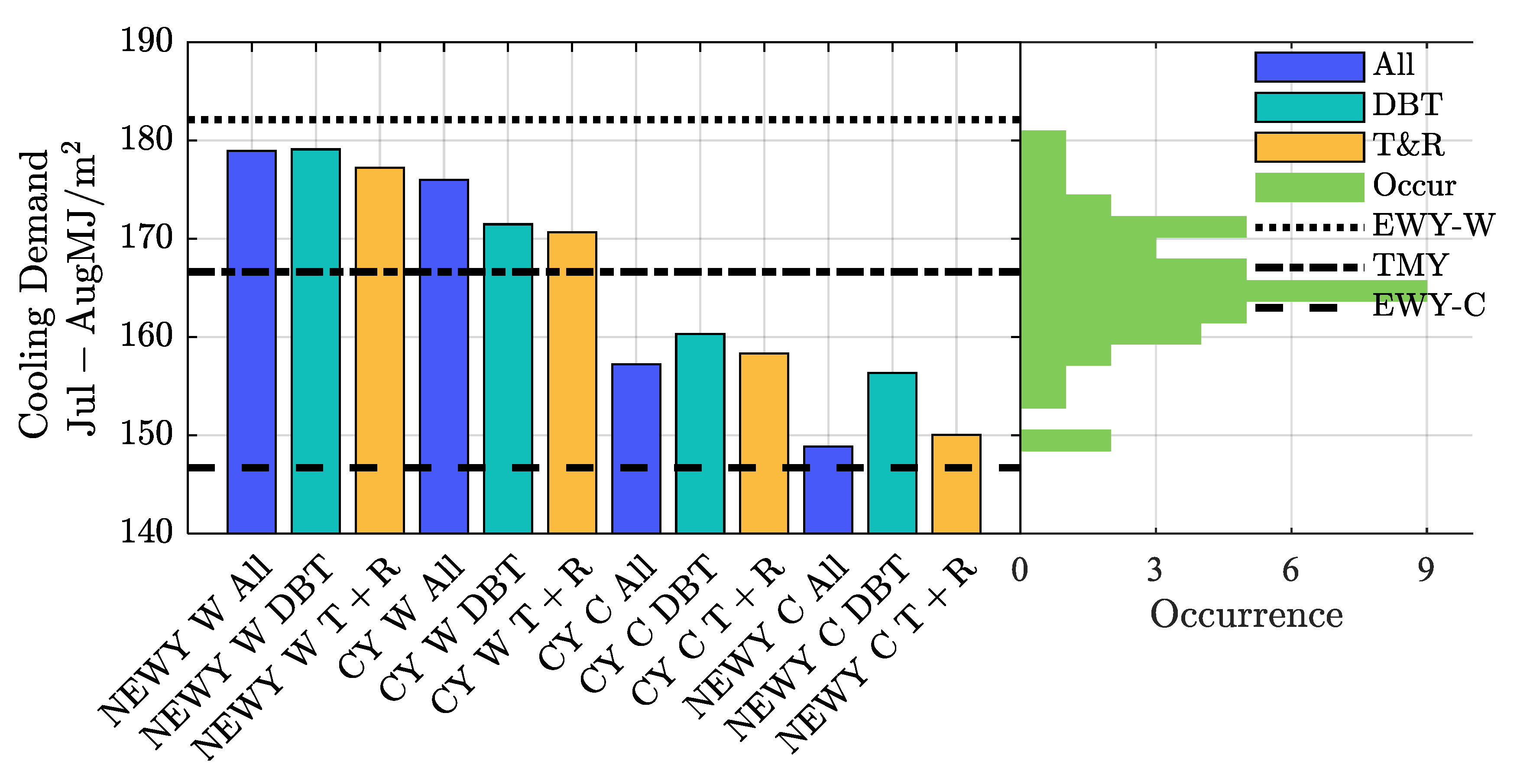
The differences in the cooling demands from Jul to Aug under different weather conditions are specified in detail as shown in Figure 10. The cooling needs of the two successive summer months are compared as the warm or cool conditions extend for ≤two months, as shown in Figure 5. Jul and Aug are selected for the highest building cooling needs in these months, and the results suggest the potential “cumulative” impact of the warm or cool weather on the building energy. The up-shifting cooling demands under TMY in Figure 10 were due to the distribution that slightly shifted to the high-value side. According to Figure 10, the difference in the building cooling needs between the EWY and NEWY can be 3.2 MJ/m2 for the warm case, which accounts for around 2% of the cooling needs under TMY. The difference in the cooling demands for the NEWY and TMY cases, meanwhile, can be 12.3 MJ/m2 MJ for the most warm datasets and 17.7 MJ/m2 for the cool datasets, accounting for 7.4% and 10.6% of the cooling needs under the TMY. For common untypical cases, such differences can be around 3.9 to 9.4 MJ/m2 (2.3% to 5.6%) for warm CYs and 6.3 to 9.4 MJ/m2 (3.8% to 5.6%) for cool CYs. The ranges show the notable uncertainties of the cumulative building cooling demand estimations by TMY only.
4. Conclusions
This paper studies the uncertainties of building performance evaluations using fully typical or extreme weather conditions and proposes methods for determining the weather data of the warm and cool scenarios according to the occurrence of various weather conditions over four decades. Apart from the conventional Typical Meteorological Year and the Extreme Weather Year (EWY), our research proposes the datasets of the Near Extreme Weather Year (NEWY) and Common Year (CY) by the 42-year ground measurement of Hong Kong. The NEWY excludes the outlying meteorological months of extreme and “not-guaranteed” weather conditions, and the CY represents the “representative” untypical weather conditions that are different from the TMY.
According to the typical building for the local society, accepting or declining the outlying weather conditions can give a 3.5 MJ/m2/month difference in the cooling demands, accounting for 4.8% of the cooling demand under the TMY. In cases where the “sophisticated” meteorological variables are not accessible, it can be acceptable to identify the warm and cool conditions using the dry-bulb temperature with or without global radiation. Meanwhile, it is found that the relative cooling demand differences between the NEWY and CY and those of the TMY are roughly 20% and 15% for most cases, respectively. Though such differences vary month by month, their ranges for CY can be lower than those for NEWY. The warm and cool cases usually extend for less than two successive months, and the cumulative cooling demands of the warm or cool cases over the hottest two months (Jul and Aug) account for 7.4–11.6% and 2.3–5.6% of the TMY for the NEWY and CY, respectively. Greater differences can be found in the relatively cool months.
According to the results, the buildings are likely to bear different weather conditions that raise a wide range of energy demands, though TMY, in principle, depicts the most probable case. The ranges of cooling demands show the weakness and risks of evaluating the performance, energy demand, environment, and energy safety of buildings and even the entire society using a single set of weather data. The probability of the various weather conditions, with various differences from the mostly probable TMY, is well given for robust energy and environmental studies for buildings and even society.
Major limitations of the current research include the insufficiencies of the types of weather conditions, buildings, and city environments. In the future, it is expected to evaluate the robustness of the current results by adopting various types of building functionality, surrounding obstructions, and places with different weather conditions. The influences of the weather uncertainty on the building performance can be different when the loads, solar accessibility, and weather uncertainties are changed by the building types, urban densities, and climates. These issues are worth investigating in future studies.
Author Contributions
Conceptualization, S.L. and Y.Z.; methodology, S.L. and Y.H.; software, Z.P.; validation, J.C., Y.Z. and Y.H.; investigation, Z.P. and J.C.; resources, Y.H.; data curation, Y.Z.; writing—original draft preparation, S.L.; writing—review and editing, S.L. and Y.H.; visualization, Z.P. and J.C.; supervision, Y.Z. and Y.H.; funding acquisition, Y.Z. All authors have read and agreed to the published version of the manuscript.
Funding
This research was funded by the National Natural Science Foundation of China, grant number 52308016; the Guangdong Basic and Applied Basic Research Foundation, grant number 2023A1515011364; and the Science and Technology Program of Guangzhou University, grant number PT252022006.
Data Availability Statement
Data is available on request due to privacy restrictions.
Conflicts of Interest
The authors declare no conflict of interest.
References
- Zhu, H.-C.; Ren, C.; Cao, S.-J. Fast prediction for multi-parameters (concentration, temperature and humidity) of indoor environment towards the online control of HVAC system. Build. Simul. 2021, 14, 649–665. [Google Scholar] [CrossRef]
- Yuan, X.; Pan, Y.; Yang, J.; Wang, W.; Huang, Z. Study on the application of reinforcement learning in the operation optimization of HVAC system. Build. Simul. 2021, 14, 75–87. [Google Scholar] [CrossRef]
- Wang, R.; Lu, S.; Zhai, X.; Feng, W. The energy performance and passive survivability of high thermal insulation buildings in future climate scenarios. Build. Simul. 2022, 15, 1209–1225. [Google Scholar] [CrossRef]
- Kong, X.; Chang, Y.; Li, N.; Li, H.; Li, W. Comparison study of thermal comfort and energy saving under eight different ventilation modes for space heating. Build. Simul. 2022, 15, 1323–1337. [Google Scholar] [CrossRef]
- Hong, X.; Shi, F.; Wang, S.; Yang, X.; Yang, Y. Multi-objective optimization of thermochromic glazing based on daylight and energy performance evaluation. Build. Simul. 2021, 14, 1685–1695. [Google Scholar] [CrossRef]
- Yan, D.; Zhou, X.; An, J.; Kang, X.; Bu, F.; Chen, Y.; Pan, Y.; Gao, Y.; Zhang, Q.; Zhou, H.; et al. DeST 3.0: A new-generation building performance simulation platform. In Building Simulation; Tsinghua University Press: Beijing, China, 2022. [Google Scholar]
- Hosseini, M.; Bigtashi, A.; Lee, B. Generating future weather files under climate change scenarios to support building energy simulation—A machine learning approach. Energy Build. 2021, 230, 110543. [Google Scholar] [CrossRef]
- González, G.; Ruiz, R.; Bandera, F.C. Impact of Actual Weather Datasets for Calibrating White-Box Building Energy Models Base on Monitored Data. Energies 2021, 14, 1187. [Google Scholar] [CrossRef]
- Su, F.; Fu, D.; Yan, F.; Xiao, H.; Pan, T.; Xiao, Y.; Kang, L.; Zhou, C.; Meadows, M.; Lyne, V.; et al. Rapid greening response of China’s 2020 spring vegetation to COVID-19 restrictions: Implications for climate change. Sci. Adv. 2021, 7, eabe8044. [Google Scholar] [CrossRef]
- Wang, D.; Li, Y.; Zhou, G.; Gu, E.; Xia, R.; Yan, B.; Yao, J.; Zhu, H.; Lu, X.; Yip, H.-L.; et al. High-performance see-through power windows. Energy Environ. Sci. 2022, 15, 2629–2637. [Google Scholar] [CrossRef]
- Ma, R.; Jiang, X.; Fu, J.; Zhu, T.; Yan, C.; Wu, K.; Müller-Buschbaum, P.; Li, G. Revealing the underlying solvent effect on film morphology in high-efficiency organic solar cells through combined ex situ and in situ observations. Energy Environ. Sci. 2023, 16, 2316–2326. [Google Scholar] [CrossRef]
- Fan, X.; Chen, B.; Wang, S.; Zhao, J.R.; Sun, H.J. An improved typical meteorological year based on outdoor climate comprehensive description method. Build. Environ. 2021, 206, 108366. [Google Scholar] [CrossRef]
- Hui, S.C.; Lam, J.C. Test reference year for comparative energy study. Hong Kong Eng. 1992, 20, 13–16. [Google Scholar]
- Hall, I.J.; Prairie, R.R.; Anderson, H.E.; Boes, E.C. Generation of a Typical Meteorological Year; Sandia Labs.: Albuquerque, NM, USA, 1978. [Google Scholar]
- ASHRAE. Weather Year for Energy Calculations; American Society of Heating, Refrigeratingand Air-Conditioning Engineers: Atlanta, GA, USA, 1985. [Google Scholar]
- Fangting, S.; Qunfei, Z.; Ruhong, W.; Yi, J.; Anyuan, X.; Bomin, W.; Yanjun, Z.; Qingxiang, L. Meteorological data set for building thermal environment analysis of China. In Proceedings of the 10th international Building Performance Simulation Association Conference and Exhibition, Beijing, China, 3–6 September 2007. [Google Scholar]
- Wu, X.; Wang, L.; Yao, R.; Luo, M.; Li, X. Identifying the dominant driving factors of heat waves in the North China Plain. Atmos. Res. 2021, 252, 105458. [Google Scholar] [CrossRef]
- Liu, S.; Kwok, Y.-T.; Lau, K.; Ng, E. Applicability of different extreme weather datasets for assessing indoor overheating risks of residential buildings in a subtropical high-density city. Build. Environ. 2021, 194, 107711. [Google Scholar] [CrossRef]
- Crawley, D.B.; Lawrie, L.K. Rethinking the tmy: Is the ‘typical’ meteorological year best for building performance simulation? In Proceedings of the 14th Conference of International Building Performance Simulation Association, Hyderabad, India, 7–9 December 2015. [Google Scholar]
- Hacker, J.; Belcher, S.; White, A. TM49 Design Summer Years for London; CIBSE: London, UK, 2014. [Google Scholar]
- Watkins, R.; Levermore, G.J.; Parkinson, J.B. The design reference year—A new approach to testing a building in more extreme weather using UKCP09 projections. Build. Serv. Eng. Res. Technol. 2012, 34, 165–176. [Google Scholar] [CrossRef]
- Liu, C.; Kershaw, T.; Eames, M.E.; Coley, D.A. Future probabilistic hot summer years for overheating risk assessments. Build. Environ. 2016, 105, 56–68. [Google Scholar] [CrossRef]
- Jentsch, M.F.; Eames, M.E.; Levermore, G.J. Generating near-extreme Summer Reference Years for building performance simulation. Build. Serv. Eng. Res. Technol. 2015, 36, 701–727. [Google Scholar] [CrossRef]
- Guo, S.; Yan, D.; Hong, T.; Xiao, C.; Cui, Y. A novel approach for selecting typical hot-year (THY) weather data. Appl. Energy 2019, 242, 1634–1648. [Google Scholar] [CrossRef]
- Piotr, N.; Marcin, J.; Dariusz, H. Comparison of untypical meteorological years (UMY) and their influence on building energy performance simulations. In Proceedings of the 13th Conference of International Building Performance Simulation Association, Chambéry, France, 25–28 August 2013. [Google Scholar]
- Nik, V.M. Making energy simulation easier for future climate—Synthesizing typical and extreme weather data sets out of regional climate models (RCMs). Appl. Energy 2016, 177, 204–226. [Google Scholar] [CrossRef]
- Moazami, A.; Nik, V.M.; Carlucci, S.; Geving, S. Impacts of future weather data typology on building energy performance—Investigating long-term patterns of climate change and extreme weather conditions. Appl. Energy 2019, 238, 696–720. [Google Scholar] [CrossRef]
- Nik, V.M. Application of typical and extreme weather data sets in the hygrothermal simulation of building components for future climate—A case study for a wooden frame wall. Energy Build. 2017, 154, 30–45. [Google Scholar] [CrossRef]
- Lam, J.C.; Hui, S.C.M. Outdoor design conditions for HVAC system design and energy estimation for buildings in Hong Kong. Energy Build. 1995, 22, 25–43. [Google Scholar] [CrossRef]
- Zou, Y.; Xiang, K.; Zhan, Q.; Li, Z. A simulation-based method to predict the life cycle energy performance of residential buildings in different climate zones of China. Build. Environ. 2021, 193, 107663. [Google Scholar] [CrossRef]
- Zou, Y.; Lou, S.; Xia, D.; Lun, I.Y.F.; Yin, J. Multi-objective building design optimization considering the effects of long-term climate change. J. Build. Eng. 2021, 44, 102904. [Google Scholar] [CrossRef]
- Li, D.H.W.; Lou, S.W.; Lam, J.C. An Analysis of Global, Direct and Diffuse Solar Radiation. Energy Procedia 2015, 75, 388–393. [Google Scholar] [CrossRef]
- Finkelstein, J.M.; Schafer, R.E. Improved Goodness-of-Fit Tests. Biometrika 1971, 58, 641–645. [Google Scholar] [CrossRef]
- HK Building Authority. Code of Practice for Overall Thermal Transfer Value in Buildings; HK Building Authority: Hong Kong, China, 1995. [Google Scholar]
- Huang, Y.; Niu, J.-L. Energy and visual performance of the silica aerogel glazing system in commercial buildings of Hong Kong. Constr. Build. Mater. 2015, 94, 57–72. [Google Scholar] [CrossRef]
- Huang, Y.; Niu, J.-L. Application of super-insulating translucent silica aerogel glazing system on commercial building envelope of humid subtropical climates—Impact on space cooling load. Energy 2015, 83, 316–325. [Google Scholar] [CrossRef]
- Lou, S.; Li, D.H.W.; Huang, Y.; Zhou, X.; Xia, D.; Zhao, Y. Change of climate data over 37 years in Hong Kong and the implications on the simulation-based building energy evaluations. Energy Build. 2020, 222, 110062. [Google Scholar] [CrossRef]
- EMSD. Performance-Based Building Energy Code; Electrical & Mechanical Services Department: Hong Kong, China, 2007. [Google Scholar]
- Liu, S.; Kwok, Y.T.; Lau, K.K.-L.; Tong, H.W.; Chan, P.W.; Ng, E. Development and application of future design weather data for evaluating the building thermal-energy performance in subtropical Hong Kong. Energy Build. 2020, 209, 109696. [Google Scholar] [CrossRef]
- Crawley, D.B.; Lawrie, L.K.; Winkelmann, F.C.; Buhl, W.F.; Huang, Y.J.; Pedersen, C.O.; Strand, R.K.; Liesen, R.J.; Fisher, D.E.; Witte, M.J.; et al. EnergyPlus: Creating a new-generation building energy simulation program. Energy Build. 2001, 33, 319–331. [Google Scholar] [CrossRef]
Figure 1.
The sketch of the typical building (Lines in different colors represents different axis in the 3D coordinate system).
Figure 1.
The sketch of the typical building (Lines in different colors represents different axis in the 3D coordinate system).

Figure 2.
The WST values of the yearly weather data that are determined by “all” variables (DBT, DPT, WS, and GSR) are given as purple dots. The yellow bars represent the occurrence distribution. Differences between the yearly and long-term weather data are calculated by taking absolute values. The red crosses stand for the extreme-weather months that are identified by the Z-score method.

Figure 3.
The WS of the yearly weather data that are determined by all variables (DBT, DPT, WS, and GSR) are given as purple dots. The yellow bars represent the occurrence distribution. Differences in the yearly and long-term weather data are calculated without absolute values. The red crosses stand for the extreme-weather months that are identified by the Z-score method.
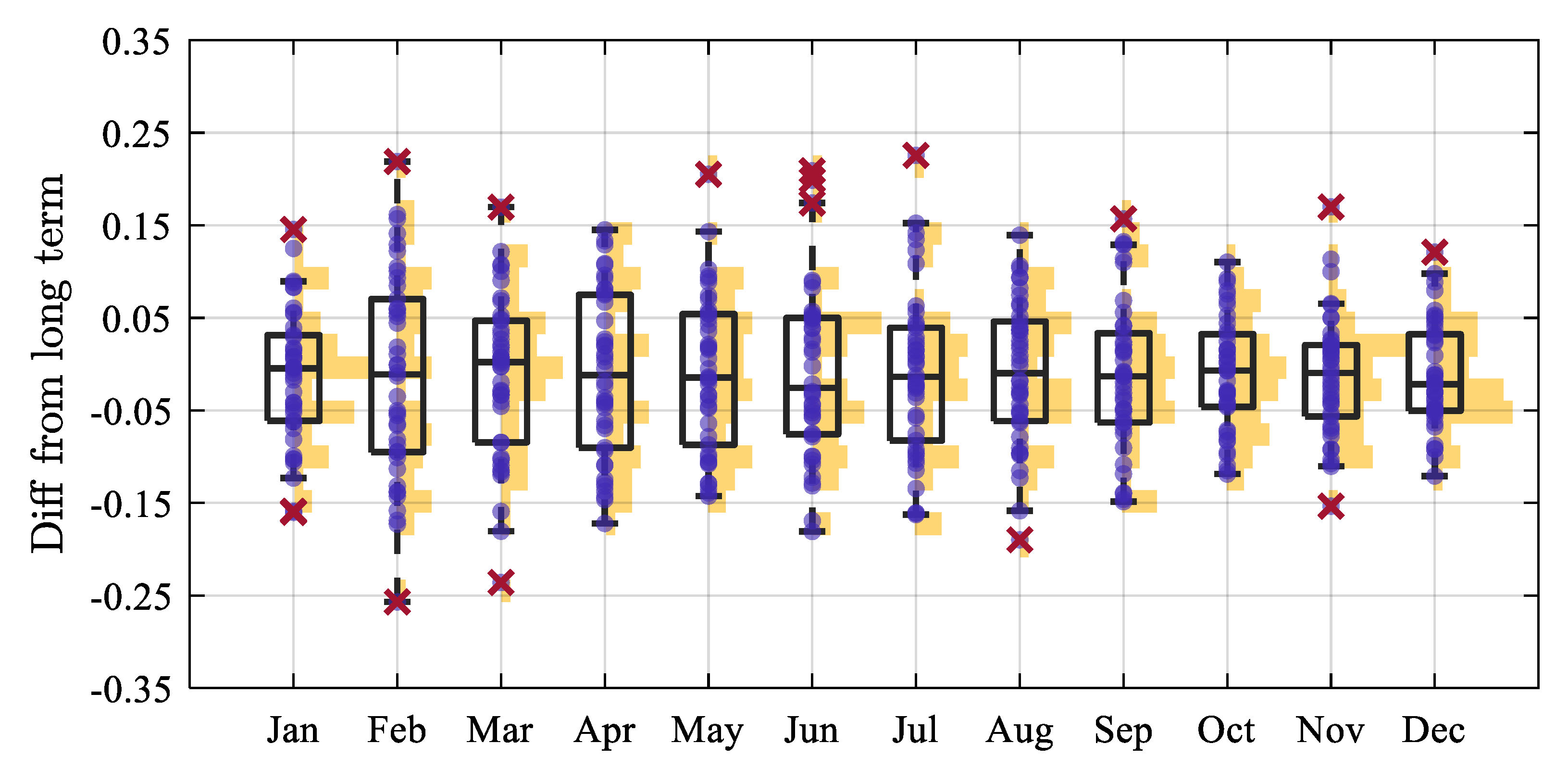
Figure 4.
The WS of the yearly weather data that are determined by (a) DBT only, (b) GSR only, and (c) GSR+DBT, given as purple dots. The yellow bars represent the occurrence distribution. The differences between the yearly and long-term weather data are calculated without absolute values. The red crosses stand for the extreme-weather months that are identified by the Z-score method.
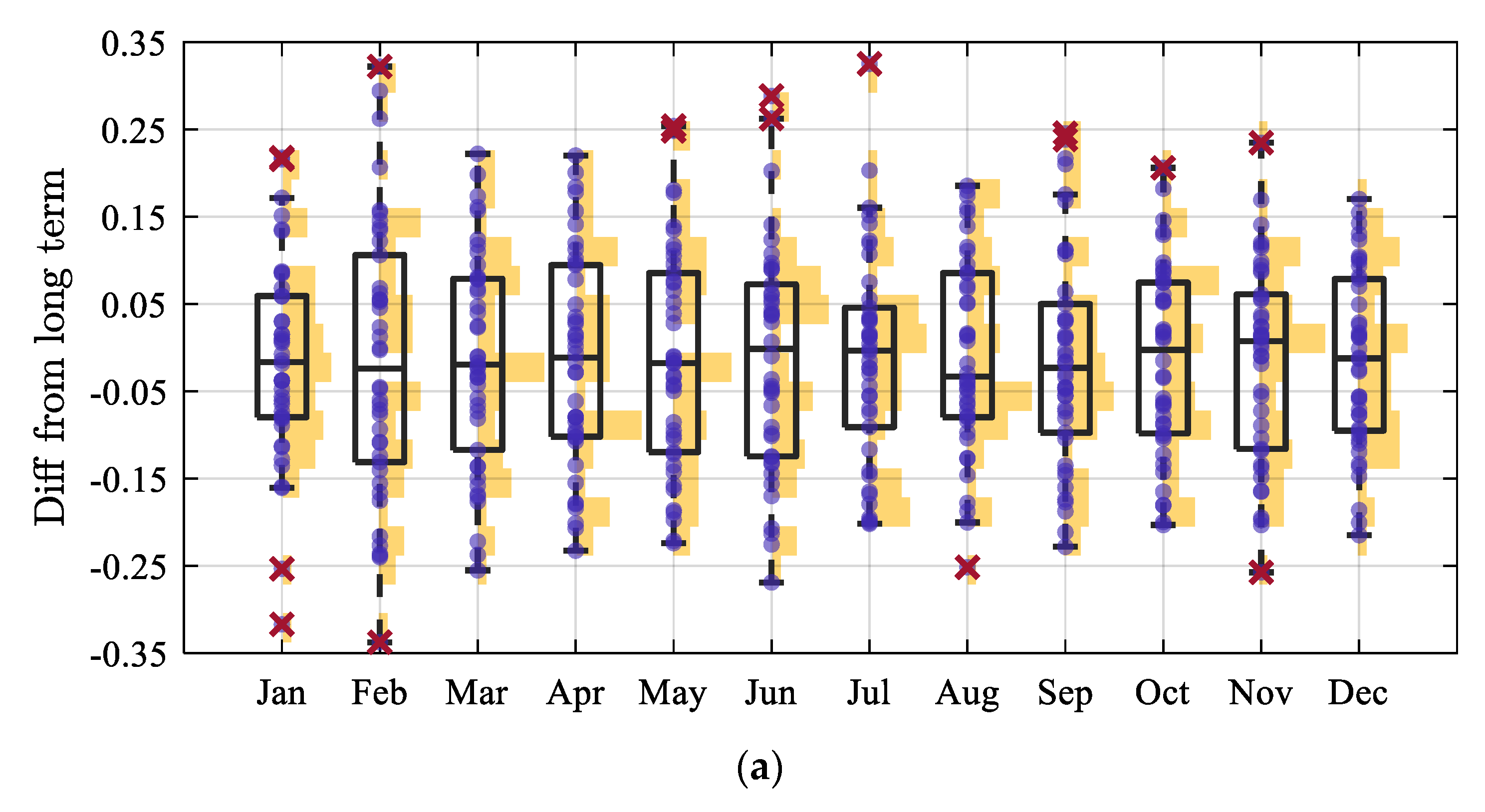

Figure 5.
Pearson auto-correlation coefficient ρ of the monthly WS values over the 42 years. The ρ values are given as the purple dots, and their occurrences are given as the yellow bars.
Figure 5.
Pearson auto-correlation coefficient ρ of the monthly WS values over the 42 years. The ρ values are given as the purple dots, and their occurrences are given as the yellow bars.
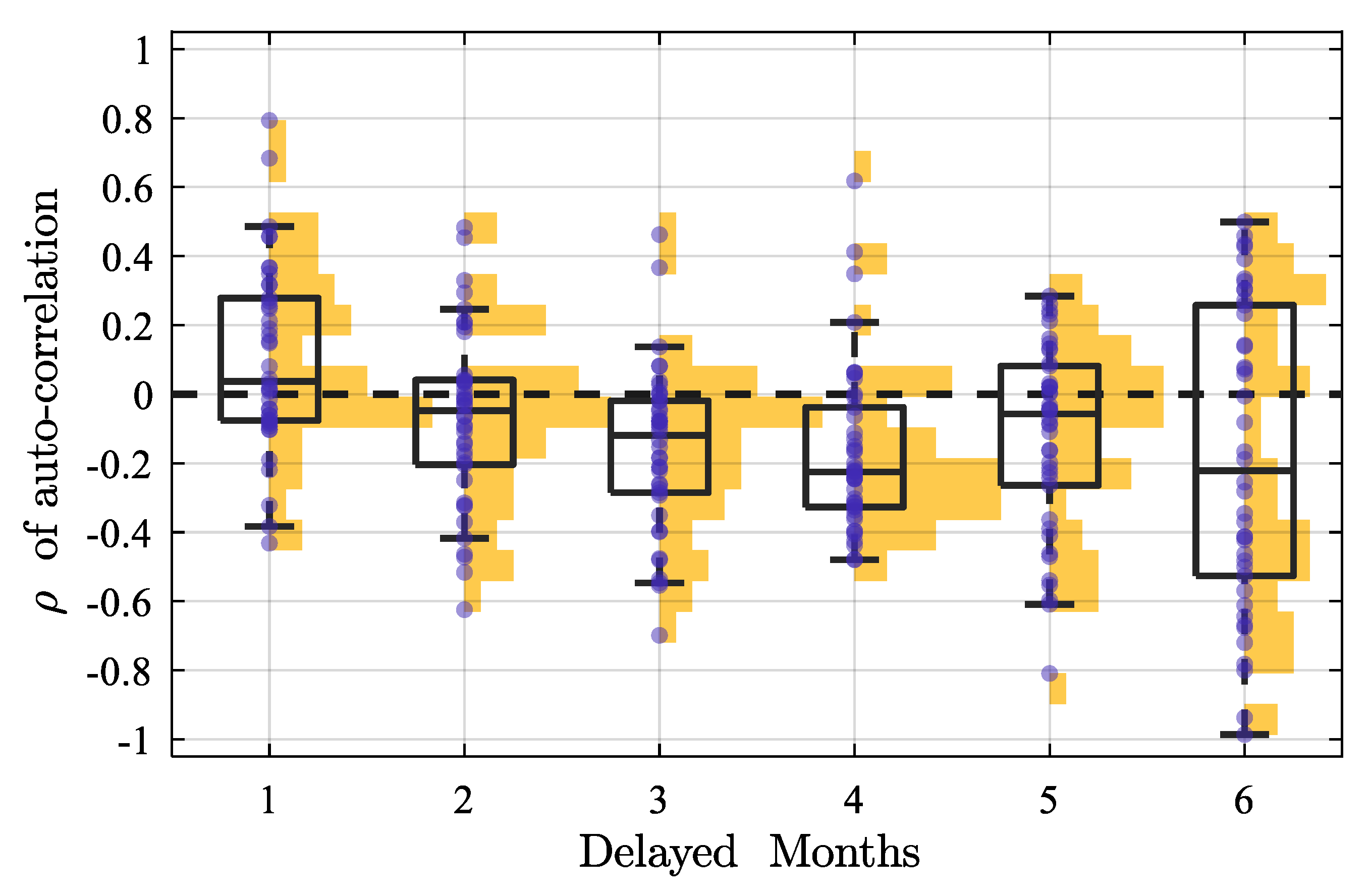
Figure 6.
(a) The monthly cooling demands of the typical building under the various warm and cool weather conditions, according to “All” climatic variables in Table 1; The difference of the untypical EWY, NEWY, and CY from the TMY in terms of cooling demands for (b) warm and (c) cool cases.
Figure 6.
(a) The monthly cooling demands of the typical building under the various warm and cool weather conditions, according to “All” climatic variables in Table 1; The difference of the untypical EWY, NEWY, and CY from the TMY in terms of cooling demands for (b) warm and (c) cool cases.
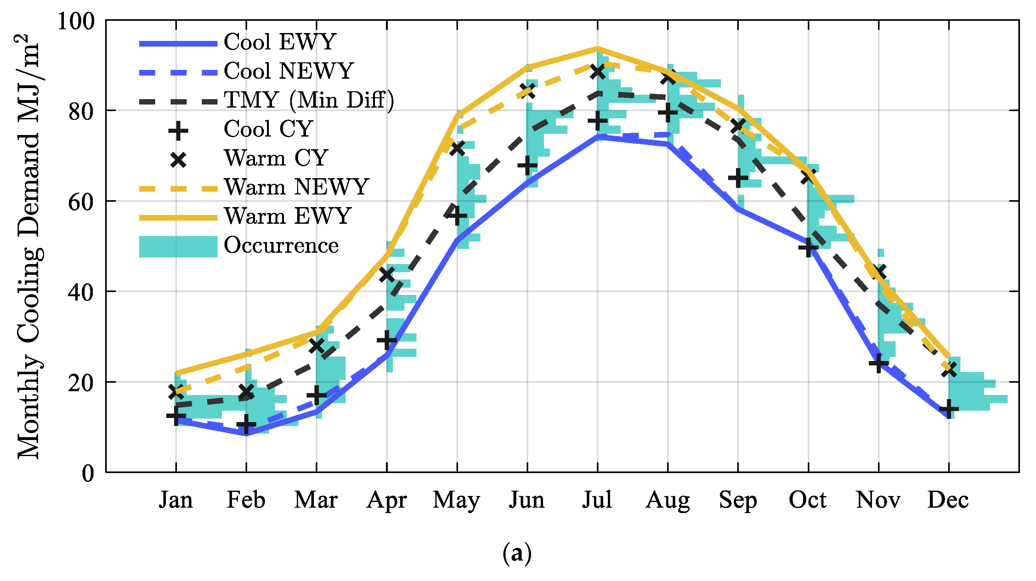
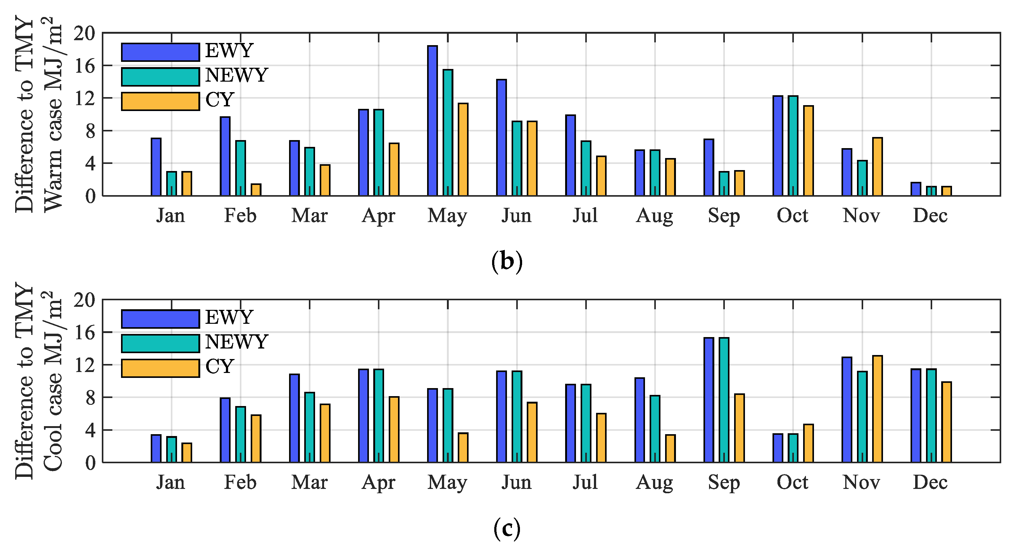
Figure 7.
(a) Cooling demands of the buildings under the warmer-than-TMY weather conditions that are identified using DBT only, GSR only, or DBT and GSR (R&T); The difference between identifying weather conditions by “All” and a part of the weather data (DBT only and DBT+GSR), as well as the demands of cooling for (b) the near-extreme warm weather year, NEWY and (c) the common warm year, CY.
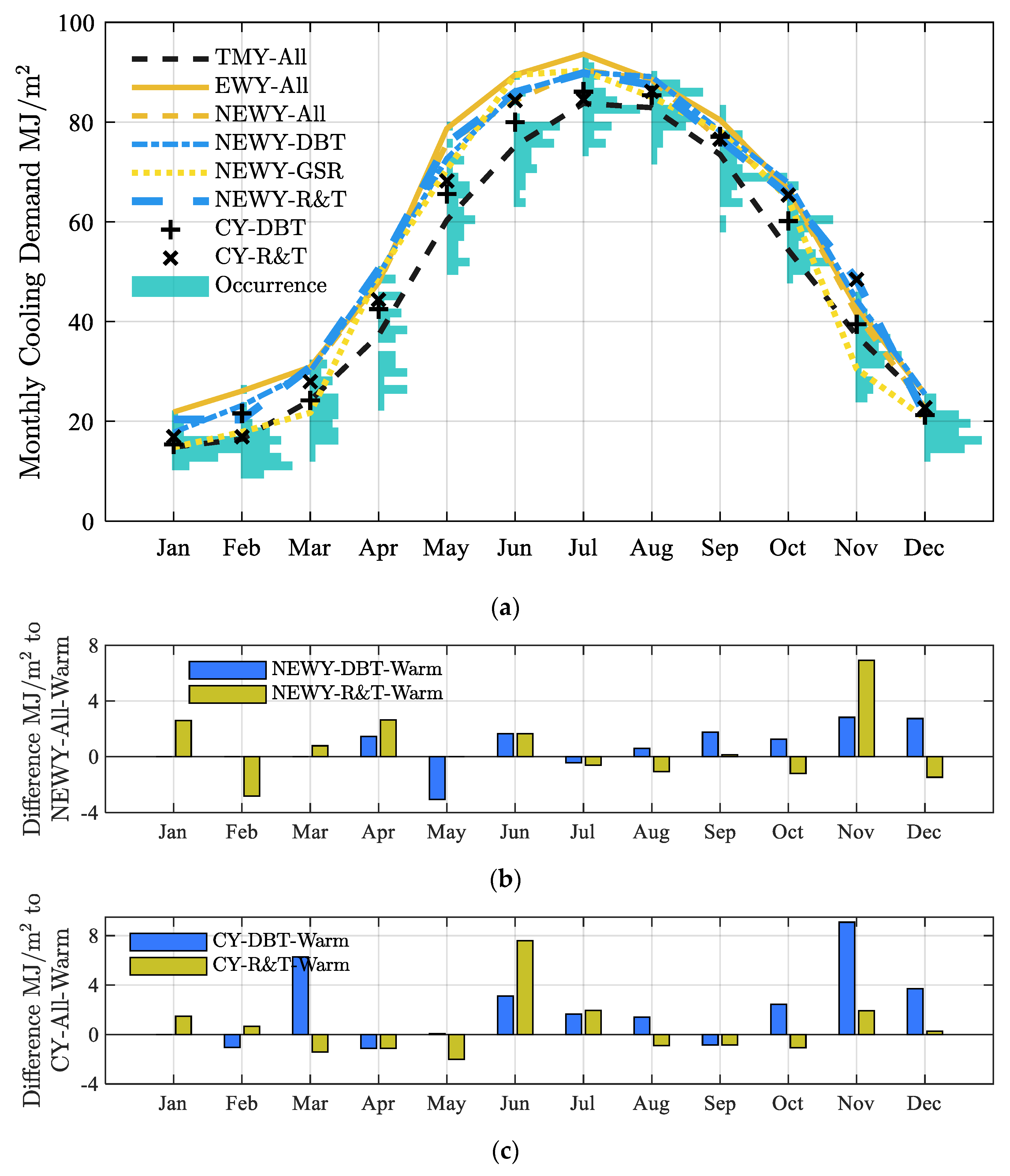
Figure 8.
(a) Cooling demands of the buildings under the cooler-than-TMY weather conditions that are identified using DBT only, GSR only, or DBT and GSR (R&T); The difference between identifying weather conditions by “All” and a part of the weather data (DBT only, and DBT+GSR), as the demands of cooling for (b) the near-extreme warm weather year, NEWY and (c) the common warm year, CY.

Figure 9.
The differences between the various untypical weather conditions and the TMY in the cooling demands.
Figure 9.
The differences between the various untypical weather conditions and the TMY in the cooling demands.
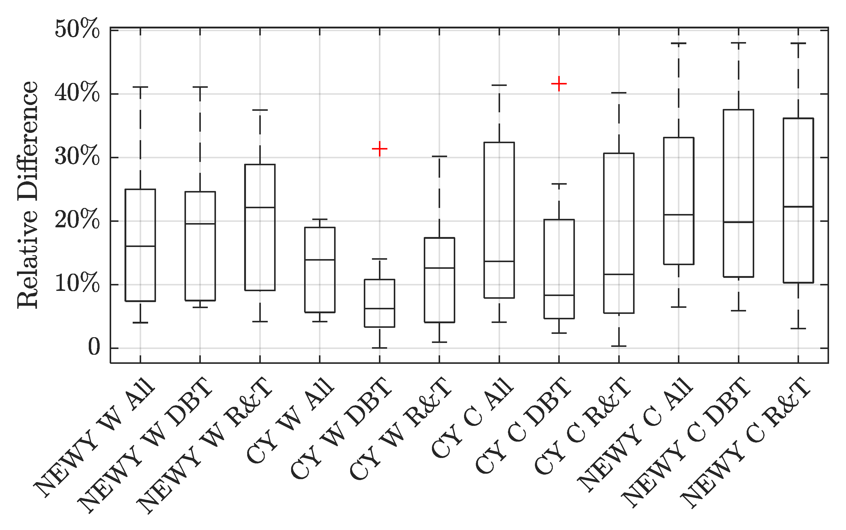
Figure 10.
Cooling demands under various weather conditions from Jul to Aug in a hot summer.

Table 1.
Weights of the weather variables for identifying the typical and extreme conditions.
| DBT | DPT | WS | GSR | ||||||
|---|---|---|---|---|---|---|---|---|---|
| Max | Min | Avg | Max | Min | Avg | Max | Avg | ||
| All | 5% | 5% | 30% | 2.5% | 2.5% | 5% | 5% | 5% | 40% |
| GSR-only | - | - | - | - | - | - | - | - | 100% |
| DBT-only | 12.5 | 12.5% | 75% | - | - | - | - | - | - |
| GSR+DBT | 6.25% | 6.25% | 37.5% | - | - | - | - | - | 50% |
Table 2.
The load densities of occupants, artificial lighting, equipment, and fresh air.
| Area Type | Floor Area per Person (m2/Person) | Fresh Air (L/s/Person) | Artificial Lighting (W/m2) | Equipment (W/m2) | Infiltration Rate (Air Change per Hour) |
|---|---|---|---|---|---|
| Office | 8 | 8 | 15 | 25 | 1.4 |
| Mall | 5 | 10 | 15 | 10 | 1.4 |
Table 3.
Thermal property of the building envelope.
| Material | (A) Wall | (B) Roof | ||||||||
|---|---|---|---|---|---|---|---|---|---|---|
| Mosaic Tile | Cement Render | Concrete Panel | Gypsum Plaster | Concrete Tiles | Asphalt | Cement Screed | Expanded Polystyrene | Concrete | Gypsum Plaster | |
| Thickness (m) | 0.005 | 0.01 | 0.1 | 0.01 | 0.025 | 0.02 | 0.05 | 0.05 | 0.15 | 0.01 |
| Conductivity (W/m K) | 1.5 | 0.72 | 2.16 | 0.51 | 1.1 | 1.2 | 0.72 | 0.035 | 2.16 | 0.51 |
| Specific heat (J/kg K) | 840 | 840 | 657 | 960 | 657 | 1700 | 840 | 1470 | 657 | 960 |
| Density (kg/m3) | 2500 | 1860 | 2400 | 1120 | 2100 | 2300 | 1860 | 23 | 2400 | 1120 |
| (C) Window | ||||||||||
| Thermal properties | Thermal conductivity (W/m K) | Transmittance | Reflectance (both sides) | |||||||
| Solar | Visible | Solar | Visible | |||||||
| Values | 1 W/(m K) | 0.834 | 0.899 | 0.075 | 0.083 | |||||
Disclaimer/Publisher’s Note: The statements, opinions and data contained in all publications are solely those of the individual author(s) and contributor(s) and not of MDPI and/or the editor(s). MDPI and/or the editor(s) disclaim responsibility for any injury to people or property resulting from any ideas, methods, instructions or products referred to in the content. |
© 2023 by the authors. Licensee MDPI, Basel, Switzerland. This article is an open access article distributed under the terms and conditions of the Creative Commons Attribution (CC BY) license (https://creativecommons.org/licenses/by/4.0/).
Share and Cite
MDPI and ACS Style
Lou, S.; Peng, Z.; Cai, J.; Zou, Y.; Huang, Y. Building Performance under Untypical Weather Conditions: A 40-Year Study of Hong Kong. Buildings 2023, 13, 2587. https://doi.org/10.3390/buildings13102587
AMA Style
Lou S, Peng Z, Cai J, Zou Y, Huang Y. Building Performance under Untypical Weather Conditions: A 40-Year Study of Hong Kong. Buildings. 2023; 13(10):2587. https://doi.org/10.3390/buildings13102587
Chicago/Turabian StyleLou, Siwei, Zhengjie Peng, Jilong Cai, Yukai Zou, and Yu Huang. 2023. "Building Performance under Untypical Weather Conditions: A 40-Year Study of Hong Kong" Buildings 13, no. 10: 2587. https://doi.org/10.3390/buildings13102587
Note that from the first issue of 2016, this journal uses article numbers instead of page numbers. See further details here.