How Do Different Methods for Generating Future Weather Data Affect Building Performance Simulations? A Comparative Analysis of Southern Europe

Abstract

Climate change will have a great impact on the hottest climates of southern Europe and the existing residential stock will be extremely vulnerable to these future climatic conditions. Therefore, there is an urgent need to update this building stock considering imminent global warming by applying climatic files that predict future conditions in building performance simulations. This research makes use of the two most applied tools (Meteonorm and CCWorldWeatherGen) for generating future climate hourly datasets for 2050 and 2080 in southern Spain. The results predicted for outdoor and indoor thermal conditions and cooling and heating demands are evaluated for two different scale simulation models: a test cell and a multi-family building located in southern Spain. The main aim of this work is the development of a comparative analysis of the results to highlight their potential differences and raise awareness of the influence of the climate data projection method on the simulation outcome. The results show that the projection method selected for producing future climatic files has relevant effects on the analysis of thermal comfort and energy demand, but it is considerably reduced when an annual evaluation is developed.

1. Introduction

Climate change is one of the largest concerns of present society and the scientific community. The member states of the European Union (EU) share a common climate goal with the main objective of achieving a zero-carbon economy, which is highly conditioned by the significant energy consumption of fossil fuels and the influence of new future climate scenarios [1]. According to the sixth assessment report of the Intergovernmental Panel on Climate Change (IPCC), if the current level of emissions were maintained, the global average temperature would increase by up to 4.4 °C by 2100 [2]. In addition, a notable increase in heat waves and extreme weather events is expected [3]. This situation will have a special impact on the warmer climates of southern Europe, where extreme temperatures are predicted similar to those of regions of North Africa and the Middle East with an increase in the frequency of tropical nights [4], significantly worsening thermal comfort and affecting future human health [5]. Specifically, in southern Spain, local climate change scenarios estimate that the number of days with temperatures above 35 °C (heat waves) would increase by more than 60 days throughout the 21st century [6].

The existing residential stock, obsolete and with low thermal and energy performance, will be extremely vulnerable to these future climatic conditions if an adequate retrofitting process is not carried out in the near future [7]. This imminent increase in temperatures will entail an improvement in indoor thermal conditions during the heating period, but it will be particularly worrying during the cooling period. This will not only result in increased cooling demand, energy consumption, and emissions, but will also have a serious impact on thermal comfort, heat stress [8], risk of overheating [9], energy poverty [10], and heat-related mortality [11].

Consequently, intervention strategies on this building stock should not only be considered to meet current needs but also to anticipate imminent global warming. Thus, it is necessary to apply reliable climatic files that predict future conditions in building performance simulations (BPSs) in order to assess the thermal comfort and energy efficiency of retrofitting processes in the future. While climate files commonly used in BPSs are based on typical meteorological years (TMYs), which combine 20-to-30-year historical observation data [12], climate projections are based on future scenarios and Global Climate Models (GCMs) [2].

The review carried out by Nielsen and Kolarik [13], which evaluates 47 studies that applied future weather data in BPSs in more than 160 locations, concluded that the U.K. Met-Office Hadley Center Coupled Model 3 (HadCM3) is the most frequently used GCM, which is present in 21 of the 47 studies. Nevertheless, in the Fifth Assessment Report [4], new GCMs were already define, based on the Representative Concentration Pathways (RCPs). Four possible emission developments in the absence of global warming policy were presented: RCP2.6, RCP4.5, RCP6, and RCP8.5, depending on the radiative force value range (2.6, 4.5, 6, and 8.5 W/m²). These scenarios are, respectively, considered to be low, medium, medium–high, and high-end cases of CO₂ concentrations [14].

Even though the original scenarios do not include probabilities, the high-end scenario, which is intended to be the 90th percentile of the no-policy baseline and considers an increase in the average global temperature of up to 2.6 °C for 2046–2065 and 4.8 °C for 2081–2100, has become significantly less likely to happen [15]. Yet it cannot be ruled out given deep uncertainties in the assignment of likelihoods to scenarios and the strong dependence on human choice in terms of economic and technological developments [16].

There are several methods for forecasting climate change weather data that increase the GCM resolution for its application in BPS. These methods can be classified into two main groups: statistical and dynamical downscaling [17]. The downscaling process consists of generating more precise climate information at the local scale from global-scale data (GCM), with an adequate spatial and temporal resolution to perform local or regional impact analyses.

According to Tootkaboni et al. [18], statistical downscaling, despite being a simplified approach, manages to provide adequate future weather data for comparative analysis in BPS, significantly reducing computational times, which makes the application of diverse climate change scenarios easier. This study compared the results of the use of three tools based on statistical downscaling and one based on dynamical downscaling for generating weather files for its application to the BPS of a single-family house and a multi-family building in Rome.

The review carried out by Nielsen and Kolarik [13] also states that morphing was the method for statistical downscaling most used (33% of the cases) and the CCWorldWeatherGen morphing tool was the second most used (24% of the cases). The morphing method, developed by Belcher et al. [19], is based on a mathematical transformation of the data by applying a combination of shift and stretch equations. Despite being widely employed, simplified morphing tools could lead to average errors in BPS results between 16–20% [20].

Although there are numerous previous studies that apply morphing methods in the analysis of the effect of climate change on thermal comfort and overheating risks [21], energy demand [22], identification of energy-poor households [23], and even heritage preservation in existing buildings in hot climates [24], there are hardly any studies comparing weather files obtained via different methods in the Mediterranean climate. In addition, most of the studies use output data from a single climate model [25] and many focus on the effect of climate change on air temperature, discarding the importance that other climatic variables have on building energy performance [13].

Therefore, the main novelty of this research is the use of different tools for generating future climate hourly data files, different outputs based on the object of study, and two different scale simulation models, with the aim of comparing the results and discussing the origin of differences detected. Both tools applied are based on statistical downscaling: Meteonorm and CCWorldWeatherGen, which are the most commonly used by the scientific community for BPS nowadays. The final objective of this comparative analysis is to generate awareness of the influence of the selected climate data projection method on the results obtained. For this purpose, future weather datasets for two different climate change scenarios (future periods around years 2050 and 2080) are generated and applied to the simulation models of a test cell and a multi-family building located in southern Spain. Values predicted for outdoor air temperature, relative humidity, and solar radiation are evaluated and compared, as well as the simulation results of thermal comfort, cooling, and heating demands.

2. Materials and Methods

To develop a comparative analysis, two climate data projection methods based on statistical downscaling were applied in this work using the software Meteonorm v7 and v8 (the most recent version of this tool) and CCWorldWeatherGen v1.9. Weather data for the years 2050 and 2080 as future periods for the city of Seville were generated. Both the base climate files used in the tools and the generated future climate files were applied to two energy simulation models: a test cell, representing a typical bedroom that allows a controlled environment, and a real multi-family building, representative of the southern Spain housing stock. The results of the energy simulations developed with the EnergyPlus calculation engine were analyzed in terms of thermal comfort and energy demand.

The methods applied for the climate projections, the development of simulation models, and the analysis of the thermal behavior of the case studies are detailed below.

2.1. Future Weather Data for Building Simulation

The location of Seville was selected for the development of the present study since it is one of the most representative cities of the dry and hot summers of the Mediterranean climate (“Csa” Köppen climate classification). For the development of future climate files, scenario A2 was selected from among the four scenarios (A1, A2, B1, and B2) defined by the IPCC in the Fourth Assessment Report [26], and RCP8.5 was selected as equivalent to the scenarios proposed in the Fifth Assessment Report [4]. These are the scenarios with the most severe forecast of CO₂ concentration at the end of the 21st century. Two of the tools applied in this work for climate projections use the HadCM3 climate model from the IPCC Fourth Assessment Report climate projections, and the most recent one uses the RCP8.5 scenario defined in the IPCC Fifth Assessment Report as GCM. A detailed explanation of the tools that have been used is provided as follows:

• CCWorldWeatherGen. Version 1.9 of this free online tool was used in this work, which employs the HadCM3 climate model, developed by the Sustainable Energy Research Group of the University of Southampton [27]. It uses the morphing methodology to produce EPW future weather data files from original TMY files. In this research, two data sets for the time slices 2041–2070 (2050 scenario) and 2071–2100 (2080 scenario) were generated, morphed from the International Weather for Energy Calculation (IWEC) TMY file of Seville [28].
• Meteonorm. Two versions of this software were used: v7, which employs the HadCM3 climate model, and v8, whose update involves the use of the RCP8.5 scenario. Both versions of this software were developed by Intersolar Europe [29]. This software is classified within the stochastic weather generators (another method for statistical downscaling that implements computer algorithms). These generators rely on a statistical analysis of recorded climate data to produce long synthetic weather series. The software integrates its own climate database, from which hourly weather data from Seville from 2010 to 2020 were applied to this research. For the climate change evaluation, the typical meteorological years of 2050 (time slices 2046–2065) and 2080 (2080–2099) were generated for the city of Seville.

2.2. Building Simulation Models

Two energy simulation models were developed, which are detailed below:

• Test Cell. The first model simulates the behavior of a test cell (Figure 1). This one was analyzed given that its geometry reproduces a typical bedroom space of the social residential stock in southern Spain while being a simplified but controlled and highly monitored environment. The cell consists of a brick facade facing south (U-value = 1.43 W/m²K) with a double-glazed window (U-value = 3.3 W/m²K). The rest of the cell envelope consists of highly insulated walls, a roof, and a floor, reproducing near adiabatic behavior (U-value = 0.05 W/m²K).
• This model has been calibrated and validated in previous research [30] through in situ measurements under controlled conditions and following the procedure defined in ASHRAE Guideline 14:2002 [31]. It was developed using the EnergyPlus open-access tool [32].
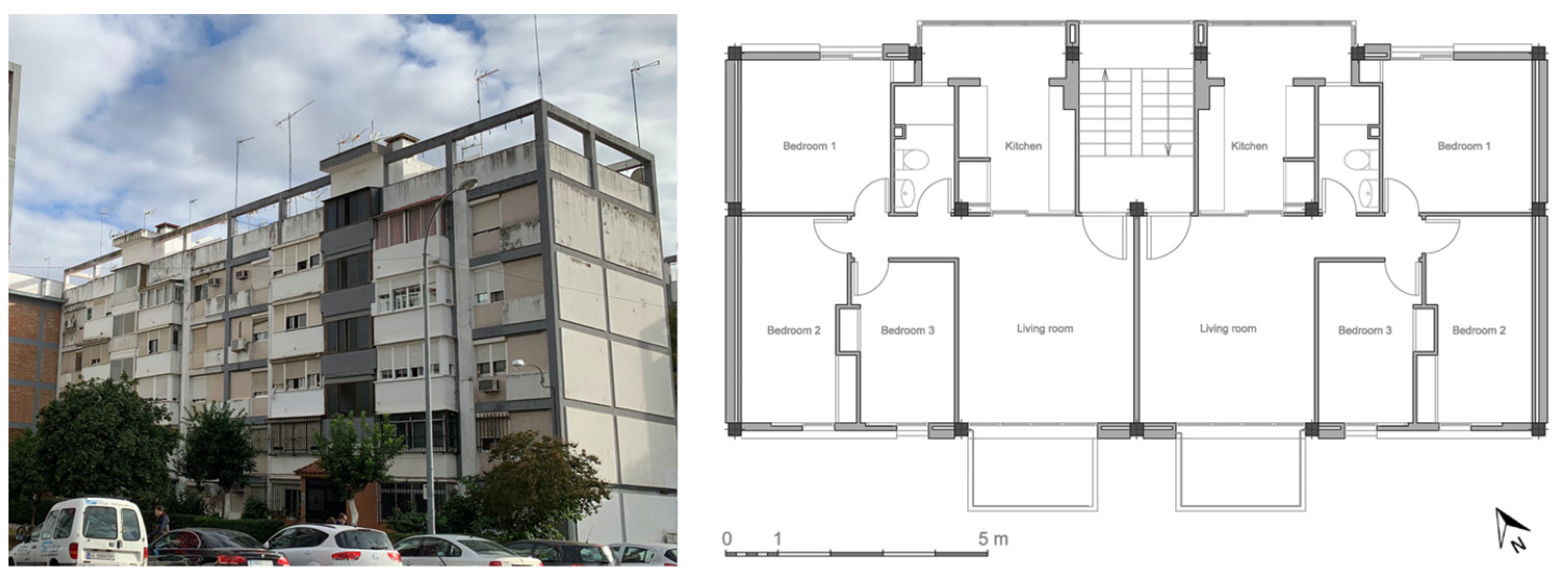
• Multi-family building. The second model used in this work represents a linear multi-family housing building built in the 1960s (Figure 2). Its morphological and constructive typology represents more than 40% of southern Spain’s social housing existing stock, being one of the most predominant building typologies of this region and, thus, a crucial real building archetype. Its brick facade has a U-value of 1.58 W/m²K, with simple-glazed windows (U-value = 5.7 W/m²K), and the roof has a U-value of 1.82 W/m²K.

This model has also been calibrated and validated in previous works [33] through in situ measurements over a full year, adopting the procedure defined in ASHRAE Guideline 14:2002 [31] (ASHRAE 2002) and also using the EnergyPlus open-access tool [32] as a simulation engine.

2.3. Adaptive Thermal Comfort and Energy Demand Assessment

For the thermal behavior assessment of the case studies under the different simulated climate scenarios, adaptive standards were considered. The scientific community considers them more suitable for free-running buildings in which users can vary their clothing level and open the windows depending on their thermal sensation [34]. According to previous research [33], the most appropriate adaptive thermal comfort standards for this climate and case study are:

• For the winter period (from December to February): EN 16798-1:2019 [35], which defines the optimum comfort temperature (Tc) according to Equation (1); in other words, it is directly dependent on outdoor temperatures. The percentage of discomfort hours is determined by considering the simulated indoor temperatures in the models that exceed the established adaptive comfort band. For the definition of the aforementioned comfort band, an acceptability range according to building category III (for a moderate level of expectation) was applied, which means a predicted percentage dissatisfied (PPD) under 15% and sets a temperature interval of +4 °C (upper comfort band limit) and −5 °C (lower comfort band limit). Thus, hourly simulation results must be obtained.

Tc = 0.33 × Ter + 18.8

(1)

Ter: running mean outdoor temperature, according to Equation (2), which must be between 10 °C and 30 °C.

Ter = (Ter1 + 0.8 × Ter2 + 0.6 × Ter3 + 0.5 × Ter4 + 0.4 × Ter5 + 0.3 × Ter6 + 0.2 × Ter7)/3.8

(2)

Ter1–Ter7: running mean outdoor temperature of the previous 1 to 7 days.

• For the summer, spring, and autumn periods (from March to November): Equation (3), defined by Barbadilla-Martín [36] for the specific case of “Mixed Mode” buildings (naturally ventilated through windows and with cooling systems for occasional use) in southern Spain. The methodology for the calculation is similar to the previous one, but in this case, the acceptability range considered corresponds to a PPD under 20% and a temperature interval of ±3.5 °C, which defines the adaptive comfort band. This leads to an updated equation for the calculation of the optimum comfort temperature (Tc).

Tc = 0.24 × Ter + 19.3

(3)

Ter: running mean outdoor temperature, according to Equation (2), between 10 °C and 30 °C.

For the energy demand estimation required in the case studies to ensure indoor comfort conditions under the different defined climate scenarios, the standard use pattern established by the current Spanish energy regulation was applied [37]. The heating and cooling set-point temperatures and use patterns are summarized in

Table 1. Heating and cooling set-point temperature patterns.

Pattern	Schedule
	23.00–7.00 h	7.00–23.00 h
Heating	17 °C	20 °C
Cooling	27 °C	25 °C

.

3. Results and Discussion

Firstly, the data for outdoor air temperature, relative humidity, and solar radiation for Seville were analyzed in each defined scenario: (1) the IWEC TMY, which is the base file used by the CCWorldWeatherGen (CCWWG) tool; (2) the 2050 and 2080 scenarios generated by CCWWG (using the HadCM3 climate model); (3) the 2020 climate data that Meteonorm v7 uses as origin; (4) the 2050 and 2080 scenarios generated by Meteonorm v7 (using the HadCM3 climate model); (5) the 2020 climate data that Meteonorm v8 uses as origin; and (6) the 2050 and 2080 scenarios generated by Meteonorm v8 (using the RCP8.5 climate model). In order to clarify the main characteristics of the different weather files applied in simulations,

Table 2. Weather file main characteristics.

Tool	CGM	Base File 1	Future Scenarios 1
CCWorldWeatherGen	HadCM3	IWEC TMY (1982–2006)	2050 (2041–2070) 2080 (2071–2100)
Meteonorm v7	HadCM3	Meteonorm database (2010–2020)	2050 (2046–2065) 2080 (2080–2099)
Meteonorm v8	RCP8.5	Meteonorm database (2010–2020)	2050 (2046–2065) 2080 (2080–2099)

¹ Generation periods.

is presented.

Once these climatic scenarios are applied to the free-running simulation models for both the test cell and the multi-family building, thermal comfort conditions were evaluated considering winter, summer, and annual periods. Finally, the heating, cooling, and total energy demands of these case studies for the different scenarios were evaluated.

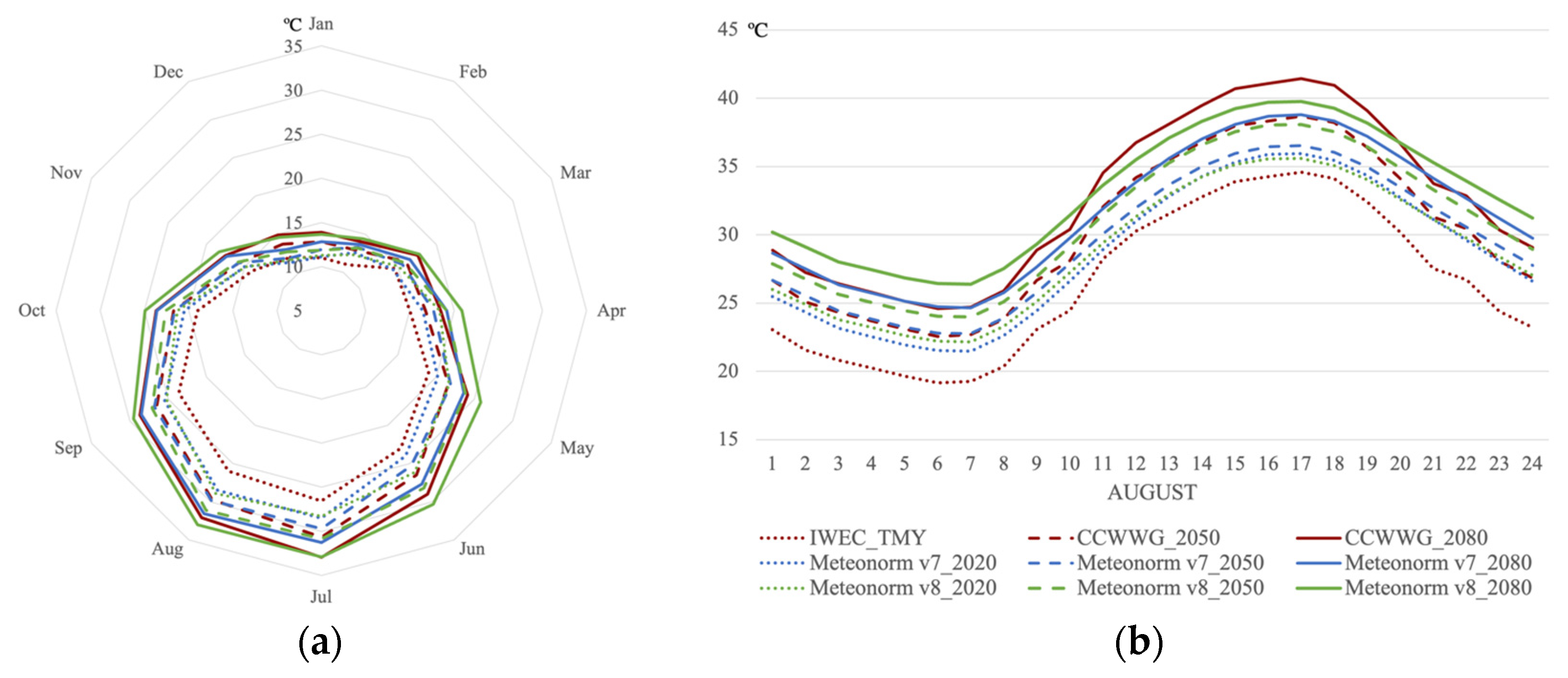
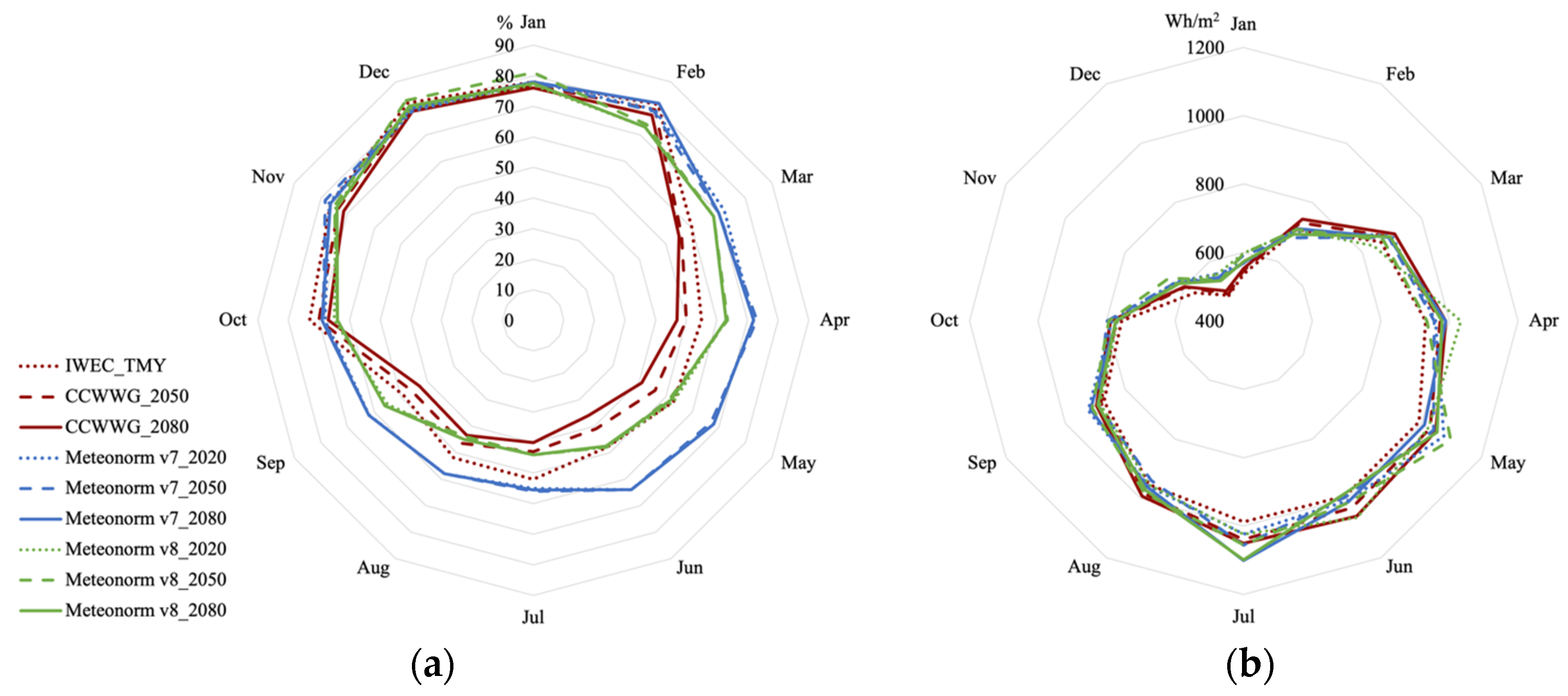
3.1. Weather Data Analysis

When comparing the values of outdoor air temperature in the different climate files (Figure 3a), it is observed that the evolution of the climate projection with the CCWWG tool is an increase in the average monthly temperature of 1.8 °C from the base file to the scenario of 2050 in winter and up to 4.1 °C in summer. The difference between the 2050 scenario and the 2080 scenario is +1.1 °C in winter and +2.5 °C in summer. In other words, the fact of using as origin a climatic file with a database from the 90s leads to a very drastic increase in the temperature projection from the TMY to the 2050 scenario.

In the case of the climatic files generated by Meteonorm v7 (HadCM3 climate model), the monthly average temperature evolution from the 2020 data to the 2050 scenario is +0.8 °C in winter and +1.3 °C in summer. Meanwhile, the difference between the 2050 and 2080 scenarios is +1 °C in winter and +1.7 °C in summer. The monthly average temperatures of the 2050 scenario are similar for the CCWWG and Meteonorm files, with the exception of December and June. In this case, the CCWWG projects a monthly average temperature of 1.8 °, which is 1.2 °C higher than Meteonorm. In the 2080 scenario, these differences are practically repeated.

For the climatic files generated by Meteonorm v8 (RCP8.5 climate model), an increase in the monthly average temperature of around 1 °C from the base file to the scenario of 2050 in winter is detected. This is represented by an increase of 2.5 °C in summer. Between 2050 and 2080, the difference is +1.8 °C in winter and +2 °C in summer. Using the same tool but with different versions, the monthly average temperature in the base file is similar throughout most of the year, except between March and June when the difference is up to +2 °C for Meteonorm v8. Regarding the 2050 scenario, the main differences are observed between April and August, with up to +2.9 °C of difference between Meteonorm v8 and v7. For the 2080 scenario, the differences between the Meteonorm v8 and v7 climate files are present in the whole year, between +0.75 °C and +2.6 °C in the monthly average temperature with the RCP8.5 model. If the monthly average temperatures of the CCWWG and Meteonorm v8 are compared, small differences are observed almost throughout the year, except for April, May, and June. During these last months, Meteonorm v8 predicts monthly average temperatures up to 2.4 °C higher than those predicted by CCWWG for both 2050 and 2080.

Particularly in August, the average outdoor air temperatures for every day of the month at each hour of the day were evaluated (Figure 3b). It is observed that the night temperatures projected by CCWWG and Meteonorm v7 are similar: between 23 and 26 °C in 2050, and between 25 and 28 °C in 2080. However, during the central hours of the day, the CCWWG tool forecasts higher temperatures than Meteonorm v7, with differences of up to +3 °C in the 2080 scenario. Meteonorm v8 predicts higher night temperatures, with a constant difference of over 1 °C for 2050 and over 1.5 °C for 2080. During the central hours of the day, Meteonorm v8 forecasts similar temperatures to the CCWWG tool for the 2050 scenario, but the forecast is around 1.5 °C lower in 2080.

When analyzing other climatic variables such as relative humidity (Figure 4a), it is detected that Meteonorm v7 and v8 estimate minimal variations in future scenarios, while CCWWG forecasts a monthly average relative humidity variation of up to −12% between the TMY and the summer months of the 2080 scenario. The relative humidity data used by Meteonorm v7 for Seville reflect a much more humid environment during the spring and summer months (with average monthly values between 60 and 70%) when compared with the climatic data used by Meteonorm v8 (with values between 45 and 65%) and CCWWG (with values between 40 and 55%).

Regarding horizontal global solar radiation (Figure 4b), very similar values are observed in the climate scenarios generated by all tools. In the future scenarios projected by CCWWG, an increase in the maximum solar radiation is observed in all months, with the greatest value in June. Yet the projection of future solar radiation follows a less constant pattern in Meteonorm v7 and v8, showing both decreases in the maximum values (in May) and increases similar to those detected in the CCWWG projections (in July).

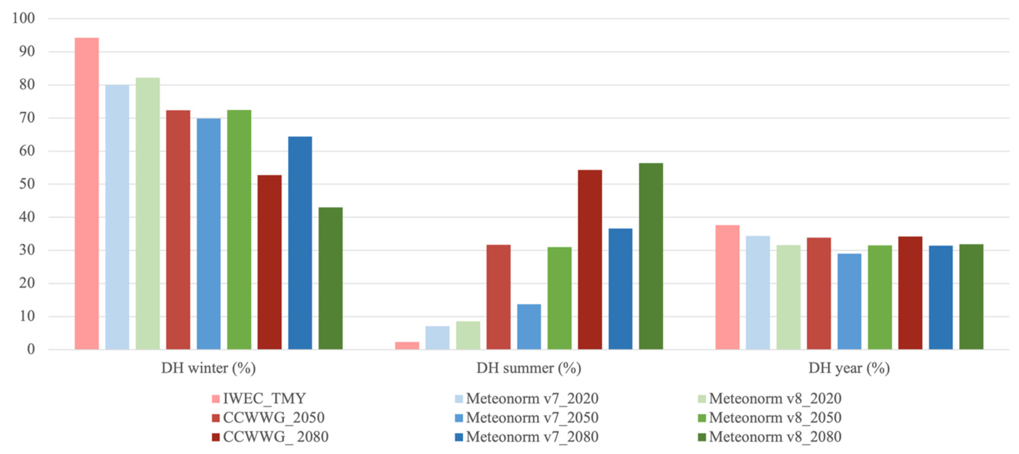
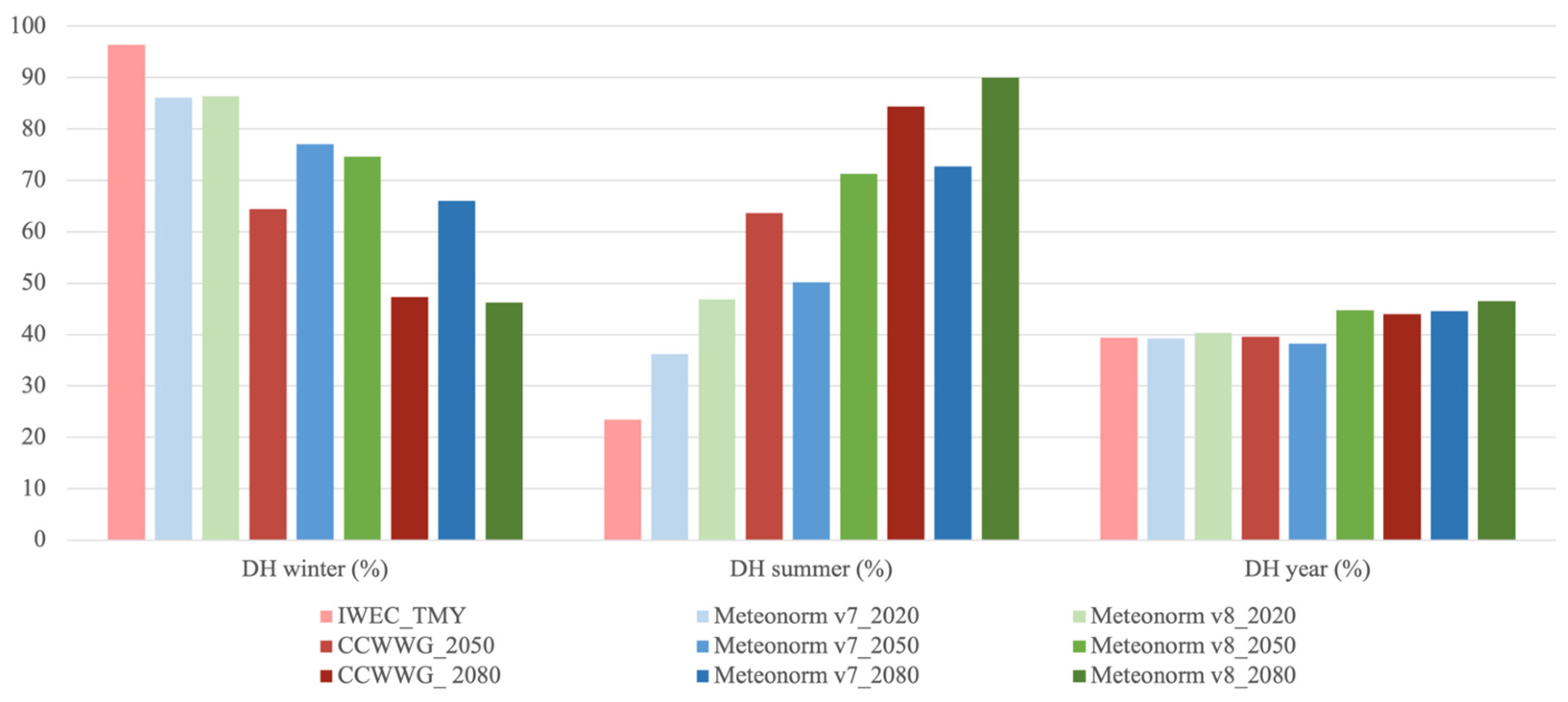
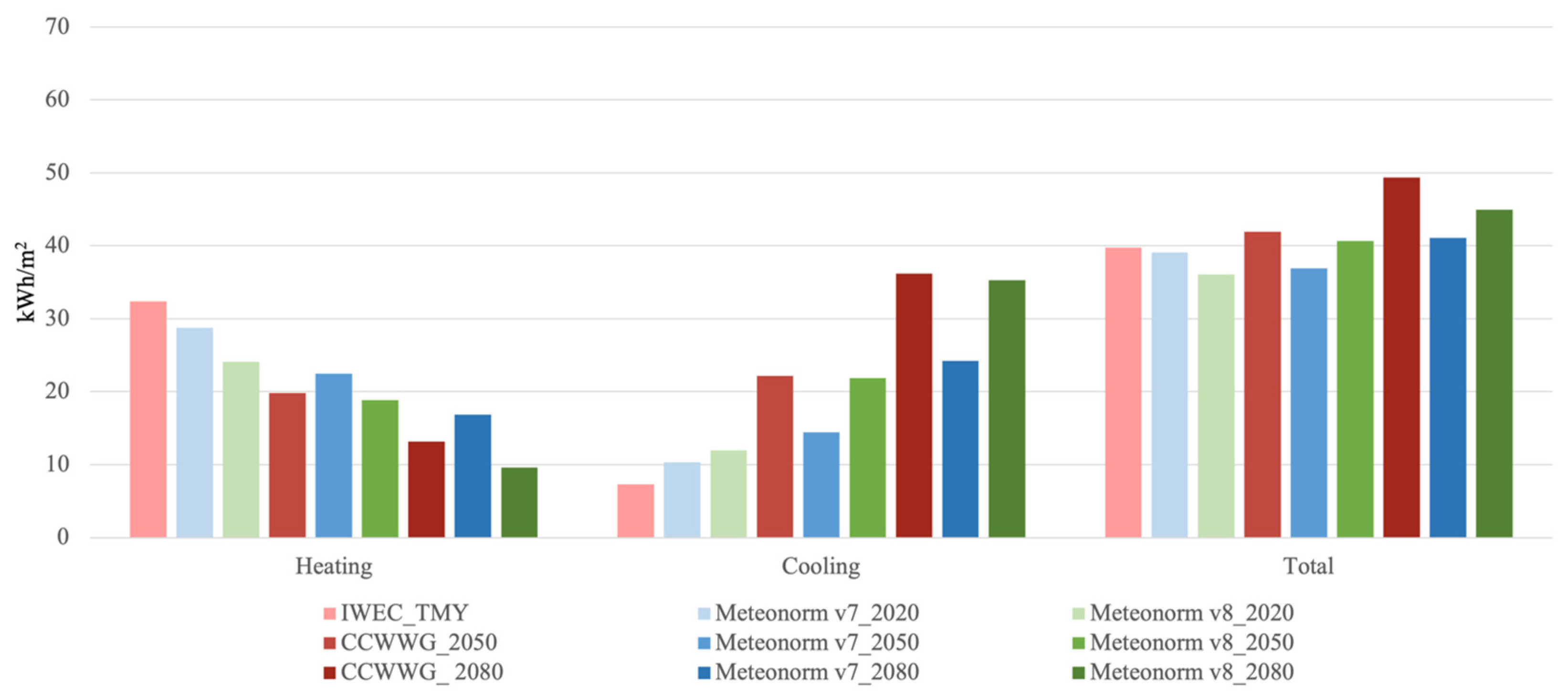
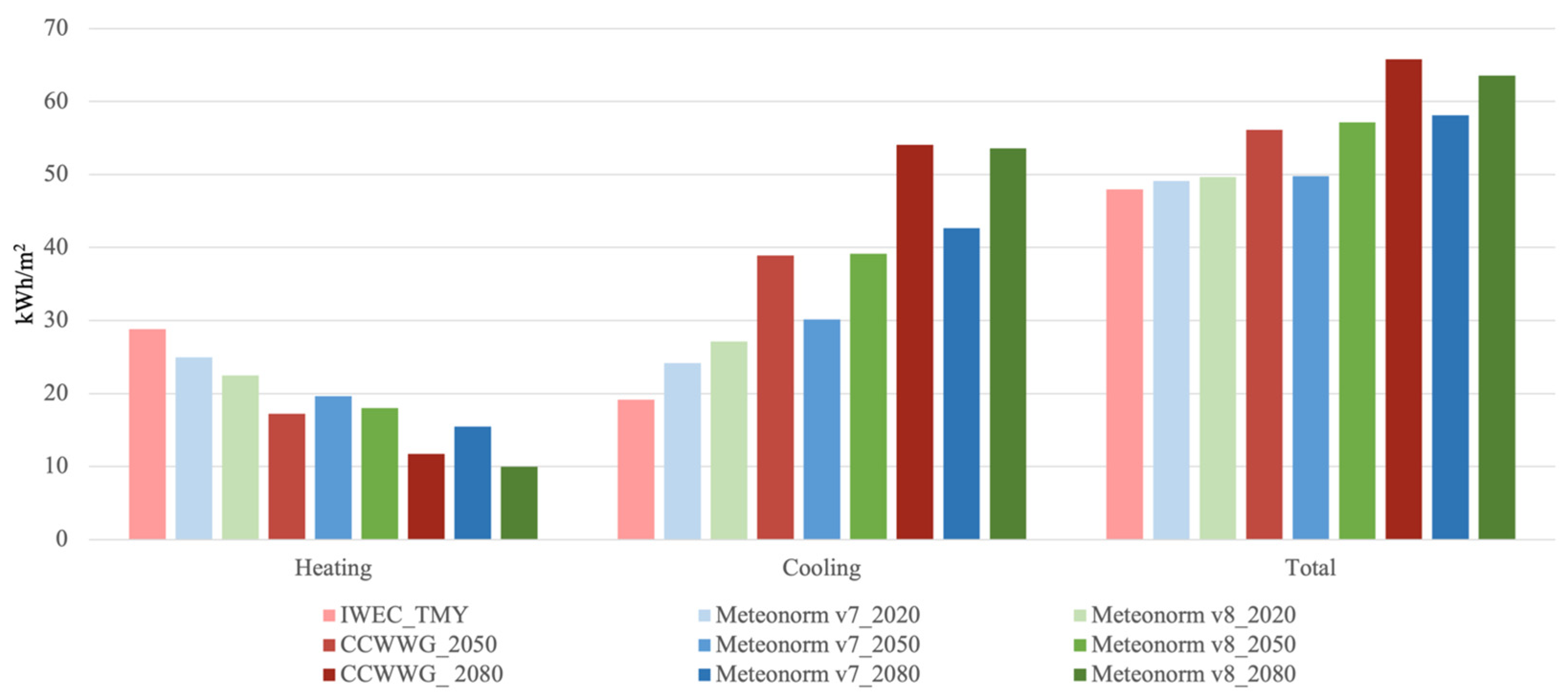
3.2. Thermal Comfort and Energy Demand Evaluation

When these climatic files are applied to the developed simulation models, it is possible to analyze the impact of the different climatic projection methods on the buildings’ thermal and energy performance. In terms of adaptive thermal comfort, in the simulation model of the test cell (Figure 5) it is observed that, as temperatures increase, the percentage of discomfort hours decreases in winter and increases in summer under future climate scenarios. With the climatic files generated by CCWWG, a greater decrease in the percentage of discomfort hours is observed in winter (41% between the TMY and the 2080 scenario) and a greater increase in summer (52% between the TMY and the 2080 scenario), since its base files have lower external temperatures. In winter, the differences in thermal comfort of the test cell are in all cases under 3% for the 2050 scenario, but up to 21% for the 2080 scenario (from 65% discomfort hours with the Meteonorm v7 climate file to 43% with Meteonorm v8). Specifically, in summer, the influence of the climate projection method on the thermal comfort of the test cell translates into differences of almost 18% in the discomfort hours, both in the 2050 scenario (from around 32% discomfort hours with CCWWG and Meteonorm v8 climate file to 14% with Meteonorm v7) and the 2080 scenario (from around 55% discomfort hours with CCWWG and Meteonorm v8 to 37% with Meteonorm v7). These differences become diluted if annual comfort is analyzed, with a maximum difference of 4.8% in the 2050 scenario.

In the multi-family building simulation model (Figure 6), the behavior of the climatic files is very similar to that observed in the test cell. The summer performance is worse than in the test cell; this may be due to its greater exposure to the outdoor environment, which in future scenarios is notably hardened. If the behavior of the different climate projection methods is compared under the building case, a greater decrease in the percentage of discomfort hours in winter (49% between the TMY and the 2080 scenario) and a greater increase in summer (61% between the TMY and the 2080 scenario) can also be detected when using the CCWWG tool compared with the Meteonorm software. During winter, the maximum difference in the thermal comfort of the building is around 13% for the 2050 scenario (with similar results for Meteonorm v7 and v8) and 19% for the 2080 scenario (with similar results for CCWWG and Meteonorm v8). Meanwhile, in summer, the influence of the climate projection method entails differences of up to 21% in the discomfort hours in the 2050 scenario (from 71% discomfort hours with the Meteonorm v8 climate file to 50% with Meteonorm v7) and 17% in the 2080 scenario (from 90% discomfort hours with the Meteonorm v8 climate file to 73% with Meteonorm v7). Analyzing annual comfort, the differences between the projection methods are greatly reduced up to a maximum of 6.5% for the 2050 scenario between the Meteonorm v8 and v7 projection methods. The greater increase in temperatures estimated by CCWWG and Meteonorm v8 makes the DH lower in winter but higher in summer compared with Meteonorm v7, which balanced the differences in annual values between all methods.

In terms of energy demand, the results are parallel in the simulation models of the test cell (Figure 7) and the multi-family building (Figure 8). Since the temperature increases, the heating demand decreases and the cooling demand increases in future climate scenarios. In almost all scenarios, the annual demand increases under future projections, except for the 2050 scenario projected by Meteonorm v7. In this case, annual demand is maintained (building model) and even slightly decreases (test cell model) in contrast to 2020. This is due to the fact that in the Meteonorm v7 2050 projection, the heating demand reduction is more relevant than the cooling demand increment; however, in the 2080 scenario, global warming gains importance and annual demand worsens.

For the heating demand, the influence of the climate projection method translates into differences of up to 2.5 kWh/m² in the 2050 scenario (with similar results for CCWWG and Meteonorm v8) and up to 7 kWh/m² in the 2080 scenario, with greater demands in the models simulated with the Meteonorm v7 climate files and lower ones with Meteonorm v8. For the cooling demand, the differences are up to 8.7 kWh/m² in 2050 (also with similar results for CCWWG and Meteonorm v8) and up to 12 kWh/m² in 2080, with the greater demands in the models simulated with the CCWWG climate files and the lower ones with Meteonorm v7. Regarding annual demand, the maximum difference is around 7 kWh/m² in 2050 and 8 kWh/m² in 2080, with the greatest demand for models simulated with the CCWWG climate files and the lowest ones under Meteonorm v7.

These results are in line with previous works, such as the one developed by Tootkaboni et al. [18] in Rome. These authors found no significant differences between the BPS results with the climate files for the 2050 scenario from CCWWG and Meteonorm (considering RCP8.5) when assessing annual discomfort hours and both heating and cooling energy demand. Yet when the percentage of overheating discomfort hours is considered, the aforementioned authors reported an insignificant difference of 3%, while in the present work, the comfort analysis in summer resulted in a difference of over 7.5% in discomfort hours between CCWWG and Meteonorm v8 for the 2050 scenario. Thus, noticeable differences may be encountered under local weather conditions, especially in global-warming-sensitive areas, such as the Mediterranean region.

Also, similar differences were found by Moazami et al. [38] when analyzing outdoor environmental conditions projected by CCWWG and Meteonorm v7 for the 2050 and 2080 scenarios in the city of Geneva. CCWWG generally predicts higher outdoor air temperatures than Meteonorm v7, with differences in the extreme values of up to 5 °C, with obvious consequences on the BPS. For this reason, further research on this matter is needed in order to develop more precise methodologies while considering uncertain approaches to energy performance assessments.

It is also important to highlight that the available literature also indicates the current uncertainty of mitigation policies’ success and the urgent need for further research to be able to develop realistic risk management assessments [39]. More research is also needed on the human capacity to adapt to climate change, as this will affect the way in which thermal comfort will be evaluated in long-term assessments.

4. Conclusions

This study carries out a comparative analysis of three different methods for generating future weather data for energy simulation in southern Spain, evaluating their influence on the thermal and energy behavior of two different scale models: a test cell and a multi-family building. The results show that although CCWorldWeatherGen and Meteonorm v7 predict similar outdoor air temperatures for the 2050 and 2080 scenarios during less severe periods, these tools significantly differ when making predictions during the coolest months and the central hours of summer days, which is probably due to the fact that solar radiation values are higher. Meteonorm v8, which incorporates the RCP8.5 scenario, generally forecasts higher outdoor air temperatures during the spring season and the summer nights. Regarding relative humidity, CCWorldWeatherGen considers a much drier climate than Meteonorm v7 from March to September, while Meteonorm v8 estimates an intermediate scenario. More extreme events of high solar radiation are observed in the 2080 scenario predicted by Meteonorm v7 and v8.

Therefore, the projection method selected for producing future climatic files has notable effects on the analysis of thermal comfort and energy demand in building performance simulations. The analysis developed concludes that the differences between applying CCWorldWeatherGen, Meteonorm v7, and Meteonorm v8 can reach up to 18% in summer discomfort hours and up to 12 kWh/m² in cooling demand for a Mediterranean region. Since generally, CCWorldWeatherGen and Meteonorm v8 predict higher outdoor temperatures, this entails a higher percentage of summer discomfort hours (with differences under 7% between both tools) and cooling demand (with insignificant differences between both tools).

When an annual evaluation is carried out, these differences between the methods applied are considerably reduced. For annual thermal comfort analysis, the maximum difference (between Meteonorm v8 and v7 projection methods for 2050) is under 7%. Regarding annual energy demand, the maximum difference is detected in the 2080 scenario, in which CCWorldWeatherGen estimates 8 kWh/m² over Meteonorm v7. The results obtained also show that neither the scale of the simulation model nor the output object of study significantly affects the behavior of the climate projection method, with similar trends.

Since they are predictions of a future scenario, it is not possible to confirm which method is more reliable by comparing them with measured data. Nonetheless, based on the results and the experience of previous works, and in accordance with the literature reviewed, it is considered that CCWorldWeatherGen and Meteonorm v8 could be overestimating the effect of global warming or assuming an excessively extreme scenario with a low probability of occurrence. These are significant facts that have to be considered when assessing thermal and energy performance in buildings under future climate change projections and that may be worth further evaluation under uncertainty analysis techniques.

References

1. Oztig, L.I. Europe’s climate change policies: The Paris Agreement and beyond. Energy Sources Part B Econ. Plan. Policy 2017, 12, 917–924. [Google Scholar] [CrossRef]
2. Intergovernmental Panel on Climate Change (IPCC). Climate Change 2021: The Physical Science Basis. Contribution of Working Group I to the Sixth Assessment Report of the Intergovernmental Panel on Climate Change; Cambridge University Press: Cambridge, UK, 2021; Available online: https://www.ipcc.ch/report/ar6/wg1/downloads/report/IPCC_AR6_WGI_Full_Report.pdf (accessed on 1 August 2023).
3. Russo, S.; Dosio, A.; Graversen, R.G.; Sillmann, J.; Carrao, H.; Dunbar, M.B.; Singleton, A.; Montagna, P.; Barbola, P.; Vogt, J.V. Magnitude of extreme heat waves in present climate and their projection in a warming world. J. Geophys. Res. Atmos. 2014, 119, 12500–12512. [Google Scholar] [CrossRef]
4. Intergovernmental Panel on Climate Change (IPCC). Climate Change 2014: Synthesis Report. Contribution of Working Groups I, II and III to the Fifth Assessment Report of the Intergovernmental Panel on Climate Change; IPCC: Geneva, Switzerland, 2014. Available online: https://www.ipcc.ch/site/assets/uploads/2018/05/SYR_AR5_FINAL_full_wcover.pdf (accessed on 1 August 2023).
5. Lima, D.C.A.; Bento, V.A.; Lemos, G.; Nogueira, M.; Soares, P.M.M. A multi-variable constrained ensemble of regional climate projections under multi-scenarios for Portugal—Part II: Sectoral climate indices. Clim. Serv. 2023, 30, 100377. [Google Scholar] [CrossRef]
6. Junta Andalucía, Consejería de Medio Ambiente y Ordenación del Territorio. El Clima de Andalucía en el Siglo XXI. Escenarios Locales de Cambio Climático de Andalucía. 2015. Available online: https://www.juntadeandalucia.es/medioambiente/portal/documents/20151/428152/clima.pdf (accessed on 1 August 2023).
7. Castaño-Rosa, R.; Sherriff, G.; Solís-Guzmán, J.; Marrero, M. The validity of the index of vulnerable homes: Evidence from consumers vulnerable to energy poverty in the UK. Energy Sources Part B Econ. Plan. Policy 2020, 15, 72–91. [Google Scholar] [CrossRef]
8. Beckmann, S.K.; Hiete, M.; Beck, C. Threshold temperatures for subjective heat stress in urban apartments—Analysing nocturnal bedroom temperatures during a heat wave in Germany. Clim. Risk Manag. 2021, 32, 100286. [Google Scholar] [CrossRef]
9. Tettey, U.Y.A.; Gustavsson, L. Energy savings and overheating risk of deep energy renovation of a multi-storey residential building in a cold climate under climate change. Energy 2020, 202, 117578. [Google Scholar] [CrossRef]
10. Costa-Campi, M.T.; Jové-Llopis, E.; Trujillo-Baute, E. Energy poverty in Spain: An income approach analysis. Energy Sources Part B Econ. Plan. Policy 2019, 14, 327–340. [Google Scholar] [CrossRef]
11. Santamouris, M. Recent progress on urban overheating and heat island research. Integrated assessment of the energy, environmental, vulnerability and health impact. Synergies with the global climate change. Energy Build. 2020, 207, 109482. [Google Scholar] [CrossRef]
12. Herrera, M.; Natarajan, S.; Coley, D.A.; Kershaw, T.; Ramallo-González, A.P.; Eames, M.; Fosas, D.; Wood, M. A review of current and future weather data for building simulation. Build. Serv. Eng. Res. Technol. 2017, 38, 602–627. [Google Scholar] [CrossRef]
13. Nielsen, C.N.; Kolarik, J. Utilization of Climate Files Predicting Future Weather in Dynamic Building Performance Simulation—A review. J. Phys. Conf. Ser. 2021, 2069, 012070. [Google Scholar] [CrossRef]
14. van Vuuren, D.P.; Edmonds, J.; Kainuma, M.; Riahi, K.; Thomson, A.; Hibbard, K.; Hurtt, G.C.; Kram, T.; Krey, V.; Lamarque, J.F.; et al. The representative concentration pathways: An overview. Clim. Change 2011, 109, 5. [Google Scholar] [CrossRef]
15. Hausfather, Z.; Peters, G.P. Emissions—The ‘business as usual’ story is misleading. Nature 2020, 577, 618–620. [Google Scholar] [CrossRef] [PubMed]
16. Schwalm, C.R.; Huntzinger, D.N.; Michalak, A.M.; Schaefer, K.; Fisher, J.B.; Fang, Y.; Wei, Y. Modeling suggests fossil fuel emissions have been driving increased land carbon uptake since the turn of the 20th Century. Sci. Rep. 2020, 10, 9059. [Google Scholar] [CrossRef] [PubMed]
17. Machard, A.; Inard, C.; Alessandrini, J.M.; Pelé, C.; Ribéron, J. A Methodology for Assembling Future Weather Files Including Heatwaves for Building Thermal Simulations from the European Coordinated Regional Downscaling Experiment (EURO-CORDEX) Climate Data. Energies 2020, 13, 3424. [Google Scholar] [CrossRef]
18. Tootkaboni, M.P.; Ballarini, I.; Zinzi, M.; Corrado, V.A. Comparative Analysis of Different Future Weather Data for Building Energy Performance Simulation. Climate 2021, 9, 37. [Google Scholar] [CrossRef]
19. Belcher, S.; Hacker, J.; Powell, D. Constructing design weather data for future climates. Build. Serv. Eng. Res. Technol. 2005, 26, 49–61. [Google Scholar] [CrossRef]
20. Bravo-Dias, J.; Carrilho da Graça, G.; Soares, P.M.M. Comparison of methodologies for generation of future weather data for building thermal energy simulation. Energy Build. 2020, 206, 109556. [Google Scholar] [CrossRef]
21. Silvero, F.; Lops, C.; Montelpare, S.; Rodrigues, F. Impact assessment of climate change on buildings in Paraguay—Overheating risk under different future climate scenarios. Build. Simul. 2019, 12, 943–960. [Google Scholar] [CrossRef]
22. Cellura, M.; Guarino, F.; Longo, S.; Tumminia, G. Climate change and the building sector: Modelling and energy implications to an office building in southern Europe. Energy Sustain. Dev. 2018, 45, 46–65. [Google Scholar] [CrossRef]
23. Spiliotis, E.; Arsenopoulos, A.; Kanellou, E.; Psarras, J.; Kontogiorgos, P. A multi-sourced data based framework for assisting utilities identify energy poor households: A case-study in Greece. Energy Sources Part B Econ. Plan. Policy 2020, 15, 49–71. [Google Scholar] [CrossRef]
24. Muñoz-González, C.M.; León, A.L.; Suárez, R.; Ruiz-Jaramillo, J. Effects of future climate change on the preservation of artworks, thermal comfort and energy consumption in historic buildings. Appl. Energy 2020, 276, 115483. [Google Scholar] [CrossRef]
25. Zhai, Z.J.; Helman, J.M. Climate change: Projections and implications to building energy use. Build. Simul. 2019, 12, 585–596. [Google Scholar] [CrossRef]
26. Intergovernmental Panel on Climate Change (IPCC). Climate Change 2007: The Physical Science Basis. Contribution of Working Group I to the Fourth Assessment Report of the Intergovernmental Panel on Climate Change; Cambridge University Press: Cambridge, UK, 2007; Available online: https://www.ipcc.ch/site/assets/uploads/2020/02/ar4-wg1-sum_vol_en.pdfpdf (accessed on 1 August 2023).
27. University of Southampton. Climate Change World Weather File Generator for World-Wide Weather Data–CCWorldWeatherGen. 2022. Available online: https://energy.soton.ac.uk/ccworldweathergen/ (accessed on 1 August 2023).
28. EnergyPlus. EnergyPlus Weather Database. 2009. Available online: https://energyplus.net/weather (accessed on 1 August 2023).
29. Meteotest. Meteonorm Software v 8.1.4. 2022. Available online: https://meteonorm.meteotest.ch/en/ (accessed on 1 August 2023).
30. Calama-González, C.M.; Symonds, P.; Petrou, G.; Suárez, R.; León-Rodríguez, A.L. Bayesian calibration of building energy models for uncertainty analysis through test cells monitoring. Appl. Energy 2021, 282, 116118. [Google Scholar] [CrossRef]
31. American Society of Heating, Refrigerating and Air-Conditioned Engineers (ASHRAE). ASHRAE Guideline 14-2002 Measurement of Energy and Demand Savings; ASHRAE: Atlanta, GA, USA, 2002. [Google Scholar]
32. EnergyPlus. EnergyPlus Software v 22.2.0. 2022. Available online: https://energyplus.net/ (accessed on 1 August 2023).
33. Escandón, R.; Suárez, R.; Sendra, J.J. Field assessment of thermal comfort conditions and energy performance of social housing: The case of hot summers in the Mediterranean climate. Energy Policy 2019, 128, 377–392. [Google Scholar] [CrossRef]
34. Djongyang, N.; Tchinda, R.; Njomo, D. Thermal comfort: A review paper. Renew. Sustain. Energy Rev. 2010, 14, 2626–2640. [Google Scholar] [CrossRef]
35. European Committee for Standardization (CEN). EN 16798-1—Energy Performance of Buildings—Ventilation for Buildings—Part 1: Indoor Environmental Input Parameters for Design and Assessment of Energy Performance of Buildings Addressing Indoor Air Quality, Thermal Environment, Lighting and Acoustics—Module M1-6; CEN: Brussels, Belgium, 2019. [Google Scholar]
36. Barbadilla-Martín, E.; Salmerón, J.M.; Guadix, J.; Aparicio-Ruiz, P.; Brotas, L. Field study on adaptive thermal comfort in mixed mode office buildings in southwestern area of Spain. Build. Environ. 2017, 123, 163–175. [Google Scholar] [CrossRef]
37. Spanish Building Technical Code (CTE). Basic Document on Energy Savings; Spanish Government: Madrid, Spain, 2022. Available online: https://www.codigotecnico.org/DocumentosCTE/AhorroEnergia.html (accessed on 13 September 2023).
38. Moazami, A.; Nik, V.M.; Carlucci, S.; Geving, S. Impacts of future weather data typology on building energy performance—Investigating long-term patterns of climate change and extreme weather conditions. Appl. Energy 2019, 238, 696–720. [Google Scholar] [CrossRef]
39. Taylor, G.; Vink, S. Managing the risks of missing international climate targets. Clim. Risk Manag. 2021, 34, 100379. [Google Scholar] [CrossRef]
Figure 1. Exterior and interior views of the test cell.
Buildings 13 02385 g001
Figure 2. Exterior view and floor plan of the multi-family building.
Buildings 13 02385 g002
Figure 3. Dry bulb temperature in Seville (°C): (a) Monthly mean; (b) August hourly mean.
Buildings 13 02385 g003
Figure 4. Weather data in Seville: (a) Monthly mean relative humidity (%); (b) monthly maximum horizontal global solar radiation (Wh/m2).
Buildings 13 02385 g004
Figure 5. Discomfort hour (DH) percentage in the test cell.
Buildings 13 02385 g005
Figure 6. Discomfort hour (DH) percentage in the multi-family building.
Buildings 13 02385 g006
Figure 7. Energy demand (heating, cooling, and total) in the test cell.
Buildings 13 02385 g007
Figure 8. Energy demand (heating, cooling, and total) in the multi-family building.
Buildings 13 02385 g008