
Spatial Characteristics and Influencing Factors of Multi-Scale Urban Living Space (ULS) Carbon Emissions in Tianjin, China

1
School of Architecture and Urban Planning, Shandong Jianzhu University, Jinan 250101, China
2
School of Architectural Engineering, Tongling University, Tongling 244061, China
3
Zibo Urban Planning Design Institute Co., Ltd., Zibo 255025, China
4
School of Architecture, Tianjin University, Tianjin 300072, China
*
Author to whom correspondence should be addressed.
Buildings 2023, 13(9), 2393; https://doi.org/10.3390/buildings13092393
Submission received: 10 August 2023
/
Revised: 6 September 2023
/
Accepted: 19 September 2023
/
Published: 21 September 2023
(This article belongs to the Special Issue Sustainable Buildings and Cities)
Abstract
:Urban living space (ULS) is known to be a significant contributor to carbon emissions. However, there is a lack of studies that have considered the impact of spatial organization indexes (SOIs) of various scales on urban living space carbon emissions (ULSCE), and so far, no definitive conclusions have been reached. To address this gap, taking Tianjin as an example, the measurement methods of ULSCE and SOI at different scales were proposed, and a random forest model was constructed to explore the effects of SOI on ULSCE. The results indicated that on the district scale, Beichen had the highest carbon emissions and absorption in 2021, with carbon emissions reaching 1.43 × 10⁸ t and carbon absorption at 7.29 × 10⁵ kg. In terms of area scale, the comprehensive service area had the highest carbon emissions at 3.57 × 10⁸ t, accounting for 47.70%, while the green leisure area had the highest carbon absorption at 5.76 × 10⁵ kg, accounting for 32.33%. At the block scale, the industrial block had the highest carbon emissions at 1.82 × 10⁸ t, accounting for 54.02%, while the forest block had the highest carbon absorption at 1.25 × 10⁶ kg, accounting for 91.33%. Each SOI had varying impacts, with the industrial land ratio (ILR) having the highest order of importance at the area scale, followed by road network density (RND), residential land ratio (RLR), bus station density (BSD), public service facilities land ratio (PLR), land mixing degree (LMD), open space ratio (OSR), and commercial land ratio (CLR). ILR, RND, and RLR were particularly important, each exceeding 10%, with importance values of 50.66%, 17.79%, and 13.17%, respectively. At the block scale, building area (BA) had the highest importance, followed by building density (BD), building height (BH), land area (LA), and floor area ratio (FAR). BA and BD were particularly important, with values of 27.31% and 21.73%, respectively. This study could serve as both theoretical and practical guidance for urban planning to aid the government in developing differentiated carbon emissions reduction strategies that can mitigate the heat island effect and promote low-carbon healthy urban planning.
1. Introduction
Urban living space (ULS) serves as the primary location for human living, entertainment, and work, as well as being the major source of carbon emissions [1]. Despite occupying less than 3% of the Earth’s surface, ULS is responsible for 78% of carbon emissions and pollutants and is continually on the rise [2]. The increase in urban living space carbon emissions (ULSCE) has significantly contributed to the degradation of urban heat islands and worsened the effects of climate change [3]. Especially in the summer, the urban heat island phenomenon can significantly increase the risk of human fatalities due to thermal emergencies and necrosis [4]. Therefore, reducing ULSCE is of immense significance in combatting global warming and achieving low-carbon development [5].
ULSCE are closely related to the spatial organization index (SOI) which has been proved by studies [6]. Numerous scholars have examined the effects of SOI on ULSCE, primarily focusing on three spatial scales: district, area, and block [7]. Concerning the district scale, scholars usually utilize exponential decomposition and spatial analysis methods to investigate the effects of SOI on ULSCE. For example, Quan et al., investigated the impact of energy intensity, urban and rural public transportation sharing rates, energy structure, population size, and forest coverage rate on ULSCE, using the logarithmic mean divisia index decomposition model [8]. Han et al., proposed that the assessment of district low-carbon levels should prioritize optimizing the proportion of land-use structure, ecological preservation in areas such as farmland and forests, ecological space planning, and the interaction between land use and transportation networks [9]. Zheng et al., used multi-source data to analyze the relationship between district carbon emissions and residential area, building area, and industrial land type in Beijing and further analyzed the spatial distribution characteristics of district carbon emissions [10].
At the area scale, studies typically select a specific city as the research sample and utilize methods such as multiple linear regression or spatial regression to investigate the correlation between various sources of SOI and ULSCE. The results demonstrate that urban land-use patterns, density of road intersections, and layout of green spaces have a significant impact on ULSCE [11]. For example, Xia et al., discovered that compact, intensive, and composite land-use patterns help to reduce ULSCE and other air pollutants, whereas the expansion of construction and industrial land is not conducive to mitigating carbon emissions [12]. Combining multi-source big data, such as mobile signaling data, and points-of-interest data, Cui et al., analyze the impact of the residential and industrial land ratio and the number of public transportation stations on ULSCE at the traffic analysis zone level [13]. According to Sharifi et al., urban green spaces are widely recognized as effective measures for reducing ULSCE, and expanding green areas is beneficial for improving air quality [14]. Schweitzer et al., examined the relationship between SOI and ULSCE, indicating that indicators such as regional centrality, road connectivity, and land-use mixture can significantly impact ULSCE [15]. Carpio et al., used satellite images and the geographic information system (GIS) to analyze the relationship between population, road traffic, vegetation displacement, and the residential and commercial sector ratio and carbon emissions in the Monterrey Metropolitan area, Mexico, and took them as the key factors associated with CO2 sink loss and CO2 emissions [16].
At the block scale, software simulation and statistical analysis methods are frequently used to analyze the impacts of SOI on ULSCE [5]. For instance, Zhang et al., analyzed the influence of building shape factors and building area factors on urban block carbon emissions and then predicted the carbon emission based on the machine learning method [2]. Based on software simulation, Zhou et al., discovered that high-density building development consumes less energy under similar conditions. They found that for every 1 °C increase in the heat island intensity, the average heating energy consumption decreases by 5.04% [17]. López-Guerrero et al., conducted a study and determined that improving building density and floor area ratio and creating a compact urban space can significantly impact ULSCE [18]. Leng et al., quantitatively analyzed the impact of SOI on the carbon emissions of different types of office blocks with simulation software and found that building energy consumption was closely related to building density and the building shape coefficient. Among them, the floor area ratio is the most critical factor in saving heating energy by up to 10.820 kWh/m2/y [5]. Through a combination of energy consumption simulation and statistical analysis techniques, Xie et al., assessed the impact of SOI on the ULSCE of university dormitory blocks in Wuhan. The research findings revealed that different block types could contribute to a significant variation of up to 35.85% in ULSCE. Furthermore, ULSCE were found to be primarily influenced by three specific SOIs: the average length of the block, shape factor, and building density [19].
As shown above, the impact of SOI on ULSCE has been widely explored. However, due to the different objects and issues chosen for different studies, there remains some debate over the influence of certain SOIs such as building area, building density, land area, and building floors on ULSCE, and further empirical studies are needed. Moreover, the majority of research exclusively investigates the impacts of SOI on ULSCE at a singular level, inadequately addressing the variances in SOI consequences at diverse scales. Scale is a fundamental concept in geography, and selecting different research scales often results in variations in research findings [20,21]. Furthermore, ULSCE encounter distinct challenges across various scales. For instance, at the district scale, the focal point is on contrasting various administrative districts, whereas, at the area scale, the emphasis lies on the different proportion ratios of various block types within different areas. At the block scale, attention shifts to the variations in building shapes across various blocks. Additionally, during the implementation of spatial planning, it becomes crucial to consider the mutual exchange between different scales to accomplish multi-level collaborative low-carbon spatial planning. Hence, it is imperative to gauge and incorporate the influence of SOI on ULSCE at varying spatial scales. Specifically, there is still a large knowledge gap regarding how and to what extent SOIs affect ULSCE at different scales, to which this study contributes. To fill existing knowledge gaps, this study uses Tianjin City, China, as a case study. Firstly, the measurement methods of ULSCE and SOI at different scales are proposed. Secondly, a random forest model is constructed to explore the effects of SOI at different scales on ULSCE. This study can better serve the government in formulating differentiated carbon emissions reduction strategies and support low-carbon, healthy urban planning.
2. Materials and Methods
2.1. Study Area
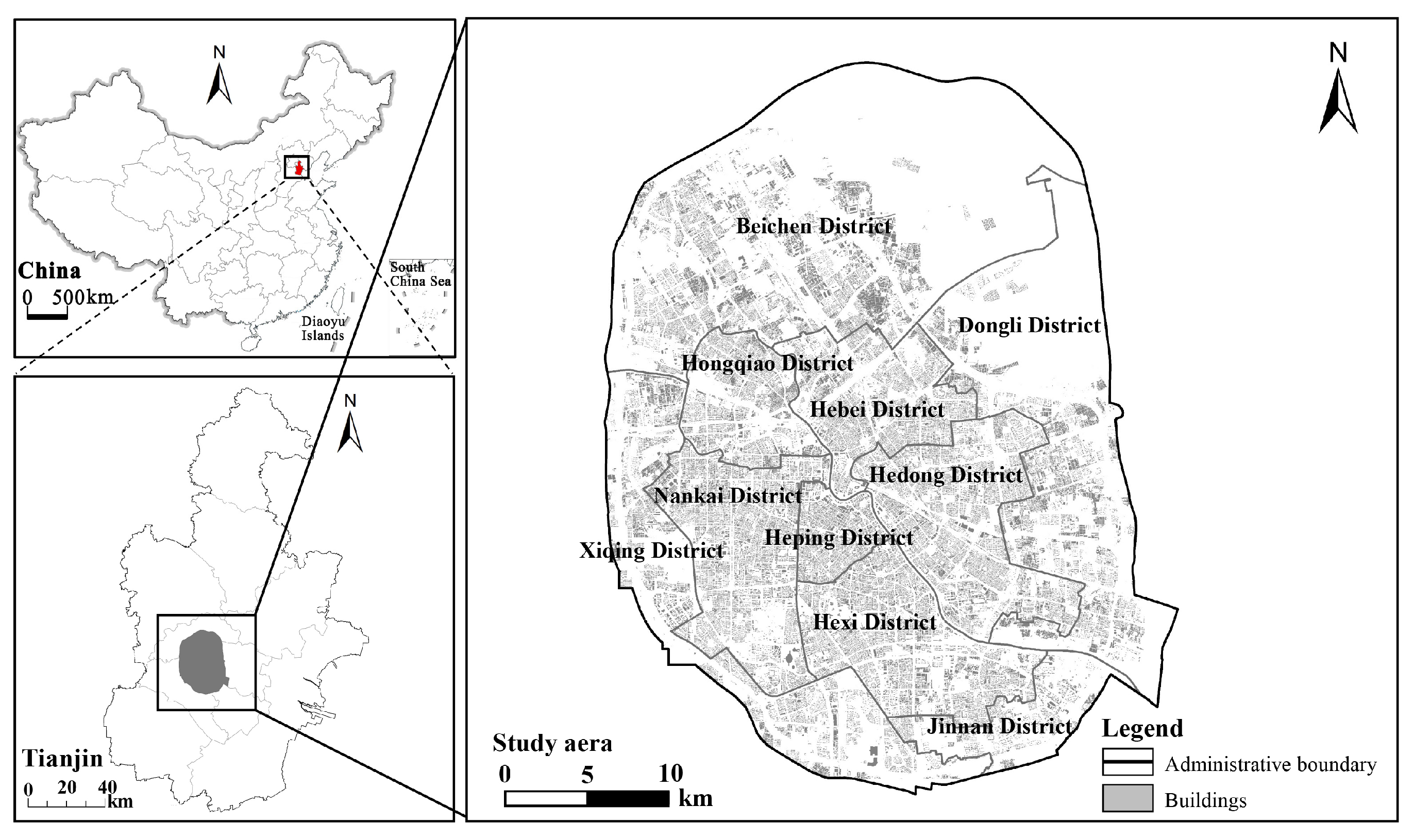
Tianjin (38°34′–40°15′ N, 116°43′–118°04′ E) is located in North China. By the end of 2022, Tianjin’s total area encompassed 11,917 km2, with a permanent population of 13.63 million and an urbanization rate of 98.76%. It governs 16 districts comprising Binhai, Heping, Hedong, Hexi, Nankai, Hebei, Hongqiao, Dongli, Xiqing, Jinnan, Beichen, Wuqing, Baodi, Jinghai, Ninghe, and Jizhou. Among these, the central urban area includes six districts in the city and four surrounding it, constituting not only the core area of urban development but also the coverage of scale in the study. The six districts in the city are Heping, Hexi, Nankai, Hebei, Hongqiao, and Hedong. The four districts surrounding the city are Beichen, Xiqing, Jinnan, and Dongli. Tianjin has always been a classic resource-based city with high energy consumption and carbon emissions, presenting a pressing need and tremendous potential for low-carbon transformation and development. Hence, selecting Tianjin as the study area showcases its typicality (Figure 1).
2.2. Research Data
The multi-source data utilized comprises (1) the 2021 Tianjin Statistical Yearbook, which primarily presents the energy consumption and other economic and social data of Tianjin, (2) point of interest (POI) data, (3) road system data, (4) block type data, obtained from the Tianjin Planning and Natural Resources Bureau, and (5) building data (Table 1).
2.3. Methods
The entire process of analysis includes the calculation of ULSCE, variable extraction of SOI, statistical analyses, and machine learning method. Firstly, the carbon emission coefficients method was used to calculate the ULSCE. Secondly, the SOIs were calculated by defining the measurement methods. Thirdly, the Spearman correlation coefficient method was adopted to examine the correlation between different types of SOIs and ULSCE. Lastly, the random forest method was utilized to analyze the effects of different types of SOIs on ULSCE at various scales.
2.3.1. Define the Measurement Methods of ULSCE and SOI
- ULSCE Measurement Methods
ULS is a spatial carrier that carries various residents’ activities and is the spatial projection of the daily activities of urban residents in various places, including residential space, leisure space, consumption space, work space, public service space, etc. Ji et al., introduce a measure of ULS that quantifies a series of concentric circles radiating from the bedroom, including bedrooms, residences, groups, blocks, areas, and administrative districts [22]. The concepts of ULS and urban construction land are different. On one hand, urban construction land only refers to residential land, industrial land, commercial land, road land, green land, etc., which does not have scale connotation and only focuses on different types. However, the ULS is similar to the living circle, which can be divided into different scales according to the size of the activity range. Among them, the determination criteria for blocks mainly correspond to land-use patches, with 44,138 blocks (Figure 2a). The determination criteria for areas are determined based on the zoning determined in the Master Plan of Tianjin Territorial Space, with 1683 areas (Figure 2b). On the other hand, in terms of type division, although block-scale ULS corresponds to urban construction land, area-scale ULS contains a variety of urban construction land types and has richer connotations. Therefore, referring to the studies of Zhang et al. [23], this study first classifies ULSCE into three major categories at the block scale for calculation, namely, industrial, road traffic, and others. Secondly, the district and area scales are summarized according to the types of the included areas and blocks, respectively. Lastly, different methods are used based on the carbon-emissions-influencing factors as allocation parameters (Figure 3).
Among them, the industrial emissions measurement method is expressed in Equations (1) and (2).
where is the carbon emissions of enterprise i of industry j, and is the total carbon emissions of industry j. is the energy consumption of enterprise i of industry j, and is the total energy consumption of industry j.
where AD is electricity consumption (kW h), EF is carbon emissions coefficient (CO2/kW h), and the value is 1.246 kg CO2/kW h.
The road traffic emissions measurement method is expressed in Equations (3) and (4) [24].
where is the carbon emissions of segment i of the road grade j, is the total carbon emissions of the road system, is the area of segment i of the road grade j, is the total area of the road grade j, and is the proportion of carbon emissions in total traffic emissions of grade j.
where is the total area of the road grade j, and is the traffic flow of the road grade j. This study divides road grades into three categories: regional road, urban road, and rural road. Among them, the traffic flow of regional road is 4500 vehicles/h, the traffic flow of urban road is 2067 vehicles/h, and the traffic flow of rural road is 500 vehicles/h [23].
Agricultural, residential, comprehensive service, commercial, other, etc., carbon emissions comprise a significant portion of overall emissions, with a concentrated spatial distribution, high continuity, and a consistent calculation method [25]. For this reason, these emissions are categorized as other types of carbon emissions [26]. The other emissions measurement method is expressed in Equation (5) [27].
where is the carbon emissions of block i of urban residential block, rural residential block, commercial block, public management and public service block, etc. is the total carbon emissions of urban residential block, rural residential block, commercial block, public management and public service block, etc. is the building area of block i.
The agricultural emissions measurement method is expressed in Equation (6) [28].
where is the carbon emissions of block i of agricultural block, is the carbon emissions coefficient of agricultural block, and is the area of agricultural block i.
The carbon absorption system comprises forest blocks, grassland blocks, water blocks, and vacant blocks. The ecological absorption measurement method is expressed in Equation (7) [29].
where is the carbon absorption of block i, and is the carbon absorption coefficient of block i. is the area of block i. is sourced from the 2021 Tianjin Statistical Yearbook and Tianjin Territorial Space Planning. is quoted from the IPCC. The carbon absorption coefficient of forest block, grassland (green) block, water (wet), and vacant block are 0.6125 tCO2/hm2·a, 0.0205 tCO2/hm2·a, 0.0253 tCO2/hm2.a, and 0.005 tCO2/hm2.a, respectively [26].
- SOI Measurement Methods
In compliance with national land planning and control guidelines, in conjunction with relevant literature research, expert interviews, and comparative analysis of multiple types of block surveys, this study classified SOIs into two main categories: area and block, totaling 13 SOIs. The area category comprises land mixing degree (LMD), road network density (RND), residential land ratio (RLR), commercial land ratio (CLR), industrial land ratio (ILR), bus station density (BSD), open space ratio (OSR), and public service facilities land ratio (PLR). The block category encompasses floor area ratio (FAR), building area (BA), building density (BD), building height (BH), and land area (LA) (Table 2).
2.3.2. Spearman Correlation Coefficient Method
The Spearman correlation coefficient method was originally proposed by Spearman in 1904. It is a statistical analysis method that measures the direction and degree of correlation between two or more variables. The calculation formula is as follows [40]:
where ρ is the Spearman correlation coefficient; is the average value of the dataset x; is the i-th data in the dataset x; is the average value of the dataset y; is the i-th data in the dataset y. The closer the absolute value of the correlation coefficient is to 1 or −1, the stronger the correlation; the closer the absolute value of the correlation coefficient is to 0, the weaker the correlation. The results show that the absolute value of the correlation coefficient above 0.8 is a strong correlation. The absolute value of the correlation coefficient is between 0.5 and 0.8, which is a moderate correlation. The absolute value of the correlation coefficient below 0.5 is considered a weak correlation or no correlation [41].
2.3.3. Random Forest Model
The random forest model, proposed by Breiman, is a machine learning algorithm based on classification trees [42]. In comparison to GIS overlay analysis, the random forest model presents numerous advantages. Firstly, it is not restricted by dimensionality, obviating the need for data standardization. Secondly, the model possesses a high classification accuracy that can be optimized and adjusted based on limited training samples to minimize errors. Thirdly, while preserving its precision, the model performs at a swift pace, and it performs better processing high-dimensional and big data rather than low-dimensional and small data. Additionally, the model offers a weight learning mechanism, which shields against the problem of overfitting in attribute evaluations of large complex nonlinear systems, and evaluates variable importance with a potent ranking function [43]. The technique flowchart for the random forest model is shown in Figure 4.
Random forest algorithms can be implemented by using a variety of software programs, including Matlab, Python, and R languages. This study chose to build a random forest model based on Python according to data characteristics. The implementation process of random forest model was as follows:
- Bootstrap Sampling
A random forest model was constructed, with ULSCE as the dependent variable and SOI of various spatial scales as the independent variable. Bootstrap sampling was performed K times on the sample set, and the data were divided into training and test sets in a 3:7 ratio (with 30% for the test set and 70% for the training set). The training set and test set were randomly allocated by using the random forest program package in R language to ensure that the data were evenly distributed in each region. The importance of each variable is calculated using the model accuracy (R2) of the test set.
- Parameter Selection and Model Optimization
Before making a decision, the parameters of the random forest model need to be adjusted to find the optimal parameters, so that the prediction accuracy of the model can be optimized. The parameters selected in this study include n_estimators, max_depth, min_sample_leaf, max_features, criterion, and min_samples_split. In order to obtain the optimal random forest model, the mesh search parameter optimization algorithm was adopted in this study [44], and the grid search interval range of each parameter was set as shown in Table 3.
In the process of building a random forest model, two important parameters, max_features and n_estimators, will directly determine the accuracy of the model. max_features refer to the number of features selected to build each decision tree, while n_estimators represent the number of decision trees of the final built random forest. Using the R language plot package, this study can analyze model error and determine stability by examining correlation graphs as the n_estimators change. In this study, with the increase in decision trees, the error of training data showed a downward trend of repeated fluctuations. When the number of decision trees was about 20, the error dropped to a low level, and then the model fitting began to converge gradually. When n_estimators = 500, the MSE (mean square error, MSE) essentially tended to a stable state. It shows that the random forest model can explain the ULSCE to a large extent.
- Importance of SOI
The weights of each feature of each sample in the random forest model were calculated by SHAP values, and then the absolute average SHAP values of all samples on different features were calculated, which was used as the importance degree of different influencing factors of ULSCE [45]. The SHAP value quantifies the contribution of each feature to the prediction made by the model, calculates the marginal contribution of the feature added to the model, and then takes the mean, that is, the reference value of the feature, after taking into account the different marginal contributions of the feature in all the feature sequences.
3. Results
3.1. Spatial Characteristics of Carbon Emissions and Absorption
3.1.1. Spatial Distribution of District Scale Carbon Emissions and Absorption
The spatial distribution of ULSCE after allocation is depicted through the geographic information system (GIS) framework (Figure 5a). The total annual carbon emissions of each district are presented in Table 4. As of 2021, Beichen exhibits the highest carbon emissions amounting to 1.43 × 10⁸ t, representing 42.43% of the total, which is significantly higher compared to other districts, with Dongli coming in second with carbon emissions of 7.10 × 10⁷ t. Heping, on the other hand, has the lowest carbon emissions with 3.59 × 10⁶ t. Carbon emissions rank from highest to lowest as Beichen, Dongli, Xiqing, Hexi, Hebei, Hedong, Nankai, Hongqiao, Jinnan, and Heping. Notably, the carbon emissions of the six districts in the city are considerably lower than those of the four districts around the city; the combined total carbon emissions of the six districts in the city amount to 8.24 × 10⁷ t, accounting for 24.44%, while the total carbon emissions of the four districts around the city are 2.54 × 10⁸ t, representing 75.56%. On one hand, industrial areas in the four surrounding areas are developing rapidly. For example, these four districts have experienced high rates of spatial expansion over the past decade, with each district expanding by an average of 3–4 km2 ULS yearly. On the other hand, the lack of comprehensive planning and low-quality infrastructure in the four districts around the city have hindered development, resulting in a scattered and highly fragmented overall layout, which has a severe impact on the ecological natural space.
From the perspective of carbon absorption, Figure 5b illustrates the total carbon absorption of the 10 districts. Among them, Beichen exhibits the highest carbon absorption in 2021, with a value of 7.29 × 10⁵ kg, accounting for 53.17%. This value is significantly greater than that of other districts, followed by Dongli with a carbon absorption of 4.88 × 10⁵ kg, while Heping presents the lowest carbon absorption of 4.50 × 10² kg. The order of carbon absorption from highest to lowest is Beichen, Dongli, Xiqing, Jinnan, Nankai, Hexi, Hebei, Hedong, Hongqiao, and Heping. Likewise, the carbon absorption of the six districts in the city is significantly lower than that of the four districts around the city. The total carbon absorption of the six districts in the city is 2.43 × 10⁴ kg, accounting for 1.77%, while the total carbon absorption of the four districts around the city is 1.35 × 10⁶ kg, accounting for 98.23% (Table 4).
3.1.2. Spatial Distribution of Area Scale Carbon Emissions and Absorption
Figure 6a displays the total carbon emissions of the 1683 areas. Notably, the comprehensive service areas exhibit the highest carbon emissions, with a carbon emission of 3.57 × 10⁸ t, accounting for 47.70%, significantly surpassing other areas. Next, residential and living areas follow with carbon emissions of 2.32 × 10⁸ t, accounting for 30.98%. Carbon emissions rank from high to low in the following order: comprehensive service areas, residential and living areas, green leisure areas, commercial and business areas, ecological control areas, transportation areas, industrial development areas, farmland protection areas, and warehousing and logistics areas. This can indicate that the leading function of Tianjin is a comprehensive service function, emphasizing high-end leadership. Optimizing and enhancing the modern service industry, it promotes the innovative and high-end development of modern service industries such as business services, modern finance, shipping services, technological innovation, cultural and creative tourism, and the headquarters economy, as well as cultivating and developing emerging business forms. From an average carbon emissions perspective, the average carbon emissions of comprehensive service areas are the largest, which is 5.67 × 10⁶ t, followed by residential and living areas with an average carbon emission of 5.38 × 10⁵ t. From high to low, the average carbon emissions ranking is comprehensive service areas, residential and living areas, commercial and business areas, transportation areas, industrial development areas, green space leisure areas, ecological control areas, storage and logistics areas, and farmland protection areas.
The spatial distribution of carbon emissions displays a noticeable disparity. The map highlights dark areas, which correspond to regions with high carbon emissions that are predominantly situated in the outer reaches of the city. These areas exhibit an increase in emissions from the core to the periphery, and the characteristics of carbon emission circle distribution are very obvious. It is concentrated in industrial centers with a larger area, as well as surrounding areas of Tianjin University and Nankai University that serve as professional public service centers. High-emissions areas include Chailou Science Park, Rongfa Decoration City, Tiannan University, Chentangzhuang industrial Park, Shuanggang industrial Park, and Balitai industrial Park, etc. Conversely, the light-colored areas on the map indicate low-carbon-emitting regions, which are primarily situated near the urban core areas containing high population densities and human activities. However, due to the relatively dense road network and smaller partition area in the core, overall emissions remain relatively low.
In terms of carbon absorption, Figure 6b depicts the total amount of carbon absorption of 1683 districts in Tianjin. Notably, the green leisure areas exhibit the highest carbon absorption, with a total of 5.76 × 10⁵ kg, representing 32.33% of the total, surpassing other area types. The residential and living areas follow closely with a carbon absorption of 5.62 × 10⁵ kg, accounting for 31.51% of the total, and ecological control areas take the third place, sequestering 5.08 × 10⁵ kg of carbon, representing 28.52%. The ranking of carbon absorption from high to low is as follows: green leisure areas, residential and living areas, ecological control areas, industrial development areas, commercial and business areas, comprehensive service areas, farmland protection areas, transportation hub areas, and warehousing and logistics areas. This demonstrates that the establishment of green and leisure spaces in Jincheng has achieved promising outcomes. These efforts should be integrated with the “One Ring and Eleven Gardens” botanical garden chain to optimize the supply of green and leisure spaces, as well as to enhance the ecological network and park system in the core area of Tianjin. In terms of average carbon absorption, residential areas exhibit the highest average carbon absorption rate of 1.30 × 10³ kg, followed by commercial and business areas with an average carbon absorption rate of 4.14 × 10² kg. The ranking of the average carbon absorption rate from high to low is as follows: residential and living areas, commercial and business areas, comprehensive service areas, ecological control areas, green leisure areas, industrial development areas, farmland protection areas, transportation hub areas, and warehousing and logistics areas.
The spatial distribution of carbon absorption exhibits a notable imbalance. The map indicates that regions with high carbon absorption are primarily situated in the northeast of Beichen. Conversely, the light areas displayed on the map signify low carbon absorption areas that are primarily concentrated near the urban core area with the most densely populated regions and human activities. Due to the relatively dense road network in the core area, coupled with the small size of the sub-area, the overall carbon absorption rate is relatively low (Figure 6b).
3.1.3. Spatial Distribution of Block Scale Carbon Emissions and Absorption
As per the comprehensive spatial planning of Tianjin, the city has been partitioned into 44,138 blocks. Table 5 presents the complete picture of carbon emissions generated by these blocks. Amongst these blocks, the industrial blocks account for the highest carbon emissions, which amount to 1.82 × 10⁸ t, constituting 54.02% of the total emissions. This demonstrates a significant gap when compared to other block types. The residential blocks closely follow, contributing carbon emissions of 7.38 × 10⁷ t, constituting 21.86%. The ranking of carbon emissions, starting from the highest, is as follows: industrial block, residential block, urban other block, warehousing block, commercial service industry block, public management and public service block, public facility block, transportation block, village other block, special block, cultivated block, garden block, agricultural facility construction block, other block, and other block within the scope of the special block. By optimizing and reducing carbon emissions originating from industrial and residential blocks, a reduction of 75% can be achieved. The average carbon emissions vary significantly across different types of blocks, with the highest average emissions observed in industrial blocks at 7.57 × 10⁴ t followed by storage blocks with emissions averaging at 6.09 × 10⁴ t. Subsequently, the descending order of average carbon emissions is observed from industrial blocks, warehousing blocks, residential blocks, public facility blocks, other city blocks, special blocks, public management and service blocks, commercial service industry blocks, other village blocks, transportation blocks, other blocks, other blocks within the special block range, cultivated blocks, garden blocks, and agricultural facility construction blocks. The building energy consumption of public management and public service blocks is colossal, resulting in their average carbon emissions exceeding those of commercial blocks such as shopping malls, hotels, and business offices. The average carbon emission intensity of urban residential blocks is approximately twelve times greater than that of rural residential blocks. Although the average carbon emissions from arable blocks are meager, their vast coverage results in a relatively high proportion of total emissions.
The map depicts high-emission areas predominantly scattered on the outskirts of the urban area, following a trend of escalating change from the core to the periphery. These regions are primarily concentrated in larger industrial centers and the vicinities of Tiannan University, constituting specialized public service centers. Some of the specific high-emission areas include Tianjin Yitong Steel Pipe Co., Ltd., Tianjin, China and Tianjin Zhenxing Cement Co., Ltd., Tianjin, China in the Chailou Science and Technology Park, Tianjin University, and Nankai University, etc. In contrast, the light-colored regions in the figure chiefly display low-carbon emissions, clustered close to the urban core areas having the highest population and human activities. Nevertheless, the overall emissions remain relatively low owing to the comparatively more dense road network and smaller partition area in the core region (Figure 7).
Table 6 displays the cumulative carbon absorption blocks in Tianjin. The forest blocks exhibit the most substantial amount of carbon absorption, measuring 1.25 × 10⁶ kg and accounting for 91.33% of the total absorption. Subsequently, water demonstrates a carbon absorption of 5.63% × 104 kg, accounting for 4.11% of the absorption. The order of carbon absorption from highest to lowest is forest block, water block, green block, vacant block, grassland block, and wet block. In terms of average carbon absorption, forest blocks exhibit the greatest average carbon absorption of 6.45 × 10² kg, with wet blocks following suit at an average of 64.53 kg. The order of average carbon absorption from highest to lowest is forest block, wet block, green block, water block, grassland block, and vacant block.
The spatial distribution of carbon absorption exhibits a significant imbalance. The map reveals that the areas of high carbon absorption are predominantly located in the northeast region of Beichen. Conversely, the low carbon absorption regions correspond to the urban core area with the highest population density and human activity levels. However, due to the more extensive road network and smaller zoning area in the core region, the overall carbon absorption is lower (Figure 8).
3.2. Influencing Factors
This study takes the 13 calculated SOIs and ULSCE to perform the correlation analysis. The correlation analysis results are presented in Table 7. At the district scale, there exists a noteworthy correlation between various SOIs and ULSCE. Notably, RLR, CLR, ILR, BSD, and PLR display significant positive correlations with ULSCE, with ILR, RLR, RND, PLR, CLR, BSD, OSR, and LMD ranking in descending order of correlation coefficients. Conversely, RND, LMD, and OSR exhibit significant negative correlations with ULSCE. At the block scale, all SOIs are significantly positively correlated with ULSCE, with LA, BH, BA, FAR, and BD scoring highest to lowest in correlation coefficients (Table 7).
3.2.1. Area Scale
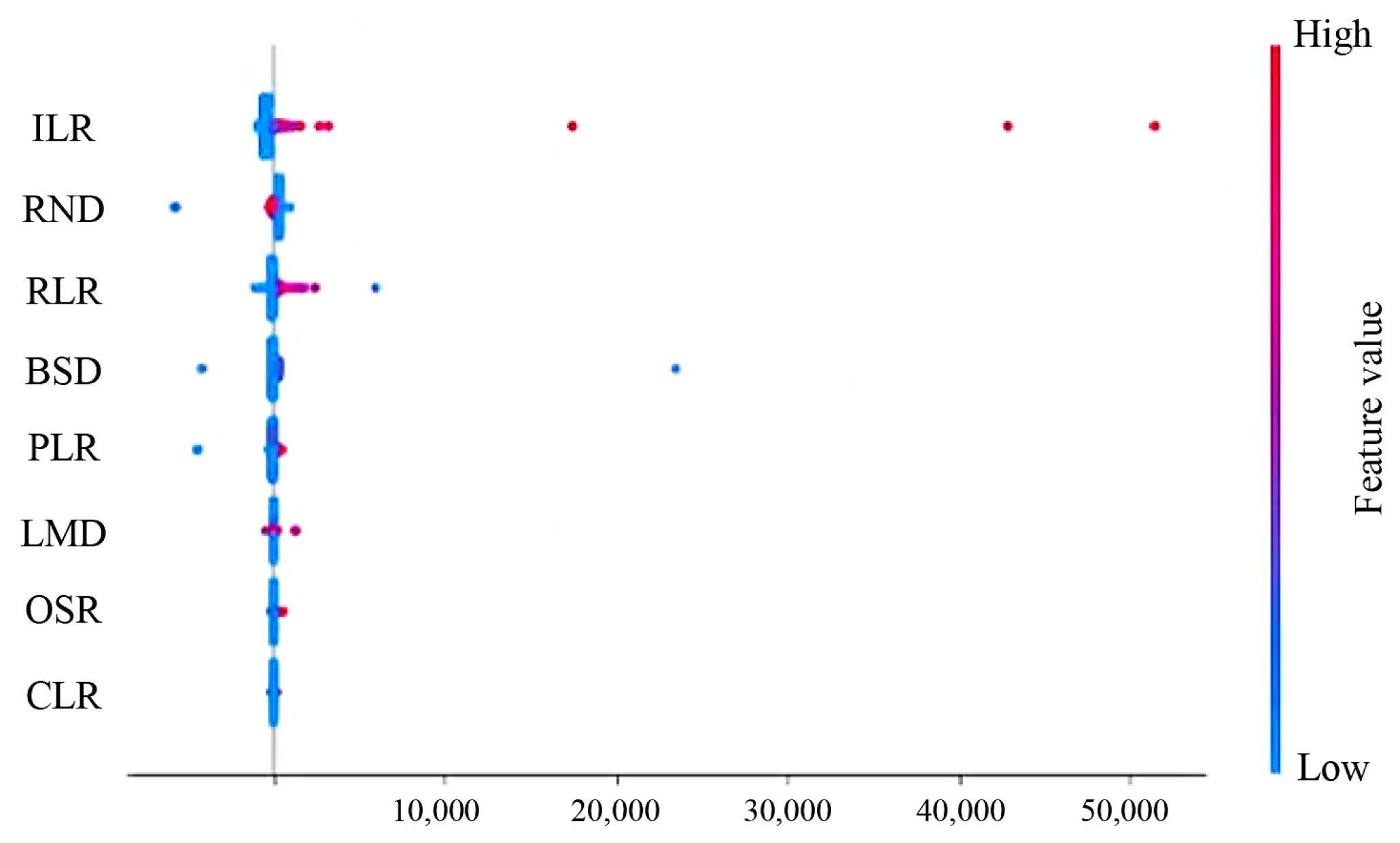
Figure 9 illustrates the global significance of key influencing factors. At the area scale, the ILR takes the highest precedence followed by RND, RLR, BSD, PSR, LMD, OSR, and CLR. Tianjin finds itself in the midst of the middle and late stages of industrialization, characterized by high energy consumption and high carbon emissions. Industrial carbon emissions stand as one of the primary sources of carbon discharge in ULS, underscoring the imperative to study low-carbon development strategies in industrial areas of great importance and value to the attainment of low-carbon development targets in Tianjin. Notably, the values of every feature of each sample are illustrated using scatter points, offering color-coded cues pertaining to the predicted impact of the different feature values. Concomitantly, the feature value distribution can be gleaned from the same graphical display.
The significance of the SOI impact on the ULSCE at the area scale was assessed. ILR, RND, and RLR all surpassed a 10% importance threshold, with percentages of 50.66%, 17.79%, and 13.17%, respectively. The cumulative importance of the three SOIs was as high as 81.62%, revealing their dominant contribution to ULSCE on the area scale. Among these, ILR had the most substantial impact on the classification outcome. LMD, CLR, and OSR recorded the lowest feature importance, with their significance levels being less than 2% individually, i.e., 1.10%, 1.10%, and 0.46%, respectively. Given the limited magnitude of OSR, it had the least effect on reducing ULSCE at the area scale. The importance of the other two indicators, BSD and PSR, was 9.84%. BSD’s significance level surpassed that of PSR and had a more considerable impact on the evaluation results (Table 8).
3.2.2. Block Scale
Figure 10 illustrates the impact of key influencing factors. At the block scale, the BA is the most influential, followed by BD, BH, LA, and FAR. This aligns with previous research findings. At this scale, building energy consumption generates the highest proportion of carbon emissions, with residential and public blocks contributing approximately 95%. The BA holds the strongest correlation with building energy consumption and carbon emissions at the block level.
The significance of SOIs affecting ULSCE at the block scale is ranked, with BA and BD having an importance of over 20%, 27.31%, and 21.73%, respectively. The combined importance of these two indicators is equally high at 49.04%, signifying that these two features hold the greatest contribution to ULSCE at the block scale. BH, LA, and FAR are three indicators with relatively low importance, and their significance stands at less than 20%, 17.92%, 17.54%, and 15.51%, respectively. Among these, BH and LA are closely ranked, are more significant than FAR, and thus contribute more to the assessment outcomes (Table 9).
4. Discussions
4.1. Impact of SOI on ULSCE
The results demonstrate that different kinds of SOIs lead to distinctively different ULSCE at different scales. However, the mechanism of the SOI configuration that affects the ULSCE according to the quantitative results needs to be explored to provide effective and scientific urban planning suggestions.
4.1.1. Impact of SOI of Area Scale on ULSCE
This study focuses on the analysis of the three SOIs that have the greatest impact at the area scale (Figure 11).
- ILR
Industrial energy consumption is the most crucial element of the urban energy consumption pattern. As a historically established industrial hub in China, the industrial areas in Tianjin are primarily located in the four districts around the city. While these industrial areas act as a significant driver and foundation of the local economy, they also face issues such as excessive energy usage, an extensive industrial mode, and environmental pollution. The study of Li et al., provides evidence for this view. Li et al., indicate that industrial areas have the highest carbon emission levels, and even zones with a high development intensity, such as residential or commercial areas, have lower carbon emission levels than industrial areas [33]. A previous study on the carbon emissions of Tianjin also proves that industrial restructuring is still a very important entry point for carbon emissions reduction [46]. Zheng et al., found that industrial structure has an energy-saving effect with diminishing marginal effects, which can achieve a reduction in carbon emissions [47]. Therefore, the reduction in carbon emissions in these districts has become a priority for Tianjin, with a focus on structural changes in the industrial structure and enhanced energy efficiency measures.
- RND
The findings of the RND and ULSCE are presented in Figure 12. As RND increases, ULSCE at the area scale exhibits an initial rise, followed by a decline, with a turning point observed between 0 and 0.2. Using 0.08 as the boundary, RND is positively correlated with ULSCE when it is less than 0.08 but negatively correlated when it is greater than 0.08. In the aspect of reasoning analysis, the ULSCE is related to transforming road network forms. Zhang et al., found that transforming a dendritic road network into a mixed road network and a polygonal road network into a grid road network can theoretically reduce ULSCE by 0.245 and 0.312 tons [48]. It is also a potential course of action for the next step. Therefore, different road network forms, intersection organization, and road density can influence the driving distance of motor vehicles, thereby increasing fuel consumption. Optimal geometric designs, appropriate road density, and a rational road network structure can indirectly reduce travel distances and traffic congestion and promote energy conservation and emission reduction [49]. In addition, to encourage the use of walking and public transport, it is recommended to limit walking distances to no more than 200 m to bus stops, which would result in more than 50% of individuals opting for public transport. In light of this, the block size of bus-oriented developments should not exceed 150 m × 150 m when walking is the primary mode of transportation. In suburban areas with lower transit network density, it is advisable to introduce bicycle transfers for buses. With cycling speeds of 10–12 km, individuals can access stations within roughly 800 km cycling for 3–5 min. To account for detours, the block size should range from 400 to 600 m. Therefore, urban planning must delve deeply into the reasons why societies are car-reliant and ensure that the needs of the people across different travel purposes are appropriately addressed. This can be achieved by increasing the road network density, creating wider isolation green belts and sufficient slow traffic space, constructing a safe slow traffic space network, and reducing carbon emissions.
- RLR
The findings of the RLR and ULSCE are presented in Figure 12. With the increase in RLR, ULSCE showed a trend of first increasing and then decreasing, with an inflection point between 0.4 and 0.6. The significance of residential blocks has always been a concern, as they are directly linked to the carbon emissions resulting from residents’ day-to-day activities such as lighting, heating, and cooking. It has been found that carbon emissions can be reduced by 35.13% through the optimization of the building monomer and landscape greening [50]. This requires further discussion on the block scale. Tianjin must, therefore, take measures to reasonably limit the expansion of residential blocks through the adjustment of urban planning, control the area dedicated to construction land, and restrict the boundaries for the future construction of ULS. Moreover, future population development trends, particularly in the central urban area, must be predicted and taken into account when imposing further limitations on the scale of residential blocks to avoid their haphazard expansion. Additionally, resident guidance on energy conservation should be strengthened, promoting energy-conscious behaviors. This may be achieved by encouraging residents to purchase energy-efficient household appliances through subsidies or price reductions.
4.1.2. Impact of SOI of Block Scale on ULSCE
This study focuses on the analysis of the two SOIs that have the greatest impact at the block scale (Figure 12).
- BA
Figure 12 displays the outcomes of BA and ULSCE. ULSCE at the block scale illustrates a pattern of initially increasing and then decreasing when the BA is within 10,000 m2. However, when the BA exceeds 10,000 m2, ULSCE at the block scale persistently increases. These findings align with the current research in this field and may differ in the specific turning points, but the overall trend is consistent [37]. This is mainly related to the influence of microclimate. For example, Wong et al., analyzed the impact of BA on carbon emissions through simulation, selecting 32 block cases with varying building areas. Their findings indicated that, under the same conditions, an increase in building area could result in a 2 °C reduction in block temperature and a 4.5% reduction in carbon emissions, but at a certain point, carbon emissions begin to increase [51]. Li et al., found that a larger BA induced a reduction in residential district carbon emissions, but the observed effect is notable at an initial increase in BA [52]. Hence, in a high-density urban environment like Tianjin, further lowering BA to reduce ULSCE should receive the attention of researchers, policymakers, and planners. Although BA is a significant indicator for quantifying land-use economics, high BA rules out high cooling or heating demand, resulting in an impact on lighting, thermal radiation, and air circulation. For instance, an excessive amount of BA increases the building surface area of the block for absorbing solar radiation, eventually affecting land cooling or heating expenditures through modifying regional microclimate. Several research studies have been carried out to examine the influence of building area on building energy consumption, such as Battista et al.’s view that building area enhancement heightens the heat island effect and therefore raises carbon emissions [53]. Liao et al., employed remote sensing data to execute a correlation analysis on the heat island effect during diverse years. Their work established that a strong positive correlation exists among building area, heat island intensity, and building energy consumption, with the correlation coefficient exceeding 0.8 [54].
- BD
In general, higher BD results in lower carbon emissions, but the overall impact is minimal. These findings are consistent with previous studies. BD reflects the spatial distribution of building entities within a ULS, influencing wind, heat, and light environments and consequently having an important impact on carbon emissions. Higher BD can lead to greater building coverage and mutual occlusion, potentially affecting the utilization of solar energy in winter and increasing building heating energy consumption. Boccalatte et al., analyzed the relationship between average plot BD and carbon emissions in 25 cities worldwide and identified building density as a key factor in carbon emissions for construction land [55]. He et al., introduced the concept of the ecological floor area ratio, verified the relationship between building energy consumption and urban spatial form, and found that as building density decreases, building energy consumption increases fractionally [56]. Yu et al., used simulation software to predict energy consumption and discovered that lower building density in a block leads to higher building energy consumption and increased carbon emissions, while higher building density results in lower carbon emissions, and there is a clear negative correlation [57].
4.2. Applications
After obtaining the aforementioned analysis results, this study proposes potential planning strategies at the area and block scales for reducing carbon emissions in Tianjin. Firstly, to ensure the low-carbon development of Tianjin, it is imperative to strengthen industrial agglomeration and inter-industry correlation. Industrial agglomeration can be achieved by constructing industrial parks and integrating dispersed factories, while simultaneously coordinating and extending the park and dispersed industries to form an industrial chain. This will strengthen the correlation between industries, meet the economic development needs of Tianjin, enhance industrial agglomeration development, and effectively reduce the level of carbon emissions [58]. Secondly, while there is a significant discrepancy between artificial land use and vegetation land demand, increasing vegetation coverage is essential, not only to minimize carbon emissions but also to improve the living environment [59]. Thirdly, the spatial characteristics of carbon emissions can provide fundamental information for constructing vector carbon emissions maps at various scales. Finally, establishing a definitive association between SOI and ULSCE can establish the foundation for future investigation, offering supplementary reinforcement for urban development and attaining carbon reduction through indicator management. Overall, incorporating the concept of low-carbon urban planning and proposing low-carbon-oriented urban planning strategies in cities are crucial for mitigating climate change and developing low-carbon cities.
4.3. Limitations and Further Improvements
What is more, there are some limitations to this study. Firstly, due to time constraints in data acquisition, the POI data of bus stations cannot be updated to the latest, which may result in some bus stops being missed, and the results may differ from reality. Secondly, there may be a certain position deviation when the industrial POI point or road system corresponds to the relevant blocks. Thirdly, in the process of allocating carbon emissions associated with residential and commercial sectors, this study assumes that all floors of a given type of building are consistently occupied and that the energy consumption levels are identical across similar buildings. However, this assumption may result in some deviations from actual values. Finally, the calculation of carbon emissions is mainly based on the 2021 Tianjin statistical yearbook, which only includes carbon emissions from energy consumption. According to the IPCC, carbon sources also include emissions from industrial processes, waste disposal, land-use change, and forestry change. Therefore, the total carbon emissions considered in this study may be slightly lower than the actual value.
Overall, compared to previous studies, our study focuses on the multi-scale spatial characteristics of ULSCE and corresponding SOIs with significant impacts. However, accuracy still needs to be improved, which will involve more comparative and empirical research in the future. Future research should also update the basic big data and measurement methods related to the spatial distribution of carbon emissions, to provide greater support for the research on the spatial distribution of carbon emissions and influencing factors. At the same time, it is necessary to further consider the types of ULS at different scales and propose universal classification standards.
5. Conclusions
Taking Tianjin as an example, a vectorization method for the spatial distribution of carbon emissions at different scales was proposed, and a random forest model was constructed to explore the effects of SOI at different scales on ULSCE. The conclusions are as follows:
- (1)
- The spatial distribution characteristics of ULSCE at different scales differ. At the district scale, the carbon emissions and absorption of the six districts in the city are considerably lower than those of the four districts around the city. Beichen had the highest carbon emissions and absorption in 2021, accounting for 42.43% of total emissions and 53.17% of total absorption, respectively. Concerning the area scale, the comprehensive service area has the highest carbon emissions and should be the focus of carbon emissions construction, which can reduce carbon emissions by 47.70%. The areas with high carbon emissions are concentrated in large industrial centers, as well as areas around Tianjin University and Nankai University that serve as professional public service centers, including Chailou Science Park, Rongfa Decoration City, Tiannan University, Chentangzhuang industrial Park, Shuanggang industrial Park, Balitai industrial Park, etc. At the block scale, the industrial block has the highest carbon emissions, which can reduce carbon emissions by 54.02%. The areas with high carbon emissions are concentrated in Tianjin Yitong Steel Pipe Co., Ltd., and Tianjin Zhenxing Cement Co., Ltd., in the Chailou Science and Technology Park, Tianjin University, and Nankai University, etc. This shows that in order to build a low-carbon city, urban planning and policies should pay more attention to the above areas.
- (2)
- The effect of SOIs on ULSCE has a scale effect. Different scales of SOIs have different degrees of influence on ULSCE. Therefore, it is necessary to comprehensively evaluate the precise effects of SOIs on all aspects and implement low-carbon urban planning for SOIs at various scales. This approach will facilitate the development of low-carbon cities that effectively reduce carbon emissions while promoting carbon absorption. At the area scale, reducing ILR and appropriately increasing RND and RLR within a certain range, such as increasing road density and street connectivity, determining the compactness of a road network form, increasing residential land area, and increasing green space, are conducive to reducing industrial carbon emissions. At the same time, residents are encouraged to walk more and use non-motorized travel ways, thus reducing carbon emissions in the area. In addition, increasing the number of transport stations is conducive to promoting public transport trips and has a positive effect on reducing carbon emissions. At the block scale, reducing the construction size while effectively increasing building density within a certain range, promoting the development of compact urban blocks, and encouraging the adoption of low-carbon lifestyles among residents contribute significantly to reducing carbon emissions.
The findings of this study offer important guidance for devising emissions reduction policies and low-carbon urban planning strategies that improve the urban environment. City managers can utilize the emissions characteristics to calculate the carbon footprint of each administrative unit and highlight critical areas for reducing carbon output. Urban planners, on the other hand, can draw on these results to inform their efforts toward achieving sustainable and healthy urban development.
Author Contributions
Conceptualization, X.Z., Q.L., Q.C., X.Y. and Z.Y.; data curation, Q.L., X.Z. and Q.C.; formal analysis, Q.L., Q.C. and X.Z.; funding acquisition, X.Y. and Z.Y.; investigation, Q.L. and X.Z.; methodology, X.Z., X.Y. and Q.C.; project administration, X.Z., Q.L. and Q.C.; resources, Z.Y. and X.Y.; software, Q.L. and Q.C.; supervision, X.Z. and X.Y.; validation, Z.Y.; visualization, Q.C. and Q.L.; writing—original draft, Q.L. and X.Z.; writing—review and editing, X.Z. and Q.C. All authors have read and agreed to the published version of the manuscript.
Funding
This research was funded by the Youth fund of Shandong Natural Science Foundation, grant no. ZR2022QE151, and the Key R&D Plan of Shandong Province (Soft Science), grant no. 2023RKY04005.
Institutional Review Board Statement
Not applicable.
Informed Consent Statement
Not applicable.
Data Availability Statement
All data underlying the results are available as part of the article, and no additional source data are required.
Conflicts of Interest
The authors declare no conflict of interest.
Abbreviations
| BA | Building Area |
| BD | Building Density |
| BH | Building Height |
| BSD | Bus Station Density |
| CLR | Commercial Land Ratio |
| FAR | Floor Area Ratio |
| ILR | Industrial Land Ratio |
| LA | Land Area |
| LMD | Land Mixing Degree |
| OSR | Open Space Ratio |
| PLR | Public Service Facilities Land Ratio |
| RLR | Residential Land Ratio |
| RND | Road Network Density |
| SOI | Spatial Organization Index |
| ULS | Urban Living Space |
| ULSCE | Urban Living Space Carbon Emissions |
References
- Zheng, Y.; Cheng, L.; Wang, Y.; Wang, J. Exploring the impact of explicit and implicit urban form on carbon emissions: Evidence from Beijing, China. Ecol. Indic. 2023, 154, 110558. [Google Scholar] [CrossRef]
- Zhang, X.; Yan, F.; Liu, H.; Qiao, Z. Towards low carbon cities: A machine learning method for predicting urban blocks carbon emissions (UBCE) based on built environment factors (BEF) in Changxing City, China. Sustain. Cities Soc. 2021, 69, 102875. [Google Scholar] [CrossRef]
- Rahaman, Z.A.; Kafy, A.A.; Saha, M.; Rahim, A.A.; Almulhim, A.I.; Rahaman, S.N.; Fattah, M.A.; Rahman, M.T.; S, K.; Faisal, A.-A.; et al. Assessing the impacts of vegetation cover loss on surface temperature, urban heat island and carbon emission in Penang city, Malaysia. Build. Environ. 2022, 222, 109335. [Google Scholar] [CrossRef]
- Zhang, M.; Kafy, A.A.; Xiao, P.; Han, S.; Zou, S.; Saha, M.; Zhang, C.; Tan, S. Impact of urban expansion on land surface temperature and carbon emissions using machine learning algorithms in Wuhan, China. Urban Clim. 2023, 47, 101347. [Google Scholar] [CrossRef]
- Leng, H.; Chen, X.; Ma, Y.; Wong, N.H.; Ming, T. Urban morphology and building heating energy consumption: Evidence from Harbin, a severe cold region city. Energy Build. 2020, 224, 110143. [Google Scholar] [CrossRef]
- Liao, Q.H.; Zhang, X.P.; Zhao, H.; Liao, Y.L.; Li, P.; Liao, Y.C. Built Environment Factors (BEF) and Residential Land Carbon Emissions (RLCE). Buildings 2022, 12, 508. [Google Scholar] [CrossRef]
- Cai, M.; Shi, Y.; Ren, C.; Yoshida, T.; Yamagata, Y.; Ding, C.; Zhou, N. The need for urban form data in spatial modeling of urban carbon emissions in China: A critical review. J. Clean. Prod. 2021, 319, 128792. [Google Scholar] [CrossRef]
- Quan, C.; Cheng, X.; Yu, S.; Ye, X. Analysis on the influencing factors of carbon emission in China’s logistics industry based on LMDI method. Sci. Total Environ. 2020, 734, 138473. [Google Scholar] [CrossRef]
- Han, X.; Cao, T.; Sun, T. Analysis on the variation rule and influencing factors of energy consumption carbon emission intensity in China’s urbanization construction. J. Clean. Prod. 2019, 238, 117958. [Google Scholar] [CrossRef]
- Zheng, Y.; Du, S.; Zhang, X.; Bai, L.; Wang, H. Estimating carbon emissions in urban functional zones using multi-source data: A case study in Beijing. Build. Environ. 2022, 212, 108804. [Google Scholar] [CrossRef]
- Fattah, M.A.; Morshed, S.R.; Morshed, S.Y. Impacts of land use-based carbon emission pattern on surface temperature dynamics: Experience from the urban and suburban areas of Khulna, Bangladesh. Remote Sens. Appl. Soc. Environ. 2021, 22, 100508. [Google Scholar] [CrossRef]
- Xia, C.; Zhang, J.; Zhao, J.; Xue, F.; Li, Q.; Fang, K.; Shao, Z.; Zhang, J.; Li, S.; Zhou, J. Exploring potential of urban land-use management on carbon emissions—A case of Hangzhou, China. Ecol. Indic. 2023, 146, 109902. [Google Scholar] [CrossRef]
- Cui, X.; Zhuang, C.; Jiao, Z.; Tan, Z.; Li, S. How can urban built environment (BE) influence on-road (OR) carbon emissions? A road segment scale quantification based on massive vehicle trajectory big data. J. Transp. Geogr. 2023, 111, 103669. [Google Scholar] [CrossRef]
- Sharifi, E.; Larbi, M.; Omrany, H.; Boland, J. Climate change adaptation and carbon emissions in green urban spaces: Case study of Adelaide. J. Clean. Prod. 2020, 254, 120035. [Google Scholar] [CrossRef]
- Zhao, D.; Cai, J.; Xu, Y.; Liu, Y.; Yao, M. Carbon sinks in urban public green spaces under carbon neutrality: A bibliometric analysis and systematic literature review. Urban For. Urban Green. 2023, 86, 128037. [Google Scholar] [CrossRef]
- Carpio, A.; Ponce-Lopez, R.; Lozano-García, D.F. Urban form, land use, and cover change and their impact on carbon emissions in the Monterrey Metropolitan area, Mexico. Urban Clim. 2021, 39, 100947. [Google Scholar] [CrossRef]
- Zhou, Y.; Zhuang, Z.; Yang, F.; Yu, Y.; Xie, X. Urban morphology on heat island and building energy consumption. Procedia Eng. 2017, 205, 2401–2406. [Google Scholar] [CrossRef]
- López-Guerrero, R.E.; Verichev, K.; Moncada-Morales, G.A.; Carpio, M. How do urban heat islands affect the thermo-energy performance of buildings? J. Clean. Prod. 2022, 373, 133713. [Google Scholar] [CrossRef]
- Xie, M.; Wang, M.; Zhong, H.; Li, X.; Li, B.; Mendis, T.; Xu, S. The impact of urban morphology on the building energy consumption and solar energy generation potential of university dormitory blocks. Sustain. Cities Soc. 2023, 96, 104644. [Google Scholar] [CrossRef]
- Liu, X.-J.; Jin, X.-B.; Luo, X.-L.; Zhou, Y.-K. Multi-scale variations and impact factors of carbon emission intensity in China. Sci. Total Environ. 2023, 857, 159403. [Google Scholar] [CrossRef]
- Hong, S.; Hui, E.C.-m.; Lin, Y. Relationship between urban spatial structure and carbon emissions: A literature review. Ecol. Indic. 2022, 144, 109456. [Google Scholar] [CrossRef]
- Ji, M.; Zhou, Y.; Liao, J.; Feng, F. Pilot study on the Chinese version of the Life Space Assessment among community-dwelling elderly. Arch. Gerontol. Geriatr. 2015, 61, 301–306. [Google Scholar] [CrossRef]
- Zhang, X.P.; Liao, Q.H.; Zhao, H.; Li, P. Vector maps and spatial autocorrelation of carbon emissions at land patch level based on multi-source data. Front. Public Health 2022, 10, 1006337. [Google Scholar] [CrossRef] [PubMed]
- Kolbe, K. Mitigating urban heat island effect and carbon dioxide emissions through different mobility concepts: Comparison of conventional vehicles with electric vehicles, hydrogen vehicles and public transportation. Transp. Policy 2019, 80, 1–11. [Google Scholar] [CrossRef]
- Liu, C.; Sun, B.; Zhang, C.; Li, F. A hybrid prediction model for residential electricity consumption using holt-winters and extreme learning machine. Appl. Energy 2020, 275, 115383. [Google Scholar] [CrossRef]
- Liu, H.J.; Yan, F.Y.; Tian, H. A Vector Map of Carbon Emission Based on Point-Line-Area Carbon Emission Classified Allocation Method. Sustainability 2020, 12, 10058. [Google Scholar] [CrossRef]
- Yang, J.; Zhan, Y.; Xiao, X.; Xia, J.C.; Sun, W.; Li, X. Investigating the diversity of land surface temperature characteristics in different scale cities based on local climate zones. Urban Clim. 2020, 34, 100700. [Google Scholar] [CrossRef]
- Koondhar, M.A.; Udemba, E.N.; Cheng, Y.; Khan, Z.A.; Koondhar, M.A.; Batool, M.; Kong, R. Asymmetric causality among carbon emission from agriculture, energy consumption, fertilizer, and cereal food production—A nonlinear analysis for Pakistan. Sustain. Energy Technol. Assess. 2021, 45, 101099. [Google Scholar] [CrossRef]
- Yin, S.; Gong, Z.; Gu, L.; Deng, Y.; Niu, Y. Driving forces of the efficiency of forest carbon sequestration production: Spatial panel data from the national forest inventory in China. J. Clean. Prod. 2022, 330, 129776. [Google Scholar] [CrossRef]
- Konishi, Y.; Kuroda, S. Why is Japan’s carbon emissions from road transportation declining? Jpn. World Econ. 2023, 66, 101194. [Google Scholar] [CrossRef]
- Wang, M.; Wang, Y.; Wu, Y.; Yue, X.; Wang, M.; Hu, P. Identifying the spatial heterogeneity in the effects of the construction land scale on carbon emissions: Case study of the Yangtze River Economic Belt, China. Environ. Res. 2022, 212, 113397. [Google Scholar] [CrossRef]
- Wang, J.; Liu, W.; Sha, C.; Zhang, W.; Liu, Z.; Wang, Z.; Wang, R.; Du, X. Evaluation of the impact of urban morphology on commercial building carbon emissions at the block scale—A study of commercial buildings in Beijing. J. Clean. Prod. 2023, 408, 137191. [Google Scholar] [CrossRef]
- Li, J.; Jiao, L.; Li, R.; Zhu, J.; Zhang, P.; Guo, Y.; Lu, X. How does market-oriented allocation of industrial land affect carbon emissions? Evidence from China. J. Environ. Manag. 2023, 342, 118288. [Google Scholar] [CrossRef] [PubMed]
- Ren, H.; Ma, Z.; Ming Lun Fong, A.; Sun, Y. Optimal deployment of distributed rooftop photovoltaic systems and batteries for achieving net-zero energy of electric bus transportation in high-density cities. Appl. Energy 2022, 319, 119274. [Google Scholar] [CrossRef]
- Zhou, D.; Huang, Q.; Chong, Z. Analysis on the effect and mechanism of land misallocation on carbon emissions efficiency: Evidence from China. Land Use Policy 2022, 121, 106336. [Google Scholar] [CrossRef]
- He, P.; Xue, J.; Shen, G.Q.; Ni, M.; Wang, S.; Wang, H.; Huang, L. The impact of neighborhood layout heterogeneity on carbon emissions in high-density urban areas: A case study of new development areas in Hong Kong. Energy Build. 2023, 287, 113002. [Google Scholar] [CrossRef]
- Li, R.; You, K.; Cai, W.; Wang, J.; Liu, Y.; Yu, Y. Will the southward center of gravity migration of population, floor area, and building energy consumption facilitate building carbon emission reduction in China? Build. Environ. 2023, 242, 110576. [Google Scholar] [CrossRef]
- Zhang, N.; Luo, Z.; Liu, Y.; Feng, W.; Zhou, N.; Yang, L. Towards low-carbon cities through building-stock-level carbon emission analysis: A calculating and mapping method. Sustain. Cities Soc. 2022, 78, 103633. [Google Scholar] [CrossRef]
- Chen, R.; Tsay, Y.-S.; Zhang, T. A multi-objective optimization strategy for building carbon emission from the whole life cycle perspective. Energy 2023, 262, 125373. [Google Scholar] [CrossRef]
- Kumar, A.; Abirami, S. Aspect-based opinion ranking framework for product reviews using a Spearman’s rank correlation coefficient method. Inf. Sci. 2018, 460–461, 23–41. [Google Scholar] [CrossRef]
- Zhang, W.-Y.; Wei, Z.-W.; Wang, B.-H.; Han, X.-P. Measuring mixing patterns in complex networks by Spearman rank correlation coefficient. Phys. A Stat. Mech. Its Appl. 2016, 451, 440–450. [Google Scholar] [CrossRef]
- Guo, W.; Gao, Z.; Guo, H.; Cao, W. Hydrogeochemical and sediment parameters improve predication accuracy of arsenic-prone groundwater in random forest machine-learning models. Sci. Total Environ. 2023, 897, 165511. [Google Scholar] [CrossRef]
- Tang, Y.; Deng, R.; Liang, Y.; Zhang, R.; Cao, B.; Liu, Y.; Hua, Z.; Yu, J. Estimating high-spatial-resolution daily PM2.5 mass concentration from satellite top-of-atmosphere reflectance based on an improved random forest model. Atmos. Environ. 2023, 302, 119724. [Google Scholar] [CrossRef]
- Lillo-Bravo, I.; Vera-Medina, J.; Fernandez-Peruchena, C.; Perez-Aparicio, E.; Lopez-Alvarez, J.A.; Delgado-Sanchez, J.M. Random Forest model to predict solar water heating system performance. Renew. Energy 2023, 216, 119086. [Google Scholar] [CrossRef]
- Gatera, A.; Kuradusenge, M.; Bajpai, G.; Mikeka, C.; Shrivastava, S. Comparison of random forest and support vector machine regression models for forecasting road accidents. Sci. Afr. 2023, 21, e01739. [Google Scholar] [CrossRef]
- Li, G.; Chen, X.; You, X.-y. System dynamics prediction and development path optimization of regional carbon emissions: A case study of Tianjin. Renew. Sustain. Energy Rev. 2023, 184, 113579. [Google Scholar] [CrossRef]
- Zheng, Y.; Tang, J.; Huang, F. The impact of industrial structure adjustment on the spatial industrial linkage of carbon emission: From the perspective of climate change mitigation. J. Environ. Manag. 2023, 345, 118620. [Google Scholar] [CrossRef] [PubMed]
- Zhang, L.; Chen, H.; Li, S.; Liu, Y. How road network transformation may be associated with reduced carbon emissions: An exploratory analysis of 19 major Chinese cities. Sustain. Cities Soc. 2023, 95, 104575. [Google Scholar] [CrossRef]
- Wu, J.; Jia, P.; Feng, T.; Li, H.; Kuang, H.; Zhang, J. Uncovering the spatiotemporal impacts of built environment on traffic carbon emissions using multi-source big data. Land Use Policy 2023, 129, 106621. [Google Scholar] [CrossRef]
- Luo, X.; Ren, M.; Zhao, J.; Wang, Z.; Ge, J.; Gao, W. Life cycle assessment for carbon emission impact analysis for the renovation of old residential areas. J. Clean. Prod. 2022, 367, 132930. [Google Scholar] [CrossRef]
- Wong, N.H.; Jusuf, S.K.; Syafii, N.I.; Chen, Y.; Hajadi, N.; Sathyanarayanan, H.; Manickavasagam, Y.V. Evaluation of the impact of the surrounding urban morphology on building energy consumption. Sol. Energy 2011, 85, 57–71. [Google Scholar] [CrossRef]
- Li, Y.X.; Wang, D.W.; Li, S.S.; Gao, W.J. Impact Analysis of Urban Morphology on Residential District Heat Energy Demand and Microclimate Based on Field Measurement Data. Sustainability 2021, 13, 2070. [Google Scholar] [CrossRef]
- Battista, G.; Evangelisti, L.; Guattari, C.; Roncone, M.; Balaras, C.A. Space-time estimation of the urban heat island in Rome (Italy): Overall assessment and effects on the energy performance of buildings. Build. Environ. 2023, 228, 109878. [Google Scholar] [CrossRef]
- Liao, W.; Hong, T.; Heo, Y. The effect of spatial heterogeneity in urban morphology on surface urban heat islands. Energy Build. 2021, 244, 111027. [Google Scholar] [CrossRef]
- Boccalatte, A.; Fossa, M.; Thebault, M.; Ramousse, J.; Ménézo, C. Mapping the urban heat Island at the territory scale: An unsupervised learning approach for urban planning applied to the Canton of Geneva. Sustain. Cities Soc. 2023, 96, 104677. [Google Scholar] [CrossRef]
- He, T.; Zhou, R.; Ma, Q.; Li, C.; Liu, D.; Fang, X.; Hu, Y.; Gao, J. Quantifying the effects of urban development intensity on the surface urban heat island across building climate zones. Appl. Geogr. 2023, 158, 103052. [Google Scholar] [CrossRef]
- Yu, C.; Pan, W. Inter-building effect on building energy consumption in high-density city contexts. Energy Build. 2023, 278, 112632. [Google Scholar] [CrossRef]
- Jiang, M.; An, H.; Gao, X. Adjusting the global industrial structure for minimizing global carbon emissions: A network-based multi-objective optimization approach. Sci. Total Environ. 2022, 829, 154653. [Google Scholar] [CrossRef]
- Wu, H.; Fang, S.; Zhang, C.; Hu, S.; Nan, D.; Yang, Y. Exploring the impact of urban form on urban land use efficiency under low-carbon emission constraints: A case study in China’s Yellow River Basin. J. Environ. Manag. 2022, 311, 114866. [Google Scholar] [CrossRef]
Figure 1.
Location of the area of this study.

Figure 2.
Spatial distribution of area and block in Tianjin in 2021. (a) Spatial distribution of area scale in Tianjin in 2021. (b) Spatial distribution of block scale in Tianjin in 2021.
Figure 2.
Spatial distribution of area and block in Tianjin in 2021. (a) Spatial distribution of area scale in Tianjin in 2021. (b) Spatial distribution of block scale in Tianjin in 2021.

Figure 3.
The framework of ULSCE measurement methods.

Figure 4.
Schematic diagram of random forest algorithm.

Figure 5.
Spatial distribution of district-scale carbon emissions and absorption in Tianjin in 2021. (a) Spatial distribution of district-scale carbon emissions in Tianjin in 2021. (b) Spatial distribution of district-scale carbon absorption in Tianjin in 2021.
Figure 5.
Spatial distribution of district-scale carbon emissions and absorption in Tianjin in 2021. (a) Spatial distribution of district-scale carbon emissions in Tianjin in 2021. (b) Spatial distribution of district-scale carbon absorption in Tianjin in 2021.

Figure 6.
Spatial distribution of area-scale carbon emissions and absorption in Tianjin in 2021. (a) Spatial distribution of area-scale carbon emissions in Tianjin in 2021. (b) Spatial distribution of area-scale carbon absorption in Tianjin in 2021.
Figure 6.
Spatial distribution of area-scale carbon emissions and absorption in Tianjin in 2021. (a) Spatial distribution of area-scale carbon emissions in Tianjin in 2021. (b) Spatial distribution of area-scale carbon absorption in Tianjin in 2021.

Figure 7.
Spatial distribution of block scale carbon emissions in Tianjin in 2021.

Figure 8.
Spatial distribution of block scale carbon absorption in Tianjin in 2021.

Figure 9.
Ranking of SOIs influencing ULSCE at area scale.

Figure 10.
Ranking of SOIs influencing ULSCE at block scale.

Figure 11.
Impacts of ILR, RND, and RLR on ULSCE.

Figure 12.
Impacts of BA and BD on ULSCE.


Table 1.
Data sources and description.
| Name | Description | Sources |
|---|---|---|
| Industrial POI data | Industrial storage block spatial location dataset | Baidu map |
| Road systems of Tianjin | Vector data of road traffic system | Department of Transportation |
| Land-use map of Tianjin in 2021 | Distribution of different block types | Natural Resources Bureau |
| Urban population data | Population of urban residential blocks | Public Security Bureau |
| Rural population data | Population of rural residential blocks | Public Security Bureau |
| Residential block data | Area, location, perimeter, green, and function | Natural Resources Bureau |
| Agricultural planting area | Area, location, type, etc., of agricultural planting | Natural Resources Bureau |
| Building data | Building outline contains name, number, height, area, perimeter, and floor information | Construction Bureau |
| Electricity consumption data | Electricity consumption of Tianjin | Statistics Bureau |
Table 2.
Measurement methods of SOIs.
| Type | SOI | Formula | Description | Source |
|---|---|---|---|---|
| Area | LMD | is the proportion of Class i block in the j-th zone. is the number of block types in the j-th zone. | [16] | |
| RND | is the area of the i-th section of the j-th road in the zone. S is the total area of the zone. n is the number of roads in the zone. | [30] | ||
| RLR | is the area of the i-th residential block in the zone. S is the total area. n is the amount of residential blocks in the zone. | [31] | ||
| CLR | is the area of the i-th commercial block in the zone. S is the total area. n is the amount of commercial blocks in the zone. | [32] | ||
| ILR | is the area of the i-th industrial block in the zone. S is the total area. n is the amount of industrial blocks in the zone. | [33] | ||
| BSD | N is the number of all public transport stops in the zone. S is the total area of zone. | [34] | ||
| OSR | is the area of the i-th open space block in the zone. S is the total area. n is the amount of open space blocks in the zone. | [14] | ||
| PLR | is the area of the i-th public service facilities block in the zone. S is the total area. n is the amount of public service facilities blocks in the zone. | [35] | ||
| Block | FAR | is the above-ground building area within the i-th block. S is the total area. n is the number of blocks in the zone. | [36] | |
| BA | is the above-ground building area within the i-th block. n is the number of blocks in the zone. | [37] | ||
| BD | is the base area of the i-th building in the zone. S is the total area. n is the number of buildings in the zone. | [38] | ||
| BH | (i = 1, 2, …, n) | F is the total building area in the zone. is the base area of the i-th building in the zone. n is the number of buildings in the zone. | [39] | |
| LA | is the area within block i. n is the number of blocks in the zone. | [11] |
Table 3.
Interval of random forest model parameters.
| Parameters | Interval |
|---|---|
| n_estimators | (2, 500) |
| bootstrp | True |
| max_depth | (10, 100) |
| min_sample_leaf | (1, 10) |
| max_features | |
| criterion | (MSE, MAE) |
| min_samples_split | (1, 10) |
Table 4.
Carbon emissions/absorption and proportion of different districts in Tianjin in 2021.
| Name | Carbon Emissions (103 t) | Proportion (%) | Carbon Emissions (kg) | Proportion (%) |
|---|---|---|---|---|
| Beichen | 143,149.22 | 42.43 | 728,901.17 | 53.17 |
| Dongli | 71,046.26 | 21.06 | 487,820.96 | 35.58 |
| Hebei | 18,413.79 | 5.46 | 4187.52 | 0.31 |
| Hongqiao | 8329.02 | 2.47 | 2977.99 | 0.22 |
| Xiqing | 34,866.71 | 10.34 | 65,689.75 | 4.79 |
| Hedong | 16,804.36 | 4.98 | 4063.26 | 0.30 |
| Nankai | 15,087.98 | 4.47 | 7213.76 | 0.53 |
| Heping | 3587.34 | 1.06 | 450.02 | 0.033 |
| Hexi | 20,222.17 | 5.99 | 5410.84 | 0.39 |
| Jinnan | 5857.36 | 1.74 | 64,227.75 | 4.68 |
Table 5.
Carbon emissions and proportion of different blocks in Tianjin in 2021.
| Type | Number | Carbon Emissions (103 t) | Proportion (%) | Average (103 t) |
|---|---|---|---|---|
| Warehouse block | 343 | 20,885.47 | 6.19 | 60.89 |
| Village block | 1009 | 916.94 | 0.27 | 0.91 |
| Farmland block | 1850 | 31.65 | 0.009 | 0.02 |
| Industrial block | 2408 | 182,243.61 | 54.02 | 75.68 |
| Public management and public service block | 2613 | 9667.87 | 2.87 | 3.70 |
| Public facilities block | 1295 | 8581.88 | 2.54 | 6.63 |
| Transportation block | 8812 | 5796.33 | 1.72 | 0.66 |
| Residential block | 6380 | 73,762.37 | 21.86 | 11.56 |
| Agricultural facilities block | 948 | 3.55 | 0.001 | 0.004 |
| Other block | 3443 | 22,918.41 | 6.79 | 6.87 |
| Commercial block | 3817 | 11,984.47 | 3.55 | 3.14 |
| Special block | 103 | 560.66 | 0.17 | 5.66 |
| Garden block | 636 | 10.98 | 0.004 | 0.02 |
Table 6.
Carbon absorption and proportion of different blocks in Tianjin in 2021.
| Type | Number | Carbon Emissions (kg) | Proportion (%) | Average (kg) |
|---|---|---|---|---|
| Grassland block | 400 | 4067.96 | 0.30 | 10.17 |
| Vacant block | 670 | 4643.53 | 0.34 | 6.93 |
| Forest block | 1941 | 1,252,022.21 | 91.33 | 645.04 |
| Water block | 4907 | 56,340.69 | 4.11 | 11.48 |
| Green block | 2557 | 53,481.41 | 3.90 | 20.92 |
| Wet block | 6 | 387.16 | 0.02 | 64.53 |
Table 7.
The correlation between ULSCE and SOIs.
| Scale | SOI | Coefficient | Sig. |
|---|---|---|---|
| Area | RND | −0.313 * | 0.000 |
| LMD | −0.049 * | 0.015 | |
| RLR | 0.415 ** | 0.000 | |
| CLR | 0.216 ** | 0.000 | |
| ILR | 0.424 ** | 0.000 | |
| BSD | 0.167 ** | 0.000 | |
| OSR | −0.091 * | 0.013 | |
| PLR | 0.228 ** | 0.000 | |
| Block | FAR | 0.285 ** | 0.000 |
| BD | 0.276 ** | 0.000 | |
| LA | 0.393 ** | 0.000 | |
| BH | 0.392 ** | 0.000 | |
| BA | 0.356 ** | 0.000 |
“**” indicates a 0.01 significance level correlation; “*” indicates a 0.05 significance level correlation.
Table 8.
Importance degree of each SOI range at the area scale.
| Type | Importance Degree | Type | Importance Degree |
|---|---|---|---|
| RND | 17.79% | ILR | 50.66% |
| LMD | 1.10% | BSD | 9.84% |
| RLR | 13.17% | OSR | 1.10% |
| CLR | 0.46% | PLR | 5.88% |
Table 9.
Importance degree of each SOI range at the block scale.
| Type | Importance Degree | Type | Importance Degree |
|---|---|---|---|
| LA | 17.54% | FAR | 15.51% |
| BH | 17.92% | BD | 21.73% |
| BA | 27.31% |
Disclaimer/Publisher’s Note: The statements, opinions and data contained in all publications are solely those of the individual author(s) and contributor(s) and not of MDPI and/or the editor(s). MDPI and/or the editor(s) disclaim responsibility for any injury to people or property resulting from any ideas, methods, instructions or products referred to in the content. |
© 2023 by the authors. Licensee MDPI, Basel, Switzerland. This article is an open access article distributed under the terms and conditions of the Creative Commons Attribution (CC BY) license (https://creativecommons.org/licenses/by/4.0/).
Share and Cite
MDPI and ACS Style
Zhang, X.; Liao, Q.; Yin, X.; Yin, Z.; Cao, Q. Spatial Characteristics and Influencing Factors of Multi-Scale Urban Living Space (ULS) Carbon Emissions in Tianjin, China. Buildings 2023, 13, 2393. https://doi.org/10.3390/buildings13092393
AMA Style
Zhang X, Liao Q, Yin X, Yin Z, Cao Q. Spatial Characteristics and Influencing Factors of Multi-Scale Urban Living Space (ULS) Carbon Emissions in Tianjin, China. Buildings. 2023; 13(9):2393. https://doi.org/10.3390/buildings13092393
Chicago/Turabian StyleZhang, Xiaoping, Qinghua Liao, Xunxi Yin, Zhaowei Yin, and Qingqing Cao. 2023. "Spatial Characteristics and Influencing Factors of Multi-Scale Urban Living Space (ULS) Carbon Emissions in Tianjin, China" Buildings 13, no. 9: 2393. https://doi.org/10.3390/buildings13092393
Note that from the first issue of 2016, this journal uses article numbers instead of page numbers. See further details here.