
Effect of Rock Mass Disturbance on Stability of 3D Hoek–Brown Slope and Charts

1
Faculty of Architecture, Civil and Transportation Engineering, Beijing University of Technology, Beijing 100124, China
2
Key Laboratory of Concrete and Prestressed Concrete Structures of Ministry of Education, Southeast University, Nanjing 211102, China
*
Author to whom correspondence should be addressed.
Buildings 2024, 14(1), 114; https://doi.org/10.3390/buildings14010114
Submission received: 20 October 2023
/
Revised: 24 December 2023
/
Accepted: 29 December 2023
/
Published: 31 December 2023
(This article belongs to the Special Issue Intelligent Risk Identification and Management in Urban Built Environment)
Abstract
:The present study performs a stability analysis of a three-dimensional (3D) rock slope in disturbed rock masses following the Generalized Hoek–Brown (GHB) failure criterion. The factor of safety (FoS) of the slope is derived and the optimal solution is captured combining the limit analysis method and the strength reduction technique. It is indicated by the parametric analysis that the 3D geometric characteristics have a significant impact on slope stability such that FoS decreases sharply with the increase in the width-to-height ratio within and thereafter reaches a constant value asymptotically. The FoS decreases more than 60% linearly when the disturbance factor D increases from 0 to 1.0. Stability charts and slope angle weight factor fβ_3D for 3D slopes are proposed to provide a convenient and straightforward approach to obtain the FoS solutions of 3D slopes. A case study was carried out to apply the stability charts on practical engineering cases, which showed that slope stability under two-dimensional (2D) plane strain will lead to conservative results, and a 3D stability analysis of slope is more appropriate, especially for a slope with a limited width.
1. Introduction
Determining the factor of safety (FoS) is a significant issue in geotechnical engineering to estimate the stability of slopes in rock masses such as dams and open pit excavations. Due to its theorical and practical significance, this classical issue has attracted plenty of attention, and it was found that the well-known Mohr–Coulomb failure criterion can-not reflect the nonlinear strength characteristics of rock masses. To address this issue, the Generalized Hoek–Brown (GHB) failure criterion was proposed by Hoek and Brown [1] and Hoek et al. [2] to describe the strength of rock masses and has been widely accepted and employed to investigate strength properties of rock masses and rock slope stability.
Due to its nonlinearity, it is not convenient to apply the Generalized Hoek–Brown failure criterion directly on stability analysis of geotechnical structures. To solve this issue, the generalized tangent approach [3,4,5] and the equivalent Mohr–Coulomb strength parameters method [2,6,7,8] were proposed, respectively, to determine the shear strength of rock masses and, consequently, to introduce the Generalized Hoek–Brown failure criterion into slope stability analysis. Based on the generalized tangent approach, the Generalized Hoek–Brown failure criterion was used by Yang [3] to investigate the stability of a 3D slope subjected to pore water pressure. Analytical expression of the stability number was derived and the influences of factors such as pore water pressure and slope geometry on slope stability were investigated. Pan et al. [4] employed the limit analysis method and the response surface method to conduct a probabilistic stability analysis of a 3D rock slope following the Generalized Hoek–Brown failure criterion. The impacts of uncertainty level and correlation relationships of related parameters and distribution types on probabilistic stability of a rock slope were discussed, and a set of designed charts were also proposed. Qin et al. [5] performed a stability analysis of a pile-reinforced slope in fractured rock mass subjected to pore water pressure, analytical expressions of the lateral force of piles and surcharge loading on slope crest were derived, and a parametric study was also conducted to investigate the effects of strength parameters and pile location on slope stability. Based on the equivalent Mohr–Coulomb strength parameters method, Li et al. [6,7] proposed a series of (seismic) stability charts to estimate FoS solutions of rock slopes. The formula proposed by Hoek et al. [2] was also modified by Li et al. [6] to estimate equivalent Mohr–Coulomb strength parameters for rock masses in slopes. Xu and Yang [8] investigated the 3D seismic stability of a rock slope in Hoek–Brown media, where a set of seismic stability charts were proposed and applied on practical cases.
In addition, combining the limit analysis method with numerical software, Saada et al. [9] conducted a stability analysis of rock slope subjected to seepage forces in Hoek–Brown media, where the effects of strength parameters and seepage forces on slope stability were analyzed. A set of seismic stability charts of a 30° slope was proposed by Jiang et al. [10], and a convenient calculation method to solve the FoS of slopes was also established in virtue of the proposed charts. Shen et al. [11] and Sun et al. [12] performed chart-based stability analysis of slope, respectively, to propose stability charts to calculate FoS solutions of a 45° slope in undisturbed rock mass. Expressions of the slope angle weighting factor fβ and the disturbance factor fD were thereafter proposed to estimate the FoS solutions of slope with different slope angles under various disturbance factors. Li et al. [13,14] conducted (seismic) stability analysis of slope in both homogeneous and inhomogeneous disturbed rock masses, where a set of stability charts was proposed to estimate the FoS of slopes in disturbed rock masses. More recently, a series of failure mechanisms was proposed by Park and Michalowski [15,16,17] to introduce nonlinear strength criteria directly to stability analysis of rock slopes. Thereafter, a seismic stability analysis in rock slopes was conducted by Xu and Du [18] to propose a series of seismic stability charts. Probabilistic analyses for 3D slopes were conducted by Hu and Sun et al. [19,20] to investigate the related parameters on the stability of rock slopes.
Even though many efforts have been devoted to investigate stability of slopes in rock masses, the aforementioned investigations were mainly conducted under 2D plane strain. However, it has been proved that the 3D characteristics of slope has crucial impacts on stability and the FoS solutions of slopes [21,22,23]. The problem of stability of 3D slope in disturbed rock masses still presents a significant challenge to designers. In this view, an issue, which has both theoretical importance and practical significance, is raised: How can we investigate the stability of 3D rock slope in disturbed rock masses? How can we propose a convenient and straightforward approach to obtain the FOS of slopes in disturbed rock mass?
From this point of view, the present study conducts a stability analysis of 3D slope in disturbed rock masses. The equivalent Mohr–Coulomb strength parameters method is employed to introduce the Generalized Hoek–Brown failure criterion into slope stability analysis. Expression of the FoS of a slope is derived by combining the upper bound theorem of limit analysis and the strength reduction technique, and a comparison is made to verify the validity of the present study. A parametric analysis is conducted to investigate the effects of rock mass disturbance on slope stability, and a set of stability charts and estimating equations to solve the slope angle weighting factor fβ_3D are proposed to provide a convenient and straightforward approach to obtain the FoS of slopes in disturbed rock masses. A case study was carried out and is detailed at the bottom of the present paper to apply the presented stability charts on practical engineering issues, and it was found that a 3D stability analysis of slope is more appropriate, especially for slopes with limited widths.
2. The Generalized Hoek–Brown Failure Criterion and Its Applicability
2.1. The Generalized Hoek–Brown Failure Criterion
The Generalized Hoek–Brown failure criterion presented by Hoek and Brown [1] and Hoek et al. [2] is expressed as follows:
where denotes the maximum principal stress, denotes the minimum principal stress, and denotes the uniaxial compressive strength of rock material. , , and are expressed as follows:
where denotes the geological strength index; denotes the index representing stiffness of rock mass; and denotes the disturbance factor of the rock material, which is 0 for undisturbed rock mass and 1.0 for disturbed rock mass [9,11,24,25,26].
As illustrated in Figure 1, rock masses can be classified into three groups, i.e., Group I is the isotropic intact rock masses, Group II is the extremely anisotropic rock mass, and Group III is the heavily jointed rock masses. In the present study [6,8], the rock masses are assumed to be either in Group I or Group III, making the rock masses being dealt with in the present study isotropic and suiting the Generalized Hoek–Brown failure criterion.
2.2. The Equivalent Mohr–Coulomb Strength Parameters Method
Due to its nonlinearity, the Generalized Hoek–Brown failure criterion is not convenient for direct application on slope stability analysis. Consequently, the equivalent Mohr–Coulomb parameters method was proposed by Hoek et al. [2]. By curve fitting to apply the Hoek–Brown failure criterion on slope stability analysis, as shown in Figure 2, it is seen that the straight equivalent Mohr–Coulomb envelope cannot fit the Hoek–Brown curve entirely and that the stress space is divided into three regions. The shear strength parameters are considered approximately equal to the Generalized Hoek–Brown failure criterion in Region 2.
The equivalent Mohr–Coulomb parameters c and φ read
where . As suggested by Hoek et al. [2], the maximum confining pressure can be calculated as
where denotes the compressive strength of rock masses, and γ and H denote the unit weight of rock mass and slope height, respectively. More recently, Li et al. [6] found that the equivalent parameters c and φ derived based on Equation (7) will lead to unconservative estimations of slope stability. New equations proposed by Li et al. [6] are expressed as follows:
where β is the slope angle. In the present study, the equivalent Mohr–Coulomb strength parameters obtained based on Equations (9) and (10) are employed to perform the present slope stability analysis.
3. The Kinematic Approach of Limit Analysis
The kinematic approach of limit analysis, an effective methodology to analyze the stability of geotechnical structures, is employed in this work to investigate the stability of a 3D slope in disturbed rock mass. This approach states that the internal work rate is no less than the external work rates, as follows:
where and are the stress and the strain rate, respectively; and are the velocities along the failure surface and in the kinematically admissible mechanism, respectively; and S and V are the boundary and volume of the slope, respectively.
4. Slope Stability Analysis Using Limit Analysis
4.1. Failure Mechanism of a 3D Slope
The three-dimensional (3D) failure mechanism of slope in the framework of the upper bound theorem of limit analysis is illustrated in Figure 3. Figure 3a illustrates half of the failure mechanism of a 3D slope, which comprises the 3D horn section (Figure 3b) and the insert plane. The 3D horn failure mechanism illustrated in Figure 3b has the boundary of two logarithmic spiral curves and , of which AC is also the failure surface of slope. The initial and terminate rotating angle are and , respectively. From the geometrical relationship in Figure 3, the factor of safety (FoS) solution of a 3D slope is determined by four variables: , , the ratio , and , as illustrated in Figure 3. A detailed description about the 3D failure mechanism can be found in the reports of Michalowski [21] and Xu and Yang [8].
4.2. FoS Solution of Slope
Based on the upper bound theorem of limit analysis, the external work rate by rock masses weight can be expressed as follows:
where is the unit weight of rock mass; is the velocity magnitude; θ is the angle between a rotational radius r and the horizontal line, as illustrated in Figure 3b; and V is the volume of the failure block. The infinitesimal volume element dv can be calculated as follows:
The expression of the external work rate by the weight of the failure block can be expressed as follows:
where .
The internal energy dissipated along the failure surface can be expressed as follows:
and the infinitesimal surface element dL is calculated as follows:
Consequently, the internal energy dissipation can be expressed as follows:
Consequently, the energy balance equation [8] can be built and expressed as follows:
Combining the strength reduction technique, the FoS of a 3D slope in disturbed rock masses can be derived from Equation (17) as follows:
Based on the strength reduction technique, the implicit expression of the FoS solution for a 3D slope in Equation (19) can be determined by the three independent variables , , and with given strength parameters from the Generalized Hoek–Brown strength criterion. Thereafter, the upper bound—namely, a minimum FoS solution—can be obtained based on an optimization code using the exhaustion method: The optimization process changes a single variable one at a time to calculate the FoS solution with an increment of 0.01 for the three independent variables. By comparing the new FoS solution with the minimum result obtained from all of the previous computations, the minimum FoS solution can be captured.
5. Comparison
5.1. Comparison of FoS
In order to verify the validity of the present study, a comparison between the present 3D FoS solutions (B→∞) and the solutions by Li et al. [6] is conducted. In Table 1, the slope angle β = 30°, 45°, and 60°; GSI = 10, 30, 50, 70, and 100; and mi = 5, 15, 25, and 35. FoS0 is the solutions obtained by finite element lower bound analysis, and FoS1, FoS02, and FoS03 are the solutions obtained by Li et al. [6] based on Equations (5)–(7); Equations (5), (6) and (9); and Equations (5), (6) and (10), respectively.
It is seen from Table 1 that the existing FoS solutions, such as the FoS2, the FoS3, and the FoS4 solutions, are either with a large error or only applicable for a small range of the inclined angle β of slope. The present 3D solutions under B→∞ are in good agreement with the existing 2D FoS0 solutions, with a maximum error of 4.03% under β = 60°, GSI = 10, mi = 35, and SR = 3.729. Consequently, the validity of the present work can be verified.
In the following analysis, the equivalent Mohr–Coulomb strength parameters method combining the upper bound theorem of limit analysis is employed to investigate the stability of a slope in disturbed rock masses.
5.2. Validity of Index SR
It has been proved that for rock slopes in undisturbed rock masses (D = 0) with a given slope angle β, GSI, and mi, the FoS of a slope in Hoek–Brown media is only related to SR = σci/γH. In the present study, validity of index SR for slopes in disturbed rock mass is investigated, as shown in Table 2 [11]. It is known from Table 2 that the FoS of a disturbed slope in Hoek–Brown media is still only related to index SR with given β, GSI, mi, and D. In other words, the FoS of a 3D Hoek–Brown slope in disturbed rock mass can be described as follows:
6. Results and Discussion
6.1. Parametric Analysis of the Disturbance Factor D on Slope Stability
A parametric analysis is conducted to investigate the effects of disturbance factor D on the stability of a 3D slope in rock masses. As shown in Figure 4a, has a significant impact on slope stability that FoS decreases sharply with the increase in within and thereafter reaches a constant value asymptotically. It is illustrated that a 3D stability analysis of slope is essential, especially for slopes of which the width is limited. From Figure 4b, it is clear that the FoS decreases more than 60% linearly when the disturbance factor D increases from 0 to 1.0, namely, the disturbance factor D is a non-negligible factor for slope stability and should be considered in the stability analysis of slopes in rock masses.
6.2. Design Charts for 3D Rock Slopes
Commercial software provides a convenient way to estimate the FoS of slopes. However, at the present time, most of the commercial software is still programmed using the linear Mohr–Coulomb failure criterion, ignoring the nonlinear strength character of rock masses. Stability charts are still a convenient and powerful tool to estimate FoS solutions of slope in rock masses [6,7,8,10,11,12,13,14]. Existing chart-based stability analysis of rock slopes was mainly conducted under 2D plane strain [6,7,10,11,12,13,14]. However, it is clear from Figure 4 that the 3D character of slope is a dominating factor on FoS solutions of slope. It is of theorical and practical importance to investigate 3D stability of rock slope and to present stability charts of 3D disturbed rock mass slopes in Hoek–Brown media. From this point of view, a set of stability charts of 3D slope with slope angle β = 45° in disturbed rock masses with ratio B/H = 0.7, 1.0, 1.2, 1.5, 2.0, and 5.0, and D = 0, 0.3, 0.7, and 1.0, are proposed in Figure 5, Figure 6, Figure 7 and Figure 8. The Hoek–Brown strength parameters in the stability charts are and .
It can be seen from Figure 5, Figure 6, Figure 7 and Figure 8 that the FoS solutions first show a nonlinear then a linear rule versus the index SR. Besides, it is also clear that the index SR, the strength parameter GSI, and the ratio B/H have positive effects, while the strength parameter mi, the slope angle β, and the rock mass disturbance factor D have negative effects, on the stability of a 3D rock slope. Besides, Figure 5, Figure 6, Figure 7 and Figure 8 provide a convenient and straightforward approach to obtain the FoS solutions of rock slopes. Once the slope geometric characteristics—that is, the height, the width, and the inclined angle of the slope—and the strength parameters—namely, σci, GSI, mi, and D—the FoS solution of a 3D slope can be obtained from Figure 5, Figure 6, Figure 7 and Figure 8 directly. The application examples for the design charts in Figure 5, Figure 6, Figure 7 and Figure 8 can be seen in Section 7 Case Study.
6.3. The Slope Angle Weighting Factor fβ_3D for 3D Slopes
Besides the design charts, the curve-fitting equations make up another effective methodology to calculate the FoS solutions easily, such as the slope angle weighting factor fβ equations proposed by Shen et al. [11] and Sun et al. [12] for 2D slopes. In this work, to develop the weighting factor from 2D plane strain to 3D cases, the validity of the 2D slope angle weighting factor fβ equations is examined firstly, as shown in Table 3 and Figure 9. Thereafter, the weighting factor fβ can be modified from 2D to 3D cases.
It is shown in Table 3 and Figure 9 that, for slopes within the range of 45° to 60°, the slope angle weight factor fβ is barely influenced by B/H. However, with regard to slopes within the range of 30° ≤ β < 45° and 60° < β ≤ 90°, there is a significant influence of B/H on fβ. It is also seen that the when 30° ≤ β < 45° and 60° < β ≤ 90°, the ratio fβ_3D/fβ varies with B/H significantly. In other words, it is necessary to take into account B/H on the estimation of fβ_3D. As a result, the curve-fitting strategy is employed to determine the estimation equations to estimate the slope angle weighting factor fβ_3D considering the influence of B/H, as listed in Table 4.
Consequently, the FoS solution of a 3D slope can be expressed as follows:
7. Case Study
In order to explain how the proposed stability charts and the modified equations can be applied to engineering practice, two cases—that is, a rock slope of an open pit mine at Baskoyak Anatolia and a rock slope in Kisrakdere coal open pit mine in western Turkey—are introduced and analyzed as follows.
7.1. A Rock Slope of an Open Pit Mine at Baskoyak Anatolia
A case study was conducted to apply the present FoS solutions to practical issues. As reported by Sun et al. [12] and Li et al. [13], a rock slope of an open pit mine at Baskoyak Anatolia is selected as the first case. Due to the heavily joint nature of rock mass, the slope was assumed to be homogeneous and isotropic [27]. The height and angle of the slope are H = 20 m and β = 34°, respectively; average value of unit weight γ = 22.2 kN/m3; and uniaxial compressive strength σci = 5.2 MPa. The Hoek–Brown strength parameters are mi = 7, GSI = 16, and disturbance factor D = 0.7; the related parameters for the first case and calculated FoS are summarized in Table 5 [12].
The process to use the stability charts to estimate the FoS of slope is as follows: First, a linear interpolation is employed between the curves of GSI = 10 and GSI = 20 based on Figure 7a to determine FOSβ = 45° = 0.86 for mi = 7 under B/H = 0.7. Second, FOSβ=34° = 0.86 × 35.7 × 34−0.9091 = 1.25 is obtained using the estimating equation listed in Table 5. Third, Figure 7b–f are used to determine FoS solutions under B/H = 1.0, B/H = 1.2, B/H = 1.5, B/H =2.0, and B/H = 5.0, as shown in Table 5 and Figure 10.
7.2. A Rock Slope in Kisrakdere Coal Open Pit Mine in Western Turkey
The other case selected for the case study is a homogeneous and isotropic rock slope of the Kisrakdere coal mine in the Soma lignite Basin, Turkey [12,13]. The height and angle of slope are H = 80 m and β = 60°, respectively. Average unit weight of rock mass γ = 21 kN/m3, and uniaxial compressive strength of rock mass σci = 40 MPa. The Hoek–Brown strength parameters are GSI = 37, mi = 9.04 and D = 1.0. The parameters for the analysis of Case 2 and FoS obtained in virtue of the proposed charts are also listed in Table 5. The calculation process is: FOSβ=45° = 1.69 under GSI = 37, mi = 9.04, D = 1.0 and B/H = 0.7 is obtained based on Figure 8a. Second, FOSβ=60° = 1.69 × 62.2 × 60−1.082 = 1.25 is obtained using Table 5. Third, a series of FoS solutions under various B/H = 1.0, B/H = 1.2, B/H = 1.5, B/H = 2.0, and B/H = 5.0, are obtained, as shown in Table 5 and Figure 10.
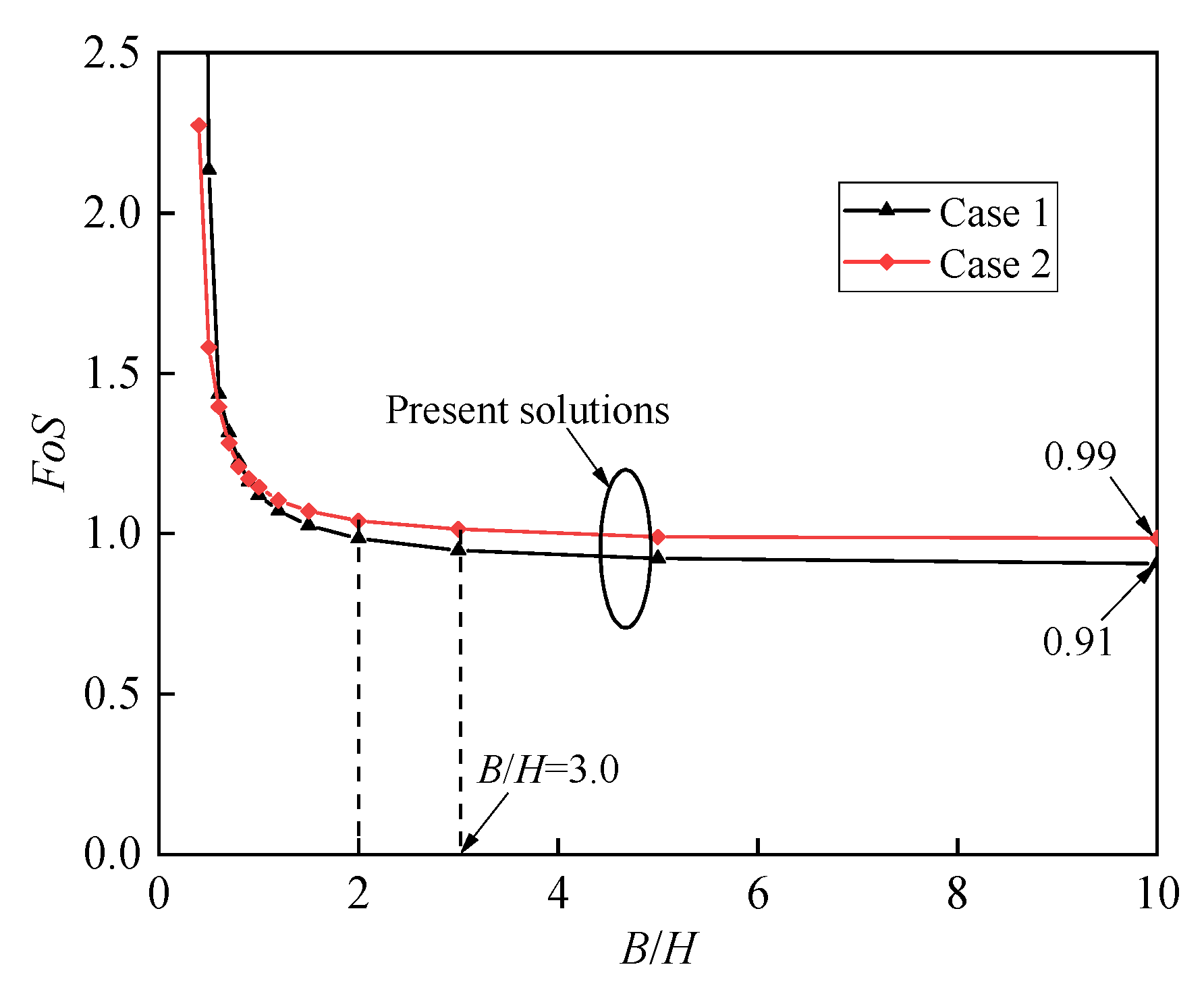
It can be seen from Table 5 that the present 3D solutions are in good agreement with the previous FoS solutions. It should be noted that the previous FoS solutions were obtained under 2D plane strain, and it is clear from Figure 10 that ratio B/H has a significant impact on FoS solutions. When the width of the failure block is greater than slope height (), FoS solutions under 2D plane strain will be adequate; however, for conditions where the width of slope is limited (), a 3D stability analysis will be more appropriate and advanced to estimate the FoS solutions of slope.
8. Conclusions
Based on the upper bound theorem of limit analysis, this study presents a chart-based stability analysis to investigate the stability of a 3D slope in disturbed rock masses following the Generalized Hoek–Brown failure criterion. Analytical expression of the FoS of 3D slope is proposed in virtue of the strength reduction technique, and a set of stability charts for slope are proposed based on the index SR = σci/γH. Modified equations to estimate the slope angle weight factor fβ_3D are proposed to build a fast and convenient method to solve the FoS of 3D slopes. A case study is conducted to apply the present stability charts on practical cases. The main conclusions of the present study can be drawn as follows:
- Validities of the present study and index SR on estimating the FoS solutions of a 3D slope in disturbed rock masses are verified that for a slope with given B/H; slope angle β; and Hoek–Brown strength parameters GSI, mi, and D, the FoS of slope is still only related to index SR.
- A parametric analysis is conducted to investigate the effects of 3D character and rock mass disturbance on slope stability. It is shown that B/H and the rock mass disturbance factor D have significant influences on slope stability and should be considered in stability analyses of slopes in rock masses.
- A series of stability charts are presented and modified equations to determine the slope angle weighting factor fβ_3D considering the 3D character of slope are presented to provide a convenient and straightforward way to estimate FoS solutions of 3D slopes in disturbed rock masses.
- A case study is conducted to apply the presented stability charts to practical cases. The results indicated that the present FoS solutions obtained using the stability charts in conjunction with the slope angle weighting factor fβ_3D are in good agreement with the analytical solutions. The validity of the present stability charts and the equations to estimate the slope angle weighting factors fβ_3D are verified.
Author Contributions
J.X., methodology, validation, formal analysis, data curation, writing—original draft, and visualization. X.W., validation, formal analysis, data curation, and writing—original draft. P.X., validation, formal analysis, data curation, writing—original draft. R.W., validation, formal analysis, data curation, and writing—original draft. D.D., writing and visualization. All authors have read and agreed to the published version of the manuscript.
Funding
This work was supported by the National Natural Science Foundation of China (52208327, 52108305), the Natural Science Foundation of Jiangsu Province (BK20210256), and the Fundamental Research Funds for the Central Universities (2242022k30030 and 2242022k30031).
Data Availability Statement
The datasets in the current study are available from the corresponding author on reasonable request. The data are not publicly available due to privacy.
Acknowledgments
The financial support is greatly appreciated.
Conflicts of Interest
The authors declare that they have no known competing financial interests or personal relationships that could have appeared to influence the work reported in this paper.
References
- Hoek, E.; Brown, E.T. Empirical strength criterion for rock masses. J. Geotech. Eng. Div. ASCE 1980, 106, 1013–1035. [Google Scholar] [CrossRef]
- Hoek, E.; Carranza-Torres, C.; Corkum, B. Hoek–Brown failure criterion-2002 edition. Proc. NARMS-Tac 2002, 1, 267–273. [Google Scholar]
- Yang, X.L. Effect of Pore-Water Pressure on 3D stability of rock slope. Int. J. Geomech. 2017, 17, 06017015. [Google Scholar] [CrossRef]
- Pan, Q.J.; Jiang, Y.J.; Dias, D. Probabilistic stability analysis of a three-dimensional rock slope characterized by the Hoek-Brown failure criterion. J. Comput. Civ. Eng. 2017, 31, 04017046. [Google Scholar] [CrossRef]
- Qin, C.B.; Chian, S.C.; Wang, C.Y. Kinematic analysis of pile behavior for improvement of slope stability in fractured and saturated Hoek-Brown rock masses. Int. J. Numer. Anal. Methods Geomech. 2017, 41, 803–827. [Google Scholar] [CrossRef]
- Li, A.J.; Merifield, R.S.; Lyamin, A.V. Stability charts for rock slopes based on the Hoek–Brown failure criterion. Int. J. Rock Mech. Min. Sci. 2008, 45, 689–700. [Google Scholar] [CrossRef]
- Li, A.J.; Lyamin, A.V.; Merifield, R.S. Seismic rock slope stability charts based on limit analysis methods. Comput. Geotech. 2009, 36, 135–148. [Google Scholar] [CrossRef]
- Xu, J.S.; Yang, X.L. Seismic stability analysis and charts of a 3D rock slope in Hoek–Brown media. Int. J. Rock Mech. Min. Sci. 2018, 112, 64–76. [Google Scholar] [CrossRef]
- Saada, Z.; Maghous, S.; Garnier, D. Stability analysis of rock slopes subjected to seepage forces using the modified Hoek–Brown criterion. Int. J. Rock Mech. Min. Sci. 2012, 55, 45–54. [Google Scholar] [CrossRef]
- Jiang, X.Y.; Cui, P.; Liu, C.Z. A chart-based seismic stability analysis method for rock slopes using Hoek–Brown failure criterion. Eng. Geol. 2016, 209, 196–208. [Google Scholar] [CrossRef]
- Shen, J.Y.; Karakus, M.; Xu, C.S. Chart–based slope stability assessment using the Generalized Hoek–Brown criterion. Int. J. Rock Mech. Min. Sci. 2013, 64, 210–219. [Google Scholar] [CrossRef]
- Sun, C.W.; Chai, J.R.; Xu, Z.G.; Qin, Y.; Chen, X.Z. Stability charts for rock mass slopes based on the Hoek–Brown strength reduction technique. Eng. Geol. 2016, 214, 94–106. [Google Scholar] [CrossRef]
- Li, A.J.; Merifield, R.S.; Lyamin, A.V. Effect of rock mass disturbance on the stability of rock slopes using the Hoek–Brown failure criterion. Comput. Geotech. 2011, 38, 546–558. [Google Scholar] [CrossRef]
- Li, A.J.; Qian, Z.G.; Jiang, J.C.; Lyamin, A. Seismic slope stability evaluation considering rock mass disturbance varying in the slope. KSCE J. Civ. Eng. 2019, 23, 1043–1054. [Google Scholar] [CrossRef]
- Park, D. Measures of slope stability in bonded soils governed by linear failure criterion with tensile strength cut-off. Comput. Geotech. 2023, 161, 105610. [Google Scholar] [CrossRef]
- Michalowski, R.L.; Park, D. Stability assessment of slopes in rock governed by the Hoek-Brown strength criterion. Int. J. Rock Mech. Min. Sci. 2020, 127, 104217. [Google Scholar] [CrossRef]
- Park, D.; Michalowski, R.L. Three-dimensional stability assessment of slopes in intact rock governed by the Hoek-Brown failure criterion. Int. J. Rock Mech. Min. Sci. 2021, 137, 104522. [Google Scholar] [CrossRef]
- Xu, J.S.; Du, X.L. Seismic stability of 3D rock slopes based on a multi-cone failure mechanism. Rock Mech. Rock Eng. 2023, 56, 1595–1605. [Google Scholar] [CrossRef]
- Hu, Y.N.; Ji, J.; Sun, Z.B.; Dias, D. First order reliability-based design optimization of 3D pile-reinforced slopes with Pareto optimality. Comput. Geotech. 2023, 162, 105635. [Google Scholar] [CrossRef]
- Sun, Z.; Zhao, Y.; Hu, Y.; Dias, D.; Ji, J. Probabilistic analysis of width-limited 3D slope in spatially variable soils: UBLA enhanced with efficiency-improved discretization of horn-like failure mechanism. Int. J. Numer. Anal. Methods Geomech. 2023, 47, 3129–3157. [Google Scholar] [CrossRef]
- Michalowski, R.L. Three-dimensional stability of slopes and excavations. Geotechnique 2009, 59, 839–850. [Google Scholar] [CrossRef]
- Gao, Y.F.; Zhang, F.; Lei, G.H.; Li, D.Y.; Wu, Y.X.; Zhang, N. Stability charts for 3D failures of homogeneous slopes. J. Geotech. Geoenviron. Eng. 2013, 139, 1528–1538. [Google Scholar] [CrossRef]
- Gao, Y.F.; Zhu, D.S.; Zhang, F.; Lei, G.H.; Qin, H.Y. Stability analysis of three-dimensional slopes under water drawdown conditions. Can. Geotech. J. 2014, 51, 1355–1364. [Google Scholar] [CrossRef]
- Pérez-Reya, I.; Alejanoa, L.R.; Riquelmeb, A.; González-deSantosa, L. Failure mechanisms and stability analyses of granitic boulders focusing a case study in Galicia (Spain). Int. J. Rock Mech. Min. Sci. 2019, 119, 58–71. [Google Scholar] [CrossRef]
- Zhang, J.H.; Wang, W.J.; Zhang, D.B.; Zhang, B.; Meng, F. Safe range of retaining pressure for three-dimensional face of pressurized tunnels based on limit analysis and reliability method. KSCE J. Civ. Eng. 2018, 22, 4645–4656. [Google Scholar] [CrossRef]
- Huang, F.; Zhao, L.H.; Ling, T.H.; Yang, X.L. Rock mass collapse mechanism of concealed karst cave beneath deep tunnel. Int. J. Rock Mech. Min. Sci. 2017, 91, 133–138. [Google Scholar] [CrossRef]
- Sonmez, H.; Ulusay, R. Modifications to the geological strength index (GSI) and their applicability to stability of slopes. Int. J. Rock Mech. Min. Sci. 1999, 36, 743–760. [Google Scholar] [CrossRef]
Figure 1.
Classification of rock masses adopted from Li et al. [6].
Figure 1.
Classification of rock masses adopted from Li et al. [6].
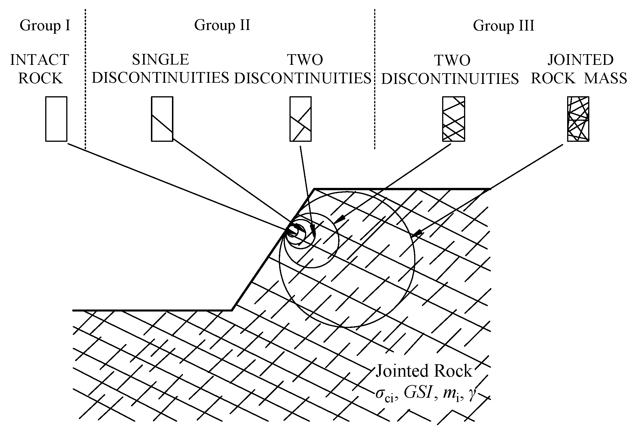
Figure 2.
Generalized Hoek–Brown failure criterion and its fitting curve from Li et al. [6].
Figure 2.
Generalized Hoek–Brown failure criterion and its fitting curve from Li et al. [6].
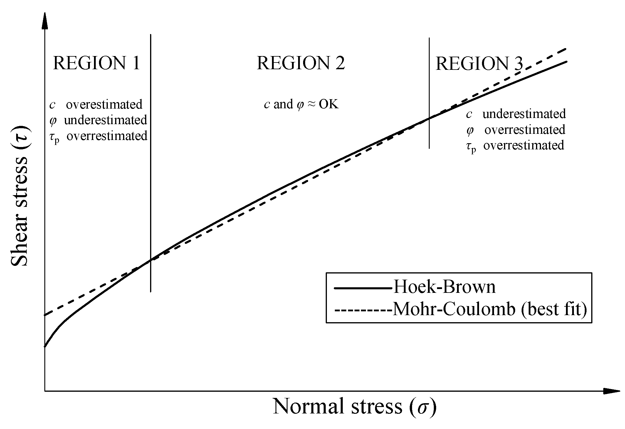
Figure 3.
Failure mechanism of slope (a) with plane insert and (b) 3D horn failure mechanism.

Figure 4.
Effects of rock mass disturbance on stability of slope in Hoek–Brown media and (a) B/H = 0~10 with different D; (b) D = 0~1.0 with different β.
Figure 4.
Effects of rock mass disturbance on stability of slope in Hoek–Brown media and (a) B/H = 0~10 with different D; (b) D = 0~1.0 with different β.
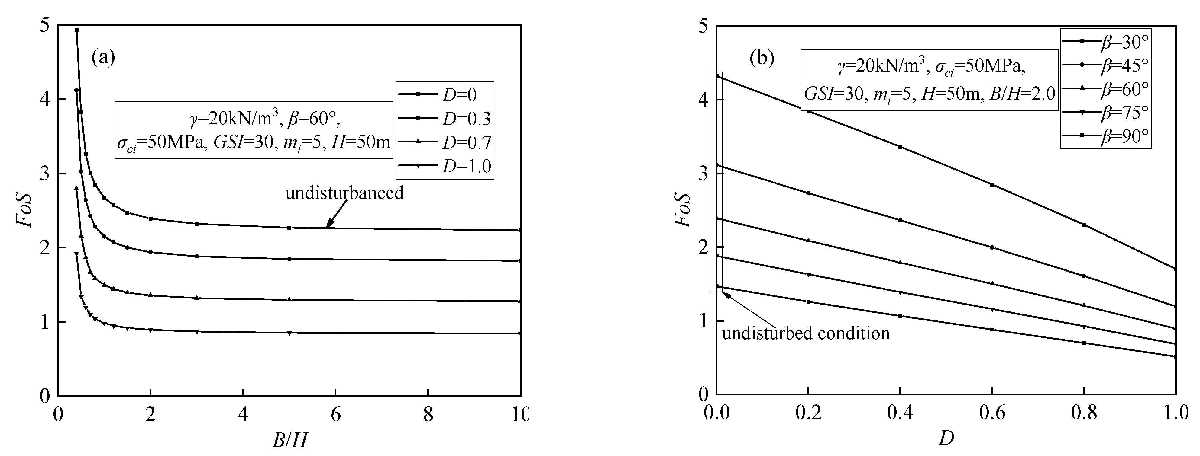
Figure 5.
Stability charts of slope in Hoek–Brown media with D = 0 (undisturbed) and (a) B/H = 0.7; (b) B/H = 1.0; (c) B/H = 1.2; (d) B/H = 1.5; (e) B/H = 2.0; (f) B/H = 5.0.
Figure 5.
Stability charts of slope in Hoek–Brown media with D = 0 (undisturbed) and (a) B/H = 0.7; (b) B/H = 1.0; (c) B/H = 1.2; (d) B/H = 1.5; (e) B/H = 2.0; (f) B/H = 5.0.
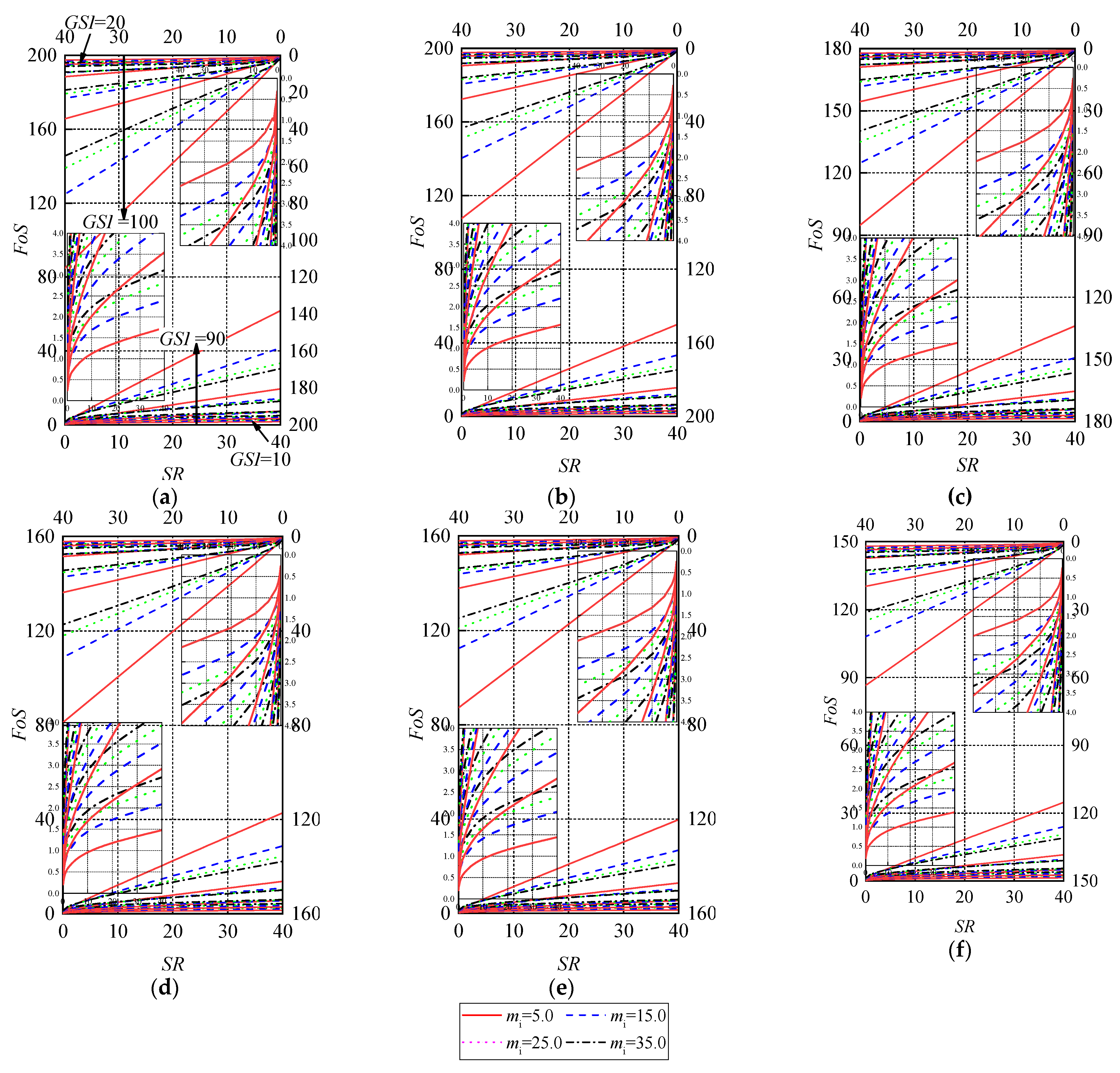
Figure 6.
Stability charts of slope in Hoek–Brown media with D = 0.3 and (a) B/H = 0.7; (b) B/H = 1.0; (c) B/H = 1.2; (d) B/H = 1.5; (e) B/H = 2.0; (f) B/H = 5.0.
Figure 6.
Stability charts of slope in Hoek–Brown media with D = 0.3 and (a) B/H = 0.7; (b) B/H = 1.0; (c) B/H = 1.2; (d) B/H = 1.5; (e) B/H = 2.0; (f) B/H = 5.0.
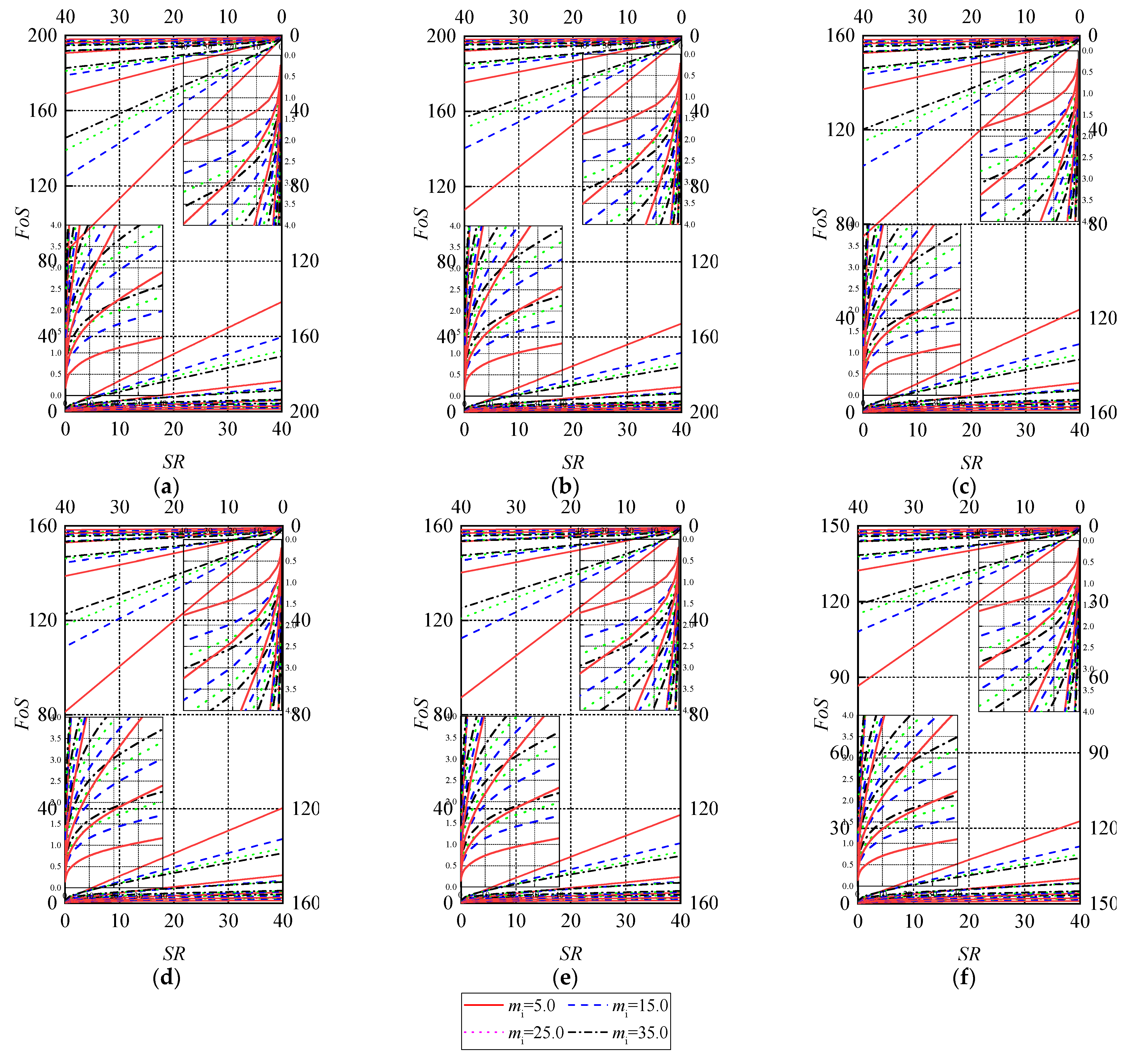
Figure 7.
Stability charts of slope in Hoek–Brown media with D = 0.7 and (a) B/H = 0.7; (b) B/H = 1.0; (c) B/H = 1.2; (d) B/H = 1.5; (e) B/H = 2.0; (f) B/H = 5.0.
Figure 7.
Stability charts of slope in Hoek–Brown media with D = 0.7 and (a) B/H = 0.7; (b) B/H = 1.0; (c) B/H = 1.2; (d) B/H = 1.5; (e) B/H = 2.0; (f) B/H = 5.0.

Figure 8.
Stability charts of slope in Hoek–Brown media with D = 1.0 and (a) B/H = 0.7; (b) B/H = 1.0; (c) B/H = 1.2; (d) B/H = 1.5; (e) B/H = 2.0; (f) B/H = 5.0.
Figure 8.
Stability charts of slope in Hoek–Brown media with D = 1.0 and (a) B/H = 0.7; (b) B/H = 1.0; (c) B/H = 1.2; (d) B/H = 1.5; (e) B/H = 2.0; (f) B/H = 5.0.
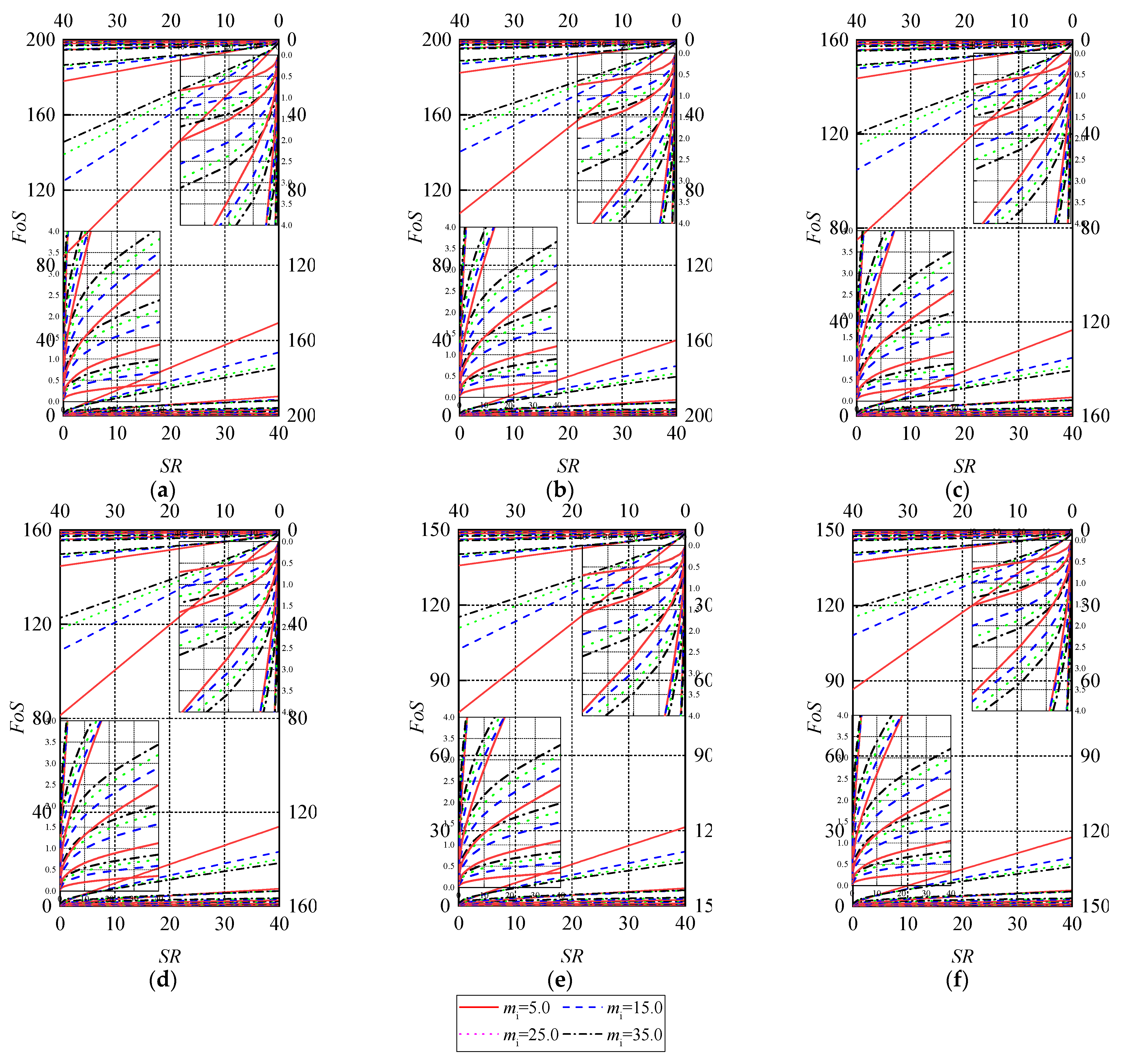
Figure 9.
Slope angle weighting factor fβ versus B/H.
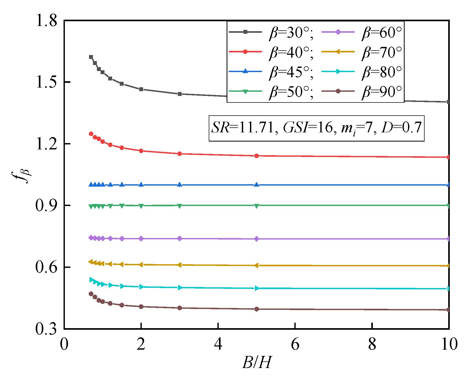
Figure 10.
FoS solution of slope from case study under 3D condition.

Table 1.
Comparison of present 3D FoS solutions with FoS solutions under 2D plane strain.
| Limit Analysis—Lower Bound | SLIDE-Limit Equilibrium Using Equivalent Mohr–Coulomb Parameters | Limit Analysis | |||||||
|---|---|---|---|---|---|---|---|---|---|
| Nonlinear HB | Equations (5)–(7) | Equations (5), (6) and (9) | Equations (5), (6) and (10) | Present 3D Solutions (B→∞) | |||||
| β/° | GSI | mi | SR | FoS0 | FoS1 | FoS2 | FoS3 | FoS4 | FoS |
| 30 | 100 | 5 | 0.070 | 1.0 | 1.014 | 0.988 | - | 1.0 | 0.9872 |
| 30 | 100 | 15 | 0.026 | 1.0 | 1.020 | 0.999 | - | 1.024 | 1.0243 |
| 30 | 100 | 25 | 0.016 | 1.0 | 1.023 | 1.003 | - | 1.036 | 1.0431 |
| 30 | 100 | 35 | 0.011 | 1.0 | 1.024 | 1.007 | - | 1.044 | 1.0327 |
| 30 | 70 | 5 | 0.218 | 1.0 | 1.018 | 0.985 | - | 1.011 | 1.0101 |
| 30 | 70 | 15 | 0.075 | 1.0 | 1.023 | 0.996 | - | 1.028 | 1.0202 |
| 30 | 70 | 25 | 0.045 | 1.0 | 1.024 | 1.004 | - | 1.035 | 1.0272 |
| 30 | 70 | 35 | 0.032 | 1.0 | 1.025 | 1.010 | - | 1.040 | 1.0306 |
| 30 | 50 | 5 | 0.461 | 1.0 | 1.020 | 0.993 | - | 1.014 | 1.0101 |
| 30 | 50 | 15 | 0.153 | 1.0 | 1.024 | 1.003 | - | 1.026 | 1.0171 |
| 30 | 50 | 25 | 0.091 | 1.0 | 1.025 | 1.024 | - | 1.032 | 1.0233 |
| 30 | 50 | 35 | 0.065 | 1.0 | 1.026 | 1.008 | - | 1.036 | 1.0302 |
| 30 | 30 | 5 | 1.057 | 1.0 | 1.022 | 1.001 | - | 1.012 | 1.0101 |
| 30 | 30 | 15 | 0.323 | 1.0 | 1.026 | 1.003 | - | 1.026 | 1.0162 |
| 30 | 30 | 25 | 0.185 | 1.0 | 1.026 | 1.005 | - | 1.031 | 1.0213 |
| 30 | 30 | 35 | 0.129 | 1.0 | 1.027 | 1.004 | - | 1.035 | 1.0278 |
| 30 | 10 | 5 | 4.363 | 1.0 | 1.023 | 1.002 | - | 1.006 | 1.0101 |
| 30 | 10 | 15 | 0.943 | 1.0 | 1.025 | 1.007 | - | 1.023 | 1.0168 |
| 30 | 10 | 25 | 0.460 | 1.0 | 1.026 | 0.996 | - | 1.033 | 1.0254 |
| 30 | 10 | 35 | 0.286 | 1.0 | 1.026 | 1.004 | - | 1.040 | 1.0316 |
| 45 | 100 | 5 | 0.135 | 1.0 | 1.000 | 1.008 | 1.022 | 1.027 | 0.9857 |
| 45 | 100 | 15 | 0.058 | 1.0 | 1.005 | 1.041 | 1.003 | 1.086 | 0.9886 |
| 45 | 100 | 25 | 0.036 | 1.0 | 1.012 | 1.047 | 1.003 | 1.110 | 0.9900 |
| 45 | 100 | 35 | 0.026 | 1.0 | 1.015 | 1.060 | 1.005 | 1.126 | 0.9900 |
| 45 | 70 | 5 | 0.469 | 1.0 | 1.001 | 1.038 | 1.001 | 1.055 | 0.9840 |
| 45 | 70 | 15 | 0.176 | 1.0 | 1.012 | 1.080 | 1.002 | 1.098 | 0.9900 |
| 45 | 70 | 25 | 0.108 | 1.0 | 1.017 | 1.060 | 1.007 | 1.113 | 0.9900 |
| 45 | 70 | 35 | 0.077 | 1.0 | 1.019 | 1.061 | 1.009 | 1.123 | 0.9900 |
| 45 | 50 | 5 | 1.046 | 1.0 | 1.004 | 1.045 | 1.001 | 1.063 | 0.9853 |
| 45 | 50 | 15 | 0.369 | 1.0 | 1.009 | 1.065 | 1.004 | 1.098 | 0.9900 |
| 45 | 50 | 25 | 0.222 | 1.0 | 1.020 | 1.066 | 1.010 | 1.110 | 0.9900 |
| 45 | 50 | 35 | 0.158 | 1.0 | 1.021 | 1.044 | 1.011 | 1.118 | 0.9900 |
| 45 | 30 | 5 | 2.593 | 1.0 | 1.011 | 1.066 | 0.999 | 1.060 | 0.9869 |
| 45 | 30 | 15 | 0.829 | 1.0 | 1.018 | 1.070 | 1.007 | 1.094 | 0.9900 |
| 45 | 30 | 25 | 0.480 | 1.0 | 1.021 | 1.074 | 1.010 | 1.110 | 0.9900 |
| 45 | 30 | 35 | 0.334 | 1.0 | 1.024 | 1.085 | 1.011 | 1.118 | 1.0101 |
| 45 | 10 | 5 | 13.585 | 1.0 | 1.014 | 1.087 | 1.000 | 1.039 | 0.9847 |
| 45 | 10 | 15 | 3.155 | 1.0 | 1.023 | 1.106 | 1.005 | 1.080 | 0.9900 |
| 45 | 10 | 25 | 1.552 | 1.0 | 1.023 | 1.107 | 1.009 | 1.103 | 0.9900 |
| 45 | 10 | 35 | 0.969 | 1.0 | 1.026 | 1.079 | 1.010 | 1.115 | 0.9900 |
| 60 | 100 | 5 | 0.232 | 1.0 | 1.001 | 1.033 | 1.043 | - | 0.9822 |
| 60 | 100 | 15 | 0.130 | 1.0 | 1.004 | 1.114 | 1.026 | - | 1.0101 |
| 60 | 100 | 25 | 0.088 | 1.0 | 1.004 | 1.146 | 1.035 | - | 1.0155 |
| 60 | 100 | 35 | 0.066 | 1.0 | 1.004 | 1.141 | 1.040 | - | 1.0241 |
| 60 | 70 | 5 | 0.946 | 1.0 | 1.013 | 1.059 | 1.024 | - | 0.9891 |
| 60 | 70 | 15 | 0.435 | 1.0 | 1.004 | 1.143 | 1.033 | - | 1.0153 |
| 60 | 70 | 25 | 0.276 | 1.0 | 1.004 | 1.161 | 1.043 | - | 1.0252 |
| 60 | 70 | 35 | 0.20 | 1.0 | 1.005 | 1.183 | 1.047 | - | 1.0284 |
| 60 | 50 | 5 | 2.337 | 1.0 | 1.005 | 1.124 | 1.026 | - | 0.9900 |
| 60 | 50 | 15 | 0.953 | 1.0 | 1.004 | 1.171 | 1.036 | - | 1.0201 |
| 60 | 50 | 25 | 0.584 | 1.0 | 1.008 | 1.176 | 1.046 | - | 1.0267 |
| 60 | 50 | 35 | 0.419 | 1.0 | 1.009 | 1.172 | 1.049 | - | 1.0302 |
| 60 | 30 | 5 | 6.439 | 1.0 | 1.009 | 1.150 | 1.023 | - | 1.0101 |
| 60 | 30 | 15 | 2.317 | 1.0 | 1.009 | 1.197 | 1.044 | - | 1.0239 |
| 60 | 30 | 25 | 1.356 | 1.0 | 1.010 | 1.201 | 1.049 | - | 1.0294 |
| 60 | 30 | 35 | 0.945 | 1.0 | 1.011 | 1.230 | 1.051 | - | 1.0319 |
| 60 | 10 | 5 | 38.926 | 1.0 | 1.004 | 1.183 | 1.013 | - | 0.9900 |
| 60 | 10 | 15 | 11.734 | 1.0 | 1.013 | 1.257 | 1.048 | - | 1.0288 |
| 60 | 10 | 25 | 5.928 | 1.0 | 1.017 | 1.261 | 1.054 | - | 1.0366 |
| 60 | 10 | 35 | 3.729 | 1.0 | 1.018 | 1.258 | 1.059 | - | 1.0403 |
| Input Parameters | Case 1 | Case 2 | Case 3 |
|---|---|---|---|
| GSI | 30 | 30 | 30 |
| mi | 8 | 8 | 8 |
| β/° | 60 | 60 | 60 |
| σci/kPa | 20 | 25 | 250 |
| γ/(kN/m3) | 23 | 28.75 | 23.96 |
| H/m | 25 | 25 | 300 |
| SR (σci/γH) | 34.783 | 34.783 | 34.783 |
| FoS (D = 0) | |||
| Bishop simplified | 2.026 | 2.026 | 2.026 |
| Janbu simplified | 1.934 | 1.934 | 1.934 |
| Spencer | 2.032 | 2.032 | 2.032 |
| Morgenstern–Price | 2.027 | 2.027 | 2.027 |
| Phase2 8.0 (FEM) | 2.000 | 2.040 | 2.030 |
| Present 3D solution (B→∞) | |||
| D = 0 | 2.0230 | 2.0230 | 2.0229 |
| D = 0.3 | 1.7066 | 1.7066 | 1.7066 |
| D = 0.7 | 1.2477 | 1.2477 | 1.2477 |
| D = 1.0 | 0.8416 | 0.8416 | 0.8416 |
| H/m | β/° | γ/ (kN/m3) | σci/ kPa | GSI | mi | D | fβ | ||||
|---|---|---|---|---|---|---|---|---|---|---|---|
| Shen et al. [11] | Sun et al. [12] | Present solution | |||||||||
| B/H =0.7 | B/H =1.0 | B/H →∞ | |||||||||
| 184 | 55 | 27 | 153 | 47 | 9 | 0.9 | 0.793 | 0.817 | 0.825 | 0.827 | 0.828 |
| 140 | 34 | 26 | 50 | 28 | 8 | 0.7 | 1.259 | 1.264 | 1.439 | 1.389 | 1.290 |
| 220 | 45 | 27 | 65 | 44 | 17 | 0.8 | 1.000 | 1.000 | 1.000 | 1.000 | 1.000 |
| 135 | 65 | 27 | 172 | 58 | 9 | 0.9 | 0.637 | 0.753 | 0.734 | 0.732 | 0.733 |
| 70 | 50 | 27 | 29 | 41 | 7 | 0.8 | 0.885 | 0.901 | 0.905 | 0.903 | 0.905 |
| 110 | 45 | 26.5 | 50 | 25 | 10 | 0.7 | 1.000 | 1.000 | 1.000 | 1.000 | 1.000 |
| 270 | 45 | 27 | 109 | 39 | 18 | 0.9 | 1.000 | 1.000 | 1.000 | 1.000 | 1.000 |
| 170 | 55 | 30 | 104 | 48 | 7 | 0.7 | 0.793 | 0.814 | 0.830 | 0.828 | 0.831 |
| 60 | 60 | 27 | 65 | 44 | 13 | 1.0 | 0.711 | 0.710 | 0.754 | 0.752 | 0.751 |
| 35 | 67 | 27 | 109 | 28 | 12 | 1.0 | 0.609 | 0.571 | 0.664 | 0.659 | 0.651 |
| 63 | 35 | 27 | 109 | 28 | 12 | 1.0 | 1.232 | 1.252 | 1.361 | 1.326 | 1.256 |
| 70 | 49 | 27 | 3 | 49 | 25 | 1.0 | 0.905 | 0.941 | 0.921 | 0.920 | 0.922 |
| 58 | 50 | 27 | 5 | 55 | 22 | 1.0 | 0.885 | 0.922 | 0.900 | 0.902 | 0.904 |
| 60 | 48 | 27 | 5 | 54 | 22 | 1.0 | 0.925 | 0.944 | 0.937 | 0.939 | 0.940 |
| 60 | 52 | 27 | 5 | 56 | 22 | 1.0 | 0.847 | 0.930 | 0.865 | 0.868 | 0.869 |
| 40 | 71 | 27 | 50 | 33 | 14 | 1.0 | 0.558 | 0.538 | 0.621 | 0.614 | 0.602 |
| 110 | 50 | 27 | 50 | 25 | 14 | 1.0 | 0.885 | 0.903 | 0.899 | 0.900 | 0.901 |
| 41 | 50 | 27 | 3 | 46 | 24 | 1.0 | 0.885 | 0.899 | 0.900 | 0.902 | 0.904 |
| 41 | 55 | 27 | 3 | 49 | 24 | 1.0 | 0.793 | 0.848 | 0.820 | 0.819 | 0.820 |
| 46 | 55 | 27 | 3 | 50 | 24 | 1.0 | 0.793 | 0.810 | 0.820 | 0.819 | 0.821 |
| 57 | 49 | 27 | 3 | 48 | 24 | 1.0 | 0.905 | 0.909 | 0.921 | 0.921 | 0.922 |
| 57 | 37 | 27 | 3 | 48 | 24 | 1.0 | 1.179 | 1.185 | 1.374 | 1.328 | 1.221 |
| 57 | 40 | 27 | 3 | 48 | 24 | 1.0 | 1.103 | 1.130 | 1.288 | 1.246 | 1.154 |
| 57 | 42 | 27 | 3 | 48 | 24 | 1.0 | 1.056 | 1.083 | 1.235 | 1.198 | 1.113 |
| 27 | 45 | 25 | 0.75 | 100 | 10 | 0 | 1.000 | 1.000 | 1.000 | 1.000 | 1.000 |
| 50 | 60 | 23 | 10 | 30 | 8 | 1.0 | 0.711 | 0.722 | 0.746 | 0.746 | 0.745 |
| 50 | 45 | 27 | 13.5 | 30 | 5 | 0.7 | 1.000 | 1.000 | 1.000 | 1.000 | 1.000 |
| 25 | 45 | 27 | 5.4 | 20 | 20 | 0.7 | 1.000 | 1.000 | 1.000 | 1.000 | 1.000 |
| 5 | 30 | 27 | 2.7 | 10 | 5 | 0.5 | 1.375 | 1.438 | 1.615 | 1.551 | 1.433 |
| 25 | 75 | 25 | 0.625 | 80 | 15 | 0.3 | 0.511 | 0.525 | 0.605 | 0.591 | 0.577 |
| 250 | 60 | 23 | 46 | 50 | 35 | 1.0 | 0.711 | 0.652 | 0.746 | 0.745 | 0.743 |
Table 4.
Modified equations to estimate the slope angle weighting factor fβ_3D of 3D slope (0≤ FoS ≤4).
Table 4.
Modified equations to estimate the slope angle weighting factor fβ_3D of 3D slope (0≤ FoS ≤4).
| B/H | Regression Equations—fβ_B/H | Fitting Degree—R2 |
|---|---|---|
| 0.7 | 35.7 β−0.9091, 30° ≤ β < 45° | 0.9992 |
| 62.2 β−1.082, 45° < β ≤ 90° | 0.9995 | |
| 1.0 | 28.52 β−0.8569, 30° ≤ β < 45° | 0.9997 |
| 2.26 e−0.01849β, 45° < β ≤ 90° | 0.9993 | |
| 1.2 | 26.04 β−0.8355, 30° ≤ β < 45° | 0.9998 |
| 2.301 e−0.01882β, 45° < β ≤ 90° | 0.9996 | |
| 1.5 | 23.91 β−0.816, 30° ≤ β < 45° | 0.9994 |
| 2.342 e−0.01914β, 45° < β ≤ 90° | 0.9998 | |
| 2.0 | 22.38 β−0.8012, 30° ≤ β < 45° | 0.9998 |
| 2.382 e−0.01945β, 45° < β ≤ 90° | 0.9998 | |
| 5.0 | 19.85 β−0.7745, 30° ≤ β < 45° | 0.9999 |
| 2.442 e−0.01994β, 45° < β ≤ 90° | 0.9996 |
Table 5.
FoS solutions of slopes from case study.
| Input Parameters | Case 1 | Case 2 | |
|---|---|---|---|
| β/° | 34 | 60 | |
| GSI | 16 | 37 | |
| mi | 7 | 9.04 | |
| D | 0.7 | 1.0 | |
| σci/MPa | 5.2 | 40 | |
| γ/(kN/m3) | 22.2 | 21 | |
| H/m | 20 | 80 | |
| SR | 11.71 | 23.81 | |
| FoS | Li et al. [6] | 0.90 | 1.13 |
| Shen et al. [11] | 0.95 | 1.22 | |
| Sun et al. [12] | 0.93 | 1.06 | |
| ABAQUS by Sun et al. [12] | 0.97 | 1.14 | |
| Present 3D solutions | B/H = 5.0 from present charts | 0.92 | 0.99 |
| B/H→∞ | 0.89 | 0.98 |
Disclaimer/Publisher’s Note: The statements, opinions and data contained in all publications are solely those of the individual author(s) and contributor(s) and not of MDPI and/or the editor(s). MDPI and/or the editor(s) disclaim responsibility for any injury to people or property resulting from any ideas, methods, instructions or products referred to in the content. |
© 2023 by the authors. Licensee MDPI, Basel, Switzerland. This article is an open access article distributed under the terms and conditions of the Creative Commons Attribution (CC BY) license (https://creativecommons.org/licenses/by/4.0/).
Share and Cite
MDPI and ACS Style
Xu, J.; Wang, X.; Xie, P.; Wang, R.; Du, D. Effect of Rock Mass Disturbance on Stability of 3D Hoek–Brown Slope and Charts. Buildings 2024, 14, 114. https://doi.org/10.3390/buildings14010114
AMA Style
Xu J, Wang X, Xie P, Wang R, Du D. Effect of Rock Mass Disturbance on Stability of 3D Hoek–Brown Slope and Charts. Buildings. 2024; 14(1):114. https://doi.org/10.3390/buildings14010114
Chicago/Turabian StyleXu, Jingshu, Xinrui Wang, Pengfei Xie, Ruotong Wang, and Dianchun Du. 2024. "Effect of Rock Mass Disturbance on Stability of 3D Hoek–Brown Slope and Charts" Buildings 14, no. 1: 114. https://doi.org/10.3390/buildings14010114
Note that from the first issue of 2016, this journal uses article numbers instead of page numbers. See further details here.