

Influence of the Uplifting Mechanism of Embedded Footings on the Nonlinear Static Response of Steel Concentrically Braced Frames

Department of Strength of Materials and Structural Engineering, Polytechnic University of Catalonia (UPC), 08222 Barcelona, Spain
*
Author to whom correspondence should be addressed.
Buildings 2024, 14(4), 1145; https://doi.org/10.3390/buildings14041145
Submission received: 5 March 2024
/
Revised: 26 March 2024
/
Accepted: 15 April 2024
/
Published: 18 April 2024
(This article belongs to the Special Issue Application of Soil-Structure Interaction in Construction)
Abstract
:The aim of this paper is to evaluate the nonlinear static response of steel concentrically braced frames (CBFs) by considering the response of embedded footings in granular soils using the Beam on Nonlinear Winkler Foundation (BNWF) approach. To model the vertical stress-displacement behaviour of footings, it is possible to define a backbone curve capable of reproducing the total response by adding in series the behaviour of the compression zone with that of the tension zone. When uplift of the soil–foundation system is allowed, it has been demonstrated that it is necessary to consider the horizontal stresses of the native soil on site and the degree of compaction of the soil mass above the footing to avoid significant deviations between the analysis results and the real response. The tension zone in the backbone curves was calibrated while considering these parameters, and given the difficulty associated with their calibration, an estimation is reported that could also be used in the case of practical applications. The implementation of the model has been validated through various pushover analyses on an archetype steel CBF originally tested on a fixed base condition, and predictions were made for the flexible base condition, considering different types of soil and different embedment depths. The results suggest that there is a relationship between the nonlinear static response of steel CBF structures and the uplift mechanism of embedded footings that is influenced by the embedment depth of the footings and the shape of the tension-displacement zone of the backbone curves considered in the modelling process. The proposed model can be used to simulate the flexible base condition of CBF structures on embedded footings using nonlinear springs when carrying out performance-based design procedures.
1. Introduction
Current structural design codes [1,2,3] require nonlinear static analyses to be performed for new and existing structural systems when a seismic performance assessment is required by the project. This requires the nonlinear response of the superstructure and infrastructure members to be included in the analytical model to account for the change in stiffness during the load application process. However, soil–structure interaction (SSI) phenomena and foundation flexibility are typically not considered when evaluating the collapse capacity of structural systems [4].
The ASCE7-16 code [5] provides formal procedures for considering soil–structure interaction phenomena in buildings; however, when applying these procedures, restrictions are considered on the design forces estimated from analyses with evidence of SSI phenomena, depending on the available ductility of the structure. The reason for this is based on the fact that, according to FEMA P-2091 [6], SSI investigations have mainly been focused on superstructure models with linear elastic behaviour. Therefore, a more in-depth study is needed to validate such limitations in terms of the relationship between superstructure nonlinearity and soil–structure interaction effects.
Steel concentrically braced frames (CBFs) are a type of structure capable of resisting lateral loads by means of a vertical truss system, in which the axes of the members are concentrically aligned with the joints. CBFs are considered efficient in resisting lateral loads due to their high lateral strength and stiffness, making them a common type of structure in seismic areas [7]. Special concentrically braced frames (SCBFs) are a special type of CBF that are dimensioned and detailed in order to maximise the inelastic drift capacity [7,8]. Earthquake-induced deformation causes buckling of the compressed braces and subsequent yielding of the tensioned braces.
The AISC 341-16 code [8] states that the maximum force transferred to the bracing connection and beam–column connection for SCBF type systems can be determined by three methods: (a) a non-linear static (pushover) analysis to determine the forces acting on the connection when the maximum capacity of the element is reached, (b) estimating the force that can be resisted before the uplift of a footing is developed, or (c) a nonlinear time-history analysis. However, the same code indicates that it is not common practice on projects for the maximum design force to be determined by any of these three methods. Therefore, the design philosophy for this type of structural system is to provide the connection with sufficient capacity to ensure the yielding of the bracing [8]. The latter is achieved by ensuring that the foundation design is capable of fully developing the resistance of the bracing [7].
Concentrically braced systems have significant overstrength that is not accounted for in current foundation design practice, which can lead to uplift of footings below the braced members and produce a “rocking” mechanism [4]. Sabelli et al. [7] note that foundation uplift can significantly attenuate the dynamic response from seismic excitation; however, the design requirements to control this uplift and the consequences of this uplift differ greatly from commonly applied design considerations for SCBF systems. They conclude by highlighting that relying on the uplift condition without taking into account a wide range of aspects required to control uplift appears to be unwise for new construction. On the other hand, several authors have reported the benefits of foundation uplift mechanisms [9,10,11,12].
In order to better understand the influence of foundation flexibility on CBF systems, Uriz and Mahin [13] developed a set of performance-based earthquake engineering analyses on a group of 3 and 6 level special concentrically braced frames (SCBFs) and buckling restrained braced frames (BRBFs) (as described in Sabelli [14]). As part of these analyses, the uplift condition was considered, and the rocking effect was evidenced in a group of models. One conclusion of this study is that the rocking effect may reduce damage to the bracing system, but not to structural and non-structural elements located elsewhere in the building [13].
Another study that reports the importance of considering foundation flexibility in the nonlinear response of the structure is provided in FEMA P-2139-4 [4] in which a “Study of One-to-Four Story Steel Special Concentrically Braced Frame” is developed to evaluate the collapse performance of low-period structures. The results of this study indicate that, when using nonlinear models to evaluate the collapse potential of SCBF steel systems, such models must include foundation flexibility and soil behaviour using nonlinear springs and dampers, as required, to allow for foundation movement and deformation, taking into account the uplift and rocking of the braced structural system. In this study, the SSI effects are considered, allowing for the full uplift condition (tension capacity equal to zero) on the buildings to be studied.
In order to demonstrate SSI phenomena, several authors [15,16,17,18] have developed procedures to model the nonlinear response of flexible foundations based on the BNWF (Beam on Nonlinear Winkler Foundation) approach. This model essentially consists of defining a bed of non-symmetric backbone curves that allow a compressive stress-displacement response to be coupled with a tensile stress-displacement response of the foundation. In addition, the model allows the moment–rotation behaviour to be reproduced by placing stiffer vertical springs in the extreme regions of the foundation that are calibrated to reproduce the vertical and rotational elastic stiffness [18].
In order to reproduce the nonlinear compressive response in shallow foundations, the procedure proposed by Raychowdhury [15] stands out, in which the material “QzSimple1”, included in the finite element-based platform Opensees [19], has been calibrated and adapted to the case of footings. This model is derived from the material originally developed by Boulanger et al. [20] and subsequently implemented in Opensees by Boulanger [21] to characterise the stress-displacement response at the pile tip. To model the compressive response, the elastic response zone, whose slope reproduces the dynamic stiffness of rigid foundations, is coupled with the nonlinear response zone calibrated by experimental data. On the other hand, Briaud and Gibbens [22] developed a set of compressive load tests on five square footings ranging in size from 1.0 m to 3.0 m. These footings were subjected to a compression load up to a penetration of 150 mm and the load-settlement curve was recorded for all footings. The results of these tests have allowed the calibration of the constitutive parameters that model the compression response zone of the footing to reproduce the expected load-settlement response for footings supported on sand.
To estimate the maximum tensile capacity of the footing, some authors [15,16,18] have proposed to set this value in their model as a percentage of the compressive bearing capacity (qu) of the footing, between 0% and 10%, and to consider a tensile response mechanism in which the constitutive parameters of the model are derived from the compressive response mechanism. In addition, FEMA P-2006 [23] presents a calculation example in which the footing uplift capacity is estimated from the footing self-weight, the weight of the soil above the footing, and the weight of the surface slab acting on the plan projection of the footing. In this case, the maximum uplift capacity is reached by considering a linear stress-displacement variation equal to the slope of the initial region of the curve modelling the compressive response. On the other hand, Raychowdhury [15] indicates that among the parameters required to apply the BNWF model, the vertical tensile capacity and the angle of internal friction of the soil have the most significant effects on the capabilities of the BNWF model to capture the force and displacement demands.
In the field of building structure design, it is common for structural engineers not to consider detailed procedures for modelling the tension behaviour of footings beyond the classical methods [24,25,26], which allow only the determination of the ultimate tension capacity of footings and which, from a practical point of view, are considered simplified and empirical, so that such traditional methods can be applied for a certain range of conditions, but all have important limitations in their application [27].
In many regions, the common practice of footing construction is characterised by shallow depths of no more than 1.0 metre. In such cases, it is evident that the uplift capacity is expected to be reduced. However, for those cases where geotechnical requirements require footings to be embedded, the influence that the stress-displacement mechanisms of such footings may have on the seismic performance assessment of CBF structures has not yet been reported, leading to a gap between analytical prediction methods and the observed collapse mechanisms when this type of structural configuration is subjected to seismic forces. However, foundation uplift is a well-known problem in the field of electrical power distribution and telecommunication towers, where the footing uplift capacity is regularly the controlling geotechnical design condition for transmission line structures [27]. Although the two areas are apparently considered to be different, the uplift issue has many similarities in both scenarios. Kulhawy et al. [28] developed a scaled experimental test programme as part of a research programme aimed at developing rational design procedures for lattice transmission line towers. The study evaluated the influence of geometric variables, the construction method, and the characteristics of the backfill above the footing on the uplift mechanism of footings embedded in granular soils. It was found that the lateral resistance of footings depends on the type of backfill material used, the degree of compaction of the backfill, and the density state of the native soil, which tends to modify the capacity, displacements, and stiffness of the soil–foundation system.
The scope of this research is focused on unifying the compression and tension response mechanisms of footings, both of which have been experimentally validated separately by means of a single model that allows such response mechanisms to be reproduced simultaneously. This model allows a more accurate assessment of the influence of the uplift mechanism of footings embedded in granular soils on the nonlinear static response of CBFs when considering soil–structure interaction phenomena. The response mechanism of embedded footings has been modelled using the BNWF approach by considering a bed of backbone curves that allow the modelling of the tension and compression response simultaneously. The proposed backbone curve was developed by coupling a curve that reproduces the tension response with the compression response curve proposed by Raychowdhury [15]. The tension zone has been constructed from a more complete model that takes into consideration the stress state of the native soil and the backfill, as well as the construction procedure of the footing, and has been experimentally validated by Kulhawy et al. [28].
Since a better description of the tension response mechanism of shallow foundations has not been considered in depth, most practitioners typically consider some simplifications to model the uplift mechanism of footings, which may lead to significant deviations from the expected structural response when performing nonlinear analyses of structures. The suggested approach in this study is viewed as an enhancement of the current methods used in practice to model the nonlinear response of footings. The simultaneous combination of an experimentally validated response in both tension and compression into a unique curve is an alternative to close the existing gap between the expected results and the real structural response when the SSI phenomena are required for conducting performance-based design procedures.
The paper is organised as follows: Section 2 describes the models used to reproduce the compression and tension response mechanisms used in the construction of the backbone curves. Section 3 presents an organised procedure for implementing the BNWF model on footings to model the nonlinear response mechanisms of the soil–foundation system. Section 4 describes the procedure for developing the fixed and flexible base models and the backbone curves used in the simulations. The following results are reported and discussed in Section 5: the relationship between the ultimate tension capacity (quT) and the ultimate compression capacity (qu) of the footings as a function of soil type and embedment depth, the relationship between the embedment depth of the footings and the nonlinear static response of steel CBF systems, the analysis of the development of the yielding mechanism of the brace in compression as a function of the embedment depth of footings, the effect of the shape of the tension curve of footings on the nonlinear response of steel CBF systems, and the variation of the ductility of the structure when the uplift mechanism of the footings is taken into consideration. Finally, the conclusions are presented in Section 6.
2. Description of the Nonlinear Response Mechanisms of Footings Considered in Flexible Base Models
2.1. BNWF (Beam on Nonlinear Winkler Foundation) Approach to Model the Compression and Tension Response Mechanisms of Footings
A more realistic backbone curve is proposed to be used in conjunction with the BNWF approach to model the nonlinear flexible base condition, given the importance of properly accounting for the foundation uplift mechanism in the global response of steel CBF structures. This model allows the compression and tension responses of the footing to be considered via the use of backbone curves distributed along the footing. To evaluate the compression response, the model proposed by Raychowdhury [15] is considered, which has been validated in the present investigation on the basis of experimental results reported by Briaud and Gibbens [29]. The response of the tension zone is reproduced from the model proposed and validated experimentally by Kulhawy et al. [28], which was originally developed to address the lack of more accurate methods for modelling the tension response of embedded lattice transmission tower foundations and is covered by the Standard IEEE 691 [27]. Therefore, a contribution of this paper is the adaptation of this knowledge to that of the steel CBF design. A schematic representation of the model considered in this research is shown in Figure 1, which consists of a steel concentrically braced frame structure supported on embedded footings with a defined embedment depth (Df).
The backbone curves are distributed under the footing in such a way that their spacing and intensity simultaneously reproduce the total vertical and rotational stiffness of the footing.
2.2. Modelling of the Total Vertical Response (Backbone Curve)
Each nonlinear spring considered in the model is obtained by combining the compression and tension responses through a backbone curve, where both response mechanisms are analysed independently (Figure 2). The proposed backbone curve is capable of reproducing the nonlinear response of embedded footings, taking into consideration the properties of the native soil, the embedment depth, and the characteristics of the backfill above the footing in the uplift mechanism. This model is proposed to be used when a nonlinear analysis of the structure on a flexible base condition is required. In Figure 2, the blue line represents the backbone curve, and the red lines show the initial stiffness for both responses. It is worth noting that the slope of the initial stiffness is not necessarily the same for both responses, as the tension behaviour is analysed independently of the compression behaviour.
2.3. Vertical Response in Compression
The vertical response in compression is modelled by a curve that has an initial elastic portion and then progressively develops a zone of inelastic behaviour (Figure 2). The main parameters that are considered to reproduce the vertical stress-displacement curve of the springs under compression loads are described below.
In the elastic portion, the behaviour is described by Equation (1):
and the range of the elastic portion is defined by Equation (2):
In the nonlinear (post-yield) portion, the curve is described by Equation (3):
where q is the instantaneous compression load, kin is the initial elastic stiffness estimated according to equations proposed by Gazetas [30], z is the instantaneous vertical displacement in compression, qo is the load at yield point, Cr is a parameter for controlling the range of the elastic portion, qu is the ultimate compression load of the soil–foundation system, z50 is the displacement at which 50% of the ultimate load is mobilised, z0 is the displacement at the yield point, and c and n are constitutive parameters controlling the shape of the nonlinear portion of the curve. The superscript (p) in the variables and denotes the plastic load cycle, according to the original model described by Boulanger et al. [20]. In order to calibrate the constitutive parameters Cr, n and c required by Equations (2) and (3), the experimental results obtained by Briaud and Gibbens [29] have been used, in which the load-settlement curve of 5 footings supported on a sandy soil subjected to a compression load application process is reported. In these tests, a sustained compressive load was applied up to a maximum deformation value of 150 mm, and the load-settlement curve was recorded for all foundations. Vertical deformations were measured using telltales at depths of 0.5 B, 1.0 B, and 2.0 B, where B is the width of the footings, and horizontal deformations were measured using inclinometers located at various distances from the edges of the foundation. The characteristics of the tested footings included in the calibration process are shown in Table 1. In this table, reference is made to the “North” and “South” locations for the 3.0 m × 3.0 m footing because according to [29], two footings of this size were tested in two different locations, one to the North and one to the South of the test site.
From a geotechnical point of view, the upper soil layers (up to a depth of 11 m) consist of a medium to dense silty sand. Given that the maximum plan dimension tested was 3.0 m, it is considered that the response of the foundations is mainly influenced by this sandy soil. Details of the field and laboratory test results and the geotechnical characteristics of the site are reported in [29].
The compression response curve of the footing has an initial elastic response zone and a nonlinear response zone. The size of the elastic response zone is given by the coefficient Cr in Equation (2) and can be estimated from the vertical static stiffness of the footing Kz according to the equations from Gazetas [30] or Pais and Kausel [31]. The nonlinear response zone must be calibrated according to the constitutive parameters n and c. However, the values of the vertical static stiffness Kz and the rotational stiffness Kyy depend on the magnitude of the soil shear modulus G, which must be estimated according to the associated shear strain level. The procedure typically used in practice consists in applying a reduction coefficient to the value of the shear modulus of stiffness associated with small deformations Gmax, which can be deduced from the propagation velocity of the transverse seismic waves Vs by means of common geophysical methods (cross-hole, down-hole, CPTU seismic, and spectral analysis of surface waves), or by means of certain laboratory tests capable of estimating parameters at small deformations (i.e., resonant column) that are frequently used in soil dynamics [32]. Thus, this value of the dynamic stiffness associated with small deformations Gmax is estimated from ρVs², where Vs is the shear wave velocity and ρ is the soil mass density estimated as the ratio of the unit weight of soil to the acceleration of gravity [33].
In the calibration process, all tested footings were analysed with the dimensions given in Table 1. The footings were considered as rigid elements with respect to the supporting soil; therefore, for the purpose of calibrating the constitutive parameters Cr, n and c, the load-settlement response of the footing was modelled by means of a single spring that reproduces the total vertical stiffness of the footing in compression. A shear wave velocity of approximately 270 m/s, estimated from cross-hole tests, was considered, from which a value of Gmax of 114.9 MPa was obtained. An angle of internal friction ϕ of 32° and a unit weight of 15.5 kN/m³ were considered, which corresponded to the average values reported in the tests. A Poisson’s ratio of 0.25 estimated according to [34] was used. The ultimate bearing capacity qu value reported in the test is associated with a settlement of 150 mm.
In order to determine the reduction coefficient of Gmax that best reproduced the compression response of the tested footings, the value of Cr was first estimated by trial and error. The vertical stiffness Kz was estimated as Cr.qu/s, where qu is the bearing capacity reported in the test and s is the settlement for the stress corresponding to Cr.qu. The iteration process was initiated from the calibration values reported by [15]. The calibration process yielded that a value of Cr = 0.3 was adequate to set the width of the elastic response zone of the footing. The coefficient G/Gmax was then estimated to ensure that the difference between the initial elastic stiffness value reported in the test and that one estimated using the equations of Gazetas [30] was less than 5% (Table 2).
Since it is common in practice to estimate the static stiffness values using the equations of Gazetas [30] or Pais and Kausel [31], the calculation using both approaches is also reported in Table 2, noting that the difference between the results obtained using both equations represents a variation of no more than 3.5%. Therefore, it is considered appropriate to estimate the initial portion of the compression response curve using either of these two approaches.
A practical way of estimating the shear modulus G associated with a given level of shear strain is by using the guidelines given in IEC 61400-6 [35] or using the reference curves published by several authors [36,37,38,39], which report the variation of G/Gmax as a function of shear strain for different types of soil. The procedure is to estimate the value of G/Gmax according to the magnitude of shear strain developed below the footing. According to [29], the value of 2B is considered a reasonable depth of influence to estimate the average strain under the footing as s/2B, where s is the magnitude of settlement and B is the footing width. From these strain values, the G/Gmax ratio can be estimated using the reference curve best suited to the geotechnical conditions of the site.
After calibrating the zone of elastic response according to the above procedure, the c value is estimated by trial and error from the range 9.29 ± 2.74 recommended by [15] to determine the value that best reproduces the response of the inelastic zone for the footings tested. It is reported that, when compared with the curves reported by Briaud and Gibbens [29], the values of c and n that best reproduce the expected response of this group of tested footings are 12.30 and 5.50, respectively. It is worth mentioning that the constitutive parameters that best matched the observed behaviour of this group of tested footings correspond to the values recommended by Vijaivergiya [40], originally calibrated to model the behaviour of q-z material for the case of piles in sand. Raychowdhury [15] highlights the closeness between the maximum estimated value considering the maximum standard deviation c = 12.03 with respect to the calibrated value for piles in sand c = 12.30. A summary of the final calibrated values of the constitutive parameters used in the simulations reported in this paper is shown in Table 3.
2.4. Vertical Response in Tension
In order to take into account the construction process of embedded footings and the stress state developed in both the backfill and the native soil, it is proposed to model the tension zone of vertical springs using the stress-displacement mechanism reported by [28] for shallow foundations subjected to uplift.
The tension side of the curve is modelled by a normalised hyperbolic curve according to Equation (4).
where the ultimate uplift capacity of the foundation quT can be estimated by Equation (5) [41]:
In Equations (4) and (5), qt is the instantaneous load in tension, zt is the instantaneous displacement in tension, Df is the embedment depth, W is the weight of the foundation Wf plus that of the soil above the embedment depth Ws, estimated as the product of the effective unit weight of the backfill and the volume it occupies, and qsu is the side resistance developed in n layers of thickness d. This resistance is mobilised along the shear surface and is a function of the stress acting on the soil and the geometry of the foundation.
For drained conditions, qsu is given by Equation (6):
where B and L are the width and length of the footing, respectively; σv’n is the effective vertical stress γ’z evaluated at the centre of each soil layer, where γ’ is the effective soil unit weight; and Kn is the estimated horizontal operating stress ratio at the centre of each soil layer, calculated as the product of the horizontal stress ratio of the soil in place Ko and a modifier that considers the construction process K/Ko where typically an excavation is made on site, the footing and pedestal are constructed, and then the backfill material is placed. δ is the friction angle of the interface of each soil layer that could be considered as δ = ϕ’ for the soil–soil interface; ϕ’ is the effective angle of internal friction of the soil; and qtu is the tip resistance that is developed from a suction mechanism at the bottom of the foundation, but is not expected to occur to any great extent under drained conditions [28].
The term σv’n K tanδ is equal to the shear stress τ(z) at a given depth z and must be evaluated separately for the native soil and for the backfill, so that the lower of the two dominates the behaviour and is used for the design. The values of K, γ’, and ϕ’ therefore correspond to the properties of the weakest soil between the native soil and the backfill.
In some cases, the backfill is the same as the soil on site, and in other cases, depending on the project specifications, it may be replaced by a material with suitable granulometric and plastic properties. In both situations, it is common practice to compact the soil at the level of the excavation and the backfill within the pit using light compaction equipment before constructing the footing, as can be seen in Figure 3a,b. In Figure 3c, the expected densification mechanism of the backfill from the original condition of the native soil on site and how, after placing the backfill, a field stress is created around the foundation that modifies the failure mode and the uplift behaviour are shown [28]. However, for the common case where the excavated material is reintroduced into the excavation with a degree of compaction such that the native soil is returned to its original horizontal stress condition, the modifier K/Ko may be considered equal to 1.0, and it is therefore important to have made an adequate estimate of the value of Ko in order to estimate the shear resistance qsu along the embedment depth.
The value of K is a function of the initial in situ soil stress and any changes that occur during the excavation, installation of the backfill, and load application. Estimating the final value of K after the entire construction process has been completed is difficult to predict and would require either large-scale instrumented tests or the value to be inferred from measurements of pull-out tests [28]. Since both solutions become difficult to implement in practice, the value of the in situ horizontal soil coefficient Ko can be inferred from field tests, such as the Flat Dilatometer Test (DMT), where the value of Ko is estimated from the horizontal stress index KD reported by the test [42], or by means of the Self Boring Pressurimeter Test (SBPMT), which is capable of providing a direct measurement of the horizontal stress in situ [43,44]. Alternatively, if in situ measurements are not available, the value of K can be estimated by correlations based on the OCR (over consolidation ratio) and the angle of internal soil friction ϕ [45].
In order to have an estimate of the stress state of the backfill and the native soil, the IEEE Power Engineering Society and the ASCE have published a table in Standard IEEE 691 [27] with reference values of horizontal soil stress coefficients K for different native soil conditions and degrees of backfill compaction for drained and undrained loading, which can be used in practice as a preliminary estimate in the absence of experimental field results.
To estimate the influence of the shape of the tension zone on the nonlinear static response of the structure, the model proposed by Raychowdhury [15] is taken as a reference to be compared with the model proposed in this research. The aforementioned model considers the use of a response curve in the tension zone and the maximum tensile capacity quT, depending on parameters used to model the compression response, where quT is set as a percentage of the maximum bearing capacity qu of the soil–foundation system through the use of a coefficient Cd and where the nonlinear behaviour of the tension zone is controlled by Equation (7):
where qd is the drag force on the closing component of the spring, is the drag force at the start of the current loading cycle, = at the start of the current load cycle, and Cd is the ratio of the maximum drag (suction) force to the ultimate resistance of the q-z material. The variables refer to loading cycles because it is a model originally conceived [20] to model cyclic response mechanisms in piles.
3. Organised Procedure for Implementing the BNWF Model in Embedded Footings
The ASCE 41-17 [2] establishes a procedure for modelling footing-type foundations that are considered rigid with respect to the foundation soil (Method 2, Section 8.4.2.4), in which each support is modelled by a set of nonlinear vertical springs distributed along the foundation, so that the vertical Kz and rotational Kyy stiffness of the soil–foundation system can be reproduced by increasing the stiffness at the ends of the footing Kend. According to [2], this methodology is recommended for nonlinear analysis. Therefore, the compression response is modelled using three types of nonlinear springs distributed as follows: springs that reproduce the stiffness in the middle zone kmid, at the ends kend, and a spring located at the most extreme end of the footing kextreme_end that is equivalent to 50% of the kend spring, as shown in Figure 4.
3.1. Calculation of the Total Vertical and Rotational Stiffnesses of the Footing
In order to estimate the stiffness of the different springs to be distributed along the footing, first, the total surface elastic vertical Kz,sur and the rotational stiffness Kyy,sur of the footing must be calculated and corrected by means of the depth factors nz y nyy according to the embedment depth Df. The stiffnesses and embedment correction factors can be estimated using Equations (8)–(11) proposed by [31] or Equations (12)–(15) proposed by [30]. The total embedded vertical stiffness Kz_emb and the total embedded rotational stiffness Kyy_emb are estimated according to Equations (16) and (17).
In Equations (12)–(15), L and B correspond to the half-length and half-width of the footing, respectively. The value Aw is the product of the perimeter of the footing and its thickness dw.
3.2. Calculation and Distribution of Springs along the Footing
The calculation and stiffness distribution of the compression springs under the footing is carried out using Equations (18)–(25) derived from the procedures developed by [16,18,46]:
where kz_mid is the vertical stiffness of the springs located in the middle zone of the footing, Kmid is the total stiffness of the middle zone of the footing, Kz_emb is the total embedded vertical stiffness of the footing, Re is a coefficient typically ranging between 0.3 and 0.5, Lm is the length of the middle zone of the footing, Lend is the length of the end zone of the footing, Rk_yy is the stiffness intensity coefficient, Kyy_emb is the total embedded rotational stiffness of the footing, lm is the spacing of springs in the middle zone of the footing, ndiv_m is the number of divisions in the middle zone of the footing, kz_end is the vertical stiffness of the springs located at the end zone of the footing, Kend is the total stiffness at the end zone Lend of the footing, lend is the spacing of springs at the end zone of the footing, ndiv_end is the number of divisions in the end zone of the footing, and kz_extreme_end is the vertical stiffness of the springs located at the extreme end of the footing.
The stiffness intensity coefficient Rk_yy applied over the length of the end zone Lend can be estimated from Equation (20). However, this equation requires the input of the coefficient Re, which ranges from 0.3 to 0.5. Therefore, one way to calibrate the coefficient Rk_yy is to use the method proposed by Harden et al. [18], which consists of estimating the stiffness intensity ratio and the end length of the footing based on its aspect ratio B/L. On the other hand, according to Gajan et al. [16], it is recommended to use a number of springs such that the spacing between springs is less than or equal to 4% of the total length of the footing (which is equivalent to a minimum of 25 springs).
3.3. Matching between the Vertical Spring Distribution and the Total Rotational Stiffness of the Embedded Footing Kyy_emb
In order to validate that the vertical spring distribution is indeed able to reproduce the total rotational stiffness of the embedded footing Kyy_emb, the spring calibration methodology proposed by Gajan et al. [17] and reproduced in FEMA P-2006 [23] is considered. This procedure consists of estimating the magnitude of the vertical deformation expected at the centre δz and at the end zone of the footing δyy according to the vertical spring distribution applied, and is then compared to the same deformation values estimated by considering only the vertical Kz_emb and rotational stiffness of the footing Kyy_emb. Such deformations can be calculated for a given assumed value of axial load P and bending moment M. Using the first set of Equations (26)–(31), the stress σ is first estimated as a function of the bending moment M, taking into account the section modulus S of the footing. Then, the magnitude of the resulting force F at the end zone Lend is estimated from the acting stress σ, and the vertical deformation at the centre of the end of the footing δyy_1 associated with the value of F is estimated by taking into account the vertical stiffness Kend available at the end of the footing Lend. Finally, the value of the deformation at the centre of the footing δz_1 is calculated from the assumed value of P and considering the resulting vertical stiffness Kz_springs obtained from the distribution of all springs under the footing.
In Equation (30), nspring_mid is the number of springs in the middle section of the footing and nspring_end is the number of springs in the end zone of the footing.
The second set of Equations (32)–(34) is then used to estimate the vertical deformation at the centre of the end of the footing δyy_2 from the generated rotation θ as a function of the magnitude of the assumed acting moment M and taking into account the embedded rotational stiffness of the footing Kyy_emb. The deformation at the centre of the footing, in this second case δz_2, is estimated from the assumed acting force P but considering the total embedded vertical stiffness of the footing Kz_emb.
where θ is the rotation of the footing in radians.
Finally, after the deformations at the centre δz and at the end δyy of the footing have been estimated using both sets of equations, the values obtained are compared with each other in order to ensure that the difference between them is less than 5% (see FEMA P-2006 [23] for details). The validation procedure is shown in Figure 5.
3.4. Modelling of the Uplift Mechanism of Each Spring
The zone that reproduces the uplift response mechanism of each backbone curve is estimated from the uplift capacity of the footing according to [28] and then distributed among the different springs under the footing, i.e., the middle springs, end springs, and extreme end springs, according to the tributary width of each spring, using the set of equations from (35) to (38). This is because, as was discussed in Section 2.4, the curve that models the uplift response mechanism is constructed from the uplift capacity value. Once the uplift capacity has been distributed according to the location and tributary width of each spring, the tension stiffness is derived from each of the uplift curves of each spring.
where quT/L is the uplift capacity per unit of length, quT_mid is the uplift capacity of the springs located in the middle zone of the footing, quT_end is the uplift capacity of the springs located in the end zone of the footing, and quT_extreme_end is the uplift capacity of the springs located at the extreme end of the footing.
3.5. Guidelines for Modelling the Lateral Response
Current design codes [47,48] typically require foundations to be interconnected by means of slabs, tie beams, or connected slabs, which promotes significant lateral stiffness and capacity. Furthermore, according to [16], permanent horizontal displacement of foundations is considered unlikely. Based on this premise, and taking into account that the present investigation considers the case of embedded footings with embedment depths ranging from 1.0 m to 3.0 m, a lateral stiffness condition capable of fully constraining the lateral displacement of the embedded footing has been considered in the simulations. However, for the rare case of uncoupled shallow footings, where the lateral response mechanism needs to be considered in the model, the methodology proposed by [18] is recommended.
4. Characteristics of the Models Covered by the Simulations
4.1. Calibration of the Structural Archetype Used as a Fixed Base Model
In order to provide a baseline model for comparison with nonlinear flexible base models, a numerical simulation of the expected behaviour of a concentrically braced steel frame on a rigid base condition was first performed, which reproduces the geometric and structural characteristics of a specimen tested by Simpson et al. [49] at the Pacific Earthquake Engineering Research Center (PEER), California, Berkley. This specimen (Figure 6) was designed and detailed according to the requirements of pre-Northridge (USA) earthquake codes [50,51], and therefore it does not meet current seismic design requirements. However, this model was considered suitable for the simulations, as it is a low ductility system with a clearly understood failure mechanism from the structural point of view, on which it is appropriate to make predictions related to evidence of soil–structure interaction phenomena. This specimen develops a weak floor mechanism at the second level. Both bracings of the second level exhibit severe local buckling approximately at the midpoint of the bracing and then fracture after a few additional load cycles. The remainder of the members experience slight yielding mechanisms. The aim of this simulation is to have a well-known reference structure with experimentally validated nonlinear behaviour in a rigid base condition for comparison with models incorporating soil–structure interaction phenomena. In Figure 6, H1 is 3.10 m, H2 is 2.80 m, and L is 3.05 m.
The behaviour of the structural archetype was simulated using a 2D planar model with three degrees of freedom per node, for which the finite element-based calculation tool CivilFEM® [52] was used. The constraints and boundary conditions considered in the model were set as reported by [49]. A pinned support was considered for the column located on the left side and a fixed support for the column on the right side. The beam-to-column connections attached to gusset plates joints were assumed to be fixed. Rigid arms were considered at the nodes according to the dimensions of the connection components reported in the detail drawings. The second level (roof) beam was modelled as hinged at both ends. The diagonal bracing was modelled as fixed in the plane of the frame and allowing for the out-of-plane buckling condition. The cross-section of each member and the material properties are given in Table 4.
The type of lateral load considered in the original test is a slow cyclic motion type load. However, the numerical validation was carried out considering a nonlinear static analysis, typically known as “pushover”, whereby an incremental lateral displacement was applied to a “master joint” located at the beam–column joint on the left side of the second level of the specimen up to a target value equivalent to 0.05 m. The deformation mechanism obtained is equivalent to that of the first mode of vibration of the structure.
For the simulation, a steel material with a bilinear stress–strain constitutive equation and an isotropic strain hardening equivalent to 0.3% for all beams, columns, and bracings was considered. The yield condition considered in the analysis is based on the Von Mises criterion. The critical buckling load Pcr of the second level bracing system obtained in the simulations is 948.6 kN, which represents a variation of 14% for the Pcr reported for the left bracing (832.2 kN) and 32% for the right bracing (715.7 kN). However, Simpson et al. [49] highlight that the axial force in the bracing was estimated in the test from strain gages placed at one quarter of the bracing length and by calibrating an effective modulus of elasticity as a function of the horizontal component of the floor minus the column shear. Therefore, such values describe a trend of the estimated behaviour of the braces but may not represent the exact axial loading of the braces during the experiment. As a limitation of the FEM simulation and given that a pushover analysis was performed, the modelling of the bracing system does not consider any fatigue parameters or initial imperfection conditions.
From the finite element simulation, it was possible to construct the nonlinear static curve of the tested specimen, as shown in Figure 7a. The capacity curve of the structure was constructed from the ratio V/Vmax versus the roof drift ratio (%), where Vmax is the maximum shear reported in the test or in the simulation. When analysing the nonlinear static curve obtained in the simulation, it is observed that the relationship between the roof drift and the base shear exhibits an approximately linear behaviour up to the failure drift, with an adequate fit between the experimental points and the capacity curve up to the first yield. The stiffness of the numerical model was found to be higher than that of the test. Similar results were obtained by [49] in the numerical calibration process using the finite element-based structural analysis software OpenSees [19]. The reported failure mechanism is characterised by a sudden reduction in capacity in which the damage is concentrated at the second level after buckling of the braces occurs, creating a weak floor mechanism at the second level, while the first level of the structure exhibits a practically linear behaviour (Figure 7b). The drift at failure reported in the finite element model is 0.32%. Overall, the simulation was able to capture the observed behaviour during the test, as seen in Figure 7a, when comparing the nonlinear static response curve with the experimental points reported for each loading cycle during the test.
After having numerically validated the observed behaviour of the tested specimen, this model was used as a reference for the fixed base condition to be compared with the rest of the simulations that consider the response mechanisms for the flexible base condition. By incorporating the nonlinear response mechanisms of the soil–foundation system into the model, it was possible to report the implications of such modelling considerations on the structure.
4.2. Characteristics of the Flexible Base Condition Models
The nonlinear flexible base condition of the structure has been modelled by considering a “bed of backbone curves”, which allows the vertical compression, tension, and rotational stiffness of the footing to be reproduced simultaneously. In all cases, full lateral restraint of the footing is considered, so that the footing response is mainly governed by settlement and uplift mechanisms (Figure 8).
In order to investigate the nonlinear response mechanisms in the flexible base models, a total of 45 models were examined. The modelling criteria for the superstructure are equivalent to those used for the fixed base model; however, in order to have a more realistic analysis situation, a minimum gravity load of 10 kN/m distributed on each level was considered in the simulations for both the fixed base and the flexible base models. This load reproduces the typical loading conditions of a facade frame for this type of structure. The flexible base condition was modelled by considering elastic beam elements supported on a discrete number of nonlinear springs. The material considered for the footings is a C20/25 class reinforced concrete [53] with a Poisson’s ratio (ν) of 0.2 and a density of 2500 kg/m³. The nonlinear response mechanisms of the structure supported on square footings have been evaluated considering a thickness of 0.4 m and plan dimensions of 1.0 m × 1.0 m, 2.0 m × 2.0 m, and 3.0 m × 3.0 m with embedment depths Df of 1.0 m, 2.0 m, and 3.0 m, which are to be considered common dimensions in practice for this type of structure (Table 5).
It has been reported [15,30] that the vertical, rotational, and horizontal stiffness of footings is highly dependent on the shear modulus of the soil and the dimensions of the foundation, and so these variables were considered to define different stiffness conditions of the soil–foundation system. The response mechanisms of the archetype on flexible foundation were analysed for five soil types, whose stiffness was characterised by shear wave velocities Vs of 180 m/s, 360 m/s, 540 m/s (2 variants), and 600 m/s corresponding to soils 1, 2, 3, 4, and 5, respectively (Table 6). The dynamic shear modulus of the soil G was estimated as a percentage of the dynamic stiffness associated with small deformations Gmax, taking into account the density of the native soil. To consider the stiffness degradation mechanisms of the native soil under dynamic effects, dynamic stiffness reduction coefficients of 25%, 50%, 75%, and 90% were contemplated for loose, medium, dense, and very dense soils, respectively. These coefficients attempt to reproduce the expected strain in a seismic event for each type of soil. The ratio G/Gmax for each soil type follows approximately the trend considered by ASCE7-16 (Table 19.3-2) [5]. The influence of the backfill installation above the footing is examined, with varying degrees of compaction ranging from loose to very dense (Table 6).
The density of the backfill and the native soil is specified as a function of the value of K. The K values considered for Soil Types 4 and 5 are extreme cases of heavily overconsolidated soils that have been included as an upper limit, taking into account that the compaction of the backfill material in foundations supported on dense native soils can significantly increase the uplift capacity [28]. Values of K above 4.0 have been reported for strongly consolidated materials based on field tests [54]. In all cases, the native soil is assumed to be the weakest soil relative to the backfill, and so failure is assumed to be dominated by the strength of the native soil.
4.3. Validation of the Compression Response Mechanism of Footings
In order to model the compression response of the footings, Equations (1)–(3) were used while considering the calibrated constitutive parameters reported in Table 3. Figure 9 shows the comparison between the curves reported for each tested footing [29] and the curve obtained from the compression response prediction model for each of the footings analysed. The elastic response zone has been plotted using the equations of Gazetas [30]. In general, a good correlation of the elastic response zone between the compression response prediction curve and the curves reported in the tests was observed for all the footings tested. The inelastic response zone is properly reproduced for the 1.0 m × 1.0 m footing up to a deformation of 0.11 m and shows an adequate trend for the rest of the cases analysed. When compared with the two tests of 3.0 m × 3.0 m footings (North and South), it is observed that the prediction curve is approximately in the middle range of the curves reported in the test.
On the basis of the results obtained, it has been validated that the calibration methodology of the elastic and inelastic zones of the prediction curve for the compression response using the constitutive parameters reported in Table 3 allows the reported results of the tested footings to be adequately captured. Based on this, it is considered that the curves that allow the modelling of the compressive response are suitable for the construction of the backbone curves of the footings that will be used to analyse the flexible base condition.
4.4. Distribution of Vertical Springs as a Function of Rotational Stiffness
The distribution of the vertical springs along the footing was carried out in such a way as to reproduce the rotational stiffness according to the procedure described in Section 3. A spring spacing le equal to 2% of the total length of the foundation was considered. The length of the end region Lend and the stiffness intensity ratio Rk were estimated from the procedure proposed by [18]. The values of vertical deflections at the centre δz and at the end of the footing δyy were estimated for an axial load P = 100 kN and a bending moment M = 1000 kN − m. As shown in Table 7, the models are able to simultaneously reproduce the vertical and rotational stiffness of the soil–footing system, as the variations in δyy and δz are less than 5%.
4.5. Backbone Curves Used in the Simulations
In order to model the total vertical response of footings, the compression response was combined in series with the tension response of the springs, obtaining a backbone curve for each type of spring (central, end, and extreme end), which together reproduce the total vertical response of the footing (Figure 10).
The backbone curves of each footing were constructed according to the procedure described in Section 3. For the compression zone, the elastic stiffnesses (vertical and rotational) and the embedment coefficients were estimated according to the equations proposed by [30,31], and the ultimate bearing capacity qu was estimated according to Meyerhof [55]. The tension capacity quT was estimated according to Equation (5) and the curves reproducing the tension zone were constructed from Equation (4). Three different backbone curves were then developed for each footing, corresponding to the response for the middle, end, and extreme end springs. The distribution of the backbone curves under the footing reproduces the vertical stiffness (compression and tension) and the total rotational stiffness of the footing in order to perform nonlinear static analyses of the archetype on nonlinear flexible base conditions. A total of 135 backbone curves were constructed to analyse all 45 cases considered. The input data are given in Table 8 for Soil 3 (K = 2.0), and Figure 11, Figure 12 and Figure 13 show all the backbone curves used for this soil type.
5. Results and Discussion
In order to study the influence of the uplift mechanism of the footings on the nonlinear response of the analysed archetype, the relationship between the ultimate tension capacity quT and the ultimate bearing capacity qu of the footings as a function of soil type and embedment depth is first reported. Moreover, since the response of the archetype is controlled by the buckling mechanism of the bracing system at the second level, the influence of the embedment depth Df on the yielding mechanism of these braces is analysed. The influence of the shape of the curve that models the tension response on the nonlinear response of the superstructure is also examined, comparing the uplift model proposed in this study with that considered by other authors. Finally, the ductility variation of the structure is analysed when considering the uplift mechanism of the soil–foundation system for different geotechnical conditions, embedment depths, and footing dimensions.
Comparative analyses have been carried out using capacity curves showing the ratio between the base shear normalised to the self-weight of the structure V/W and the lateral drift of the roof. The development of the yielding mechanisms of the bracing system is reported as the ratio between the axial load acting on the brace P and the critical buckling load Pcr as a function of the drift. The roof drift (%Drift) is defined as the ratio between the lateral displacement at the top of the archetype and its total height. A criterion for defining the moment when the uplift of the footing is likely to occur has been set as the instant at which the first spring reaches 80% of its ultimate tension capacity quT, which has been denoted as 0.8 quT. It is important to note that in all the simulations, the failure mechanism of the footing is due to uplift, i.e., in no case is the ultimate bearing capacity of the footing reached.
5.1. Relationship between the Ultimate Tension Capacity quT and the Ultimate Bearing Capacity qu of Footings as a Function of Soil Type and Embedment Depth
Since other authors [15,16,18] allow their models to consider the tension capacity quT as a percentage of the ultimate bearing capacity qu of the footing, ranging from 0% to 10%, the ratio quT/qu is plotted in Figure 14 to provide a comparative analysis of this trend for the case of embedded footings. From Figure 14a–c, it can be seen that as the embedment depth Df increases, the ratio quT/qu increases more steeply for denser soils (Soils 3, 4 and 5) and less steeply for looser soils (Soil 1 and Soil 2), and the range of this variation is between approximately 3.0% and 11.0% for 1.0 m × 1.0 m footings, between 2.0% and 6.0% for 2.0 m × 2.0 m footings, and between 1.0% and 4.5% for 3.0 m × 3.0 m footings. Analysing this range of values, it can be seen that the ratio quT/qu decreases as the footings dimension increases, with Soil Type 3 the case that shows the maximum values of quT/qu for embedment depths Df of 3.0 m. These results are consistent with the experimental results reported in [28]. Such variations suggest that setting the ultimate tensile capacity quT as a function of the ultimate compressive capacity qu of the embedded footing without considering all the variables involved in such response mechanisms may lead to significant over- or underestimation of the soil–footing tension response mechanism. On the other hand, it is important to note that this comparison has been carried out in terms of the ultimate capacity quT. However, it will be important to analyse the stress-displacement relationship in order to estimate the stiffness available during the footing uplift mechanism for a nonlinear analysis. The influence of the shape of the stress-displacement curve of the footing uplift mechanism on the nonlinear response of the structure is discussed in Section 5.4.
5.2. Relationship between the Footing Embedment Depth and the Nonlinear Static Response of the Structural Archetype
In order to evaluate the influence of the embedment depth of the footing on the nonlinear static response of the structure, we estimated the ratios between the drifts for the flexible base condition at the point of imminent uplift, Drift_Flex(0.8quT), and the drift at which the brace yielding of the fixed base model occurs, Drift_Fixed(0.32%). Table 9 reports the different variations of this ratio for the five soil types analysed, considering embedment depths Df of 1.0 m, 2.0 m, and 3.0 m.
From Table 9, it can be seen that for all the cases analysed, the Drift_Flex(0.8 quT)/Drift_Fixed(0.32%) ratio increases with greater embedment depths, and the variation of this increase is dependent on the soil type and the footing dimensions. To illustrate the average behaviour observed, we consider the case corresponding to the 2.0 m × 2.0 m footing, where variations are observed between 1.4 and 4.2 for Soil 1, between 1.7 and 4.0 for Soil 2 and between 1.3 and 4.5 for Soil 3, for embedment depths Df from 1.0 m to 3.0 m, respectively. For the case corresponding to Soil Types 4 and 5 at embedment depths Df of 1.0 m and 2.0 m, the variations are reported to be between 1.47 and 2.78 for Soil 4 and between 1.68 and 3.16 for Soil 5. For the case corresponding to a Df of 3.0 m for these two soil types, the failure of the brace occurs before the footing uplift mechanism is developed.
For the same case (2.0 m × 2.0 m footing), the capacity curves of the structure for each embedment depth Df are plotted against the fixed base response in Figure 15. It can be seen that for the flexible base models, the global response of the structure is dominated by deformation and that its lateral strength is much lower than that of the fixed base model. It can also be seen how the V/W ratio increases with greater embedment depths Df for all soil types. This variation becomes more pronounced with higher soil stiffness. In Figure 15a–e, the drift associated with 80% of the uplift capacity of the first spring (0.8quT) is highlighted in a text box. Similar trends are observed for the 1.0 m × 1.0 m and 3.0 m × 3.0 m footings (Table 9). This behaviour suggests that by incorporating the nonlinear response mechanism of the footing, a significant attenuation process of the CBF system response is expected, characterised by an increase in the nonlinear capacity of the structure on the flexible base condition as the embedment depth Df increases. The cases where the yielding mechanism of braces occurs prior to foundation uplift are discussed in the following section.
5.3. Development of the Brace Yielding Mechanism as a Function of the Embedment Depth of the Footing
Current design practice states that it must be ensured that the foundation design is able to fully develop the capacity of the bracing system [7,8]. Therefore, when considering rigid supports, the response mechanism is dominated by the inelastic response of the structure. However, when considering the nonlinear flexible base in the model, it needs to be validated whether it is indeed possible to develop the full capacity of the bracing system before the yielding of the soil–footing system occurs. To determine such a condition, those cases were identified where an axial load in the brace in compression P was equal to or greater than 0.95 Pcr. This value has been set as a limit of imminent failure of the brace before foundation uplift occurs. The drift associated with 0.8quT has been used as a reference to identify the point at which the mechanism of imminent foundation uplift is evident. Based on these assumptions, those cases where the failure of the brace occurs before the foundation uplifts are reported in Table 10. When comparing the drifts reported in Table 10 with the drift at failure for the fixed base condition (0.32%), variations that range from 2.3 times for the most rigid case (Soil 5, 3.0 m × 3.0 m) to 6.4 times for the most flexible case (Soil 4, 2.0 m × 2.0 m) are expected.
Since the response of the fixed base structure is dominated by its elastic stiffness up to the point of failure, the initial stiffness Ki estimated from the capacity curve has been considered as a variable for comparing the behaviour of the flexible base models with the fixed base model. On the other hand, according to FEMA P695 [56], the magnitude of the initial stiffness of the structure Ki can have a significant effect on the ductility capacity of the structure. Table 10 shows such cases in descending order from the stiffest condition to the most flexible condition. The coefficient Ki_Flexible Base/Ki_Fixed Base has been calculated in order to relate the initial stiffness of the flexible base condition Ki_Flexible Base to the initial stiffness of the fixed base case Ki_Fixed Base. Both values were estimated from the reported capacity curves. The initial stiffness of the fixed base structure Ki_Fixed Base is equal to 74,238.0 kN/m.
Figure 16 shows the Ki_Flexible Base/Ki_Fixed Base ratio for all the cases analysed. Ratios of Ki_Flexible Base/Ki_Fixed Base greater than 0.3 typically showed a behaviour characterised by brace buckling mechanisms occurring before the footing uplifts. For values below 0.3, the behaviour is characterised by an incipient footing uplift mechanism occurring before the brace buckles in compression.
Figure 17a shows the capacity curves, and Figure 17b the P/Pcr ratio versus drift (%) curves for each of the cases shown in Table 10 compared to the fixed base case, highlighting in a text box the drift value associated with the point of imminent failure of the brace 0.95 Pcr for the flexible base structures. From the capacity curves, it is observed that for the cases with greater uplift stiffness, the observed failure mechanism of the structure is of the brittle type, similar to the behaviour observed in the fixed base condition, whereas in the cases with lower uplift stiffness available, a more ductile response is expected.
These results suggest that it is possible to develop the maximum capacity of the bracing system by considering deeper footing depths with higher degrees of compaction of the backfill in order to have an available uplift stiffness capable of reproducing the response mechanisms observed here.
5.4. Effect of the Shape of the Footing Tension Stress-Displacement Curve on the Nonlinear Response of the Structural Archetype
In order to evaluate the influence of the shape of the tension zone of the backbone curve proposed in this research and the shape of the tension response mechanism proposed by other authors [15,16,18], a comparison was made between both approaches.
The model proposed by [15,16,18] consists of constructing a backbone curve that combines the compressive response mechanism given by Equations (1)–(3) and the tension response mechanism given by Equation (7). In this model, the ultimate tension capacity quT is set as a percentage of the ultimate bearing capacity qu of the soil–foundation system, and the shape of the curve modelling the tension response mechanism is developed based on the parameters qu and z50, which are also used to reproduce the inelastic response in compression.
The influence of the shape of the stress-displacement curve on the nonlinear response of the structure was quantified as a function of the reduction in the lateral stiffness of the structure as the footing uplift mechanism occurs. For this purpose, the variation of the lateral stiffness of the structure was estimated using the coefficient K0.8quT/Ki, where K0.8quT is the lateral stiffness of the structure at the point of imminent footing uplift (0.8 quT) and Ki is the initial lateral stiffness of the structure. Both were estimated from the capacity curve. The magnitude of this coefficient reflects the percentage by which the lateral stiffness of the footing–structure system is reduced during the process of load application until foundation uplift occurs. Cases with values in the vicinity of 1.0 would be characterised by an elastic response mechanism of the structure or equivalent to that of a rigid body, while a coefficient below 1.0 would be characteristic of a structure with a ductile response mechanism in which the energy dissipation process occurs through inelastic deformation of certain structural components.
Tension capacity values of 0% qu, 2.5% qu, 5% qu, and 10% qu, according to the model proposed by [15,16,18], are reported in Table 11. Nine simulations of 2.0 m × 2.0 m footings were developed in the geotechnical condition corresponding to Soil 3 with K = 2.0. The value of the ultimate tension capacity quT estimated according to [28] is also given. The values of ultimate bearing capacity qu are estimated according to Meyerhof [55]. Figure 18 shows the tension curves for central springs according to [15] versus the proposed model for a 2.0 m × 2.0 m footing with Df = 2.0 m.
Figure 19 shows the capacity curves of the models analysed according to the approach considered by [15] versus the approach proposed in this research, both compared to the fixed base model. The highlighted value on each of the curves indicates the roof drift of the structure at the time of imminent foundation uplift (0.8 quT).
Table 12 shows that when considering the model according to [15], values of K0.8quT/Ki approximately equal to are reported in almost all cases, except for the stiffest case corresponding to the 2.0 m × 2.0 m footing with Df = 3.0 m, where this coefficient is equal to 0.875. Such values indicate that there is no significant reduction in the lateral stiffness of the structure at the moment of foundation uplift, showing a response mechanism similar to the elastic case. This is because the magnitude of the initial tension stiffnesses of this model can be up to 4.0 times greater than the initial stiffness considered in the model according to [28], as can be seen in the tension curves generated for central springs (Figure 18). The case considering footings with zero uplift capacity (quT = 0) is characterised by a response mechanism in which the structure develops its lateral capacity through an eminently elastic response and the structure responds equivalent to that of a rigid body without the structure exhibiting any type of inelastic response, as shown by the grey straight line in Figure 19, where the maximum value of V/W is less than 1.0.
Table 13 reports the variation of the ratio K0.8quT/Ki when considering the proposed model for the same case corresponding to the 2.0 m × 2.0 m footing for the three embedment depths Df of 1.0 m, 2.0 m, and 3.0 m on Soil Type 3. The observed trend is a reduction of K0.8quT/Ki as the embedment depth Df increases, which promotes a further reduction in the lateral stiffness of the structure due to inelastic deformation mechanisms.
When evaluating the nonlinear response of the structure as a function of the variation of the P/Pcr ratio of the brace and considering the same variables of the tension-displacement models described above, it is observed that for 0.8 quT, the P/Pcr ratio is approximately 34.0% when considering the proposed model compared to the ratios of 15.93%, 27.69%, and 49.98% obtained for those cases where the ultimate tension capacity has been set to be 2.5% qu, 5% qu, and 10% qu, respectively (Figure 20). An important variability in the response of the structure can be observed when considering different uplift capacities according to the tension-displacement model contemplated in the analysis.
These results suggest that the shape of the tension zone considered in nonlinear static analyses can lead to significant variability in the response of the structure, depending on the tension-displacement mechanism and the ultimate uplift capacity quT considered in the analyses, ranging from displacements of 0.14% to 0.24%, V/W ratios ranging from values less than 1.0 to 4.8, or P/Pcr ratios ranging from 0.16 to 0.50. Assuming as a reference the results corresponding to the model proposed in this work, for the structural system analysed, it can be seen that the model from [15] considers a higher foundation uplift stiffness, i.e., the ultimate tension capacity quT is reached for lower displacements compared to the model proposed in this research. It is worth noting that, even for low values of quT, significant variations are expected in the nonlinear response mechanism of steel CBF systems.
5.5. Variation in the Ductility of the Structural Archetype According to the Uplift Mechanism of the Footing
According to FEMA P-2139-4 [4], when SSI and the foundation flexibility are considered, the behaviour is expected to change from a typical braced-frame response to one where the braced frames remain essentially elastic as their footings uplift and rock on the soil below. On the other hand, [4] use the period-based ductility μT as a variable for analysing the collapse performance of short-period CBF buildings considering SSI phenomena.
The period-based ductility was estimated as the ratio of the ultimate roof drift displacement δu to the effective yield roof drift displacement δy_eff, both of which were estimated from the aforementioned capacity curves. Therefore, in order to determine the relationship between the footing uplift mechanism and the available ductility of the structure, the period-based ductility μT was estimated for the fixed base model and for all the flexible base models. The procedure in FEMA P-695 [56] has been considered to estimate μT for the fixed base condition and for each of the nonlinear flexible base conditions given in Table 14. The displacement associated with the ultimate roof drift δu is considered to occur when the first spring reaches 80% of its ultimate tension capacity (0.8 quT) or when the brace buckles (0.95 Pcr), whichever occurs first. This criterion has been set because, when considering the nonlinear flexible base response mechanism in the model, it was shown that the failure condition could occur due to uplift of the soil–footing system or due to the buckling mechanism of the brace in compression.
The percent variation of the available ductility of the flexible base models with respect to the fixed base model was calculated and is shown in Table 14 (Var%). It can be seen that the ultimate roof drift δu and the period-based ductility μT for all the flexible base models are greater than those of the fixed base model, 0.32% and 1.30, respectively. An increase ranging from 9.26% (Soil 2, 1.0 m × 1.0 m footing and Df = 1.0 m) to 70.76% (Soil 4, 2.0 m × 2.0 m footing and Df = 3.0 m) is reported. These results indicate that rocking and uplift mechanisms of footings are expected when the flexible base condition is considered. However, the cases corresponding to the 3.0 m × 3.0 m footing with Df = 3.0 m on Soil 4 and Soil 5 exhibit ductility values approximately equal to the fixed base case, suggesting that the stiffness available for these conditions causes the response of the structural system to be equivalent to the fixed base case in terms of ductility.
When analysing the ductility variation of the flexible base structures, the general trend that the ductility increases with greater embedment depths Df can be observed, as is observed for the 1.0 m × 1.0 m and 2.0 m × 2.0 m footings. However, for the 3.0 m × 3.0 m footings, the ductility shows an average value of approximately 1.60–1.70 for the case of Soils 1 and 2. On the other hand, when observing the behaviour of the same footing (3.0 m × 3.0 m) for Soil Types 3, 4 and 5, it can be seen how the ductility increases when Df is increased from 1.0 m to 2.0 m, but a reduction is expected for Df = 3.0 m. This reduction is more abrupt in those cases where the failure mechanism is promoted by buckling of the brace in compression (Table 10). On the other hand, when the structure is supported by large footings on stiff soils, the failure of the bracing occurs before the footings uplift, and a sudden reduction in the ultimate roof drift δu is reported, giving a ductility similar to that of the fixed base conditions.
6. Conclusions
A full backbone curve capable of reproducing the combined compression and tension behaviour of embedded footings has been proposed and implemented. This backbone curve allows more realistic modelling of the nonlinear response of embedded footings when carrying out nonlinear static analyses considering SSI phenomena.
It has been found that defining the ultimate tensile capacity quT as a function of the ultimate compressive capacity qu of embedded footings, without considering all the variables involved in such response mechanisms, may lead to significant over or underestimation of the soil–footing tension response. Conversely, the common practice of estimating the shape of the tensile curve from the compressive response is an assumption that excludes or makes it very difficult to assess the influence of the embedment depth, the construction method of the footing, or the stress state of the native soil and backfill. These variables have been experimentally demonstrated to have a role that cannot be ignored when fully modelling the nonlinear response of shallow foundations in the stress-displacement response, suggesting the need for a more accurate methodology, such as the one presented in this work.
When analysing the flexible base condition using the proposed model, it is expected that the global response of the structure will be dominated by deformation and its lateral strength will be much lower than that of the fixed base model. It has been found that the nonlinear response of steel CBF frames on embedded footings can be modified according to the uplift mechanism considered in the analysis.
The capacity of the structure, estimated in terms of the V/W ratio, is expected to increase as the embedment depth of the footings increases for all soil types. On the other hand, it was found that the available stiffness derived from the tension-displacement curve considered in the analysis could modify the yielding mechanism of the CBF structure. When the ratio K0.8quT/Ki is close to 1.0, no significant reduction in the lateral stiffness of the structure is expected before foundation uplift, showing a response mechanism similar to the elastic case and further from the fixed base condition. For those cases in which the uplift capacity tends to be null (quT = 0), the braced frames are expected to remain essentially elastic as their footings uplift and rock on the soil below.
Therefore, two different failure mechanisms could be expected when estimating the nonlinear response of the analysed archetype, i.e., buckling of the brace in compression, which is typically expected for fixed base models, or the uplift of the soil–footing system. The Ki_Flexible Base/Ki_Fixed Base ratio was implemented to identify when either of these failure mechanisms is likely to occur. It was found that when the Ki_Flexible Base/Ki_Fixed Base ratio is greater than 0.3, a behaviour characterised by brace buckling prior to footing uplift can be expected, and at ratios below this value, an incipient footing uplift mechanism can occur before the brace buckles in compression.
When comparing the available ductility of the flexible base models with respect to the fixed base model, it was found that the ultimate roof drift δu and the period-based ductility μT for all the flexible base models are greater than the fixed base model, indicating that rocking and uplift mechanisms of footings are expected when the flexible base condition is considered. However, when analysing the ductility variation of the flexible base structures, it can be observed that the ductility increases with greater embedment depths Df, but this trend is expected to be capped when the failure mechanism is promoted by buckling of the brace in compression.
In cases where embedded footings are used, it is recommended that the full nonlinear behaviour of the soil–foundation system is considered in order to have a more accurate prediction of the expected response of this type of structure when carrying out performance-based design procedures.
Author Contributions
Conceptualization: E.G., R.W. and M.S.; formal analysis: E.G., R.W. and M.S.; funding acquisition: E.G., investigation: E.G., R.W. and M.S.; methodology: E.G., R.W. and M.S.; resources: E.G., R.W. and M.S.; software: E.G.; supervision: R.W. and M.S.; validation: E.G., R.W., and M.S.; writing—original draft: E.G., R.W. and M.S.; writing—review & editing: E.G., R.W. and M.S. All authors have read and agreed to the published version of the manuscript.
Funding
This research received no external funding.
Data Availability Statement
The original contributions presented in the study are included in the article, further inquiries can be directed to the corresponding author.
Conflicts of Interest
The authors declare no conflicts of interest.
References
- EN1998-1; Eurocode 8: Design of Structures for Earthquake Resistance—Part 1: General Rules, Seismic Actions and Rules for Buildings. European Committee for Standardization (CEN): Brussels, Belgium, 2005.
- ASCE/SEI 41-17; Seismic Evaluation and Retrofit of Existing Buildings. American Society of Civil Engineers (ASCE): Reston, WV, USA, 2017.
- AASHTO. Guide Specifications for LRFD Seismic Bridge Design, 2nd ed.; American Association of State Highway and Transportation Officials: Washington, DC, USA, 2011. [Google Scholar]
- FEMA. Short-Period Building Collapse Performance and Recommendations for Improving Seismic Design, Volume 4—Study of One-to-Four Story Steel Special Concentrically Braced Frame Buildings, FEMA P-2139-4; Federal Emergency Management Agency (FEMA): Washington, DC, USA, 2020. [Google Scholar]
- ASCE/SEI 7-16; Minimum Design Loads and Associated Criteria for Buildings and Other Structures. American Society of Civil Engineers (ASCE): Reston, VI, USA, 2017.
- FEMA. A Practical Guide to Soil-Structure Interaction, FEMA P-2091; Federal Emergency Management Agency (FEMA): Washington, DC, USA, 2020. [Google Scholar]
- Sabelli, R.; Roeder, C.W.; Hajjar, J.F. Seismic Design of Steel Special Concentrically Braced Frame Systems: A Guide for Practicing Engineers, NEHRP Seismic Design Technical Brief No. 8; National Institute of Standards and Technology: Gaithersburg, MD, USA, 2013; NIST GCR 13-917-24. [Google Scholar]
- ANSI/AISC 341-16; Seismic Provisions for Structural Steel Buildings. American Institute of Steel Construction: Chicago, IL, USA, 2016; pp. 278–279.
- Housner, G.W. The Behavior of Inverted Pendulum Structures During Earthquakes. Bull. Seismol. Soc. Am. 1963, 53, 403–417. [Google Scholar] [CrossRef]
- Priestley, M.J.N. Myths and Fallacies in Earthquake Engineering: Conflicts between Design and Reality. Bull. N. Z. Natl. Soc. Earthq. Eng. 1993, 26, 329–341. [Google Scholar] [CrossRef]
- Gazetas, G. Seismic Design of Foundations and Soil–Structure Interaction. In Proceedings of the First European Conference on Earthquake Engineering and Seismology, Geneva, Swizterland, 3–8 September 2006. [Google Scholar]
- Kawashima, K.; Hosoiri, K. Rocking Isolation of Bridge Columns on Direct Foundations. J. Earthq. Eng. 2015, 6, 395–414. [Google Scholar]
- Uriz, P.; Mahin, S.A. Toward Earthquake-Resistant Design of Concentrically Braced Steel-Frame Structures, PEER Report 2008-08; Pacific Earthquake Engineering Research Center, University of California: Berkeley, CA, USA, 2008. [Google Scholar]
- Sabelli, R. Research on Improving the Design and Analysis of Earthquake Resistant Steel Braced Frames. PF2000-9; FEMA/EERI: Oakland, CA, USA, 2001. [Google Scholar]
- Raychowdhury, P. Nonlinear Winkler-Based Shallow Foundation Model for Performance Assessment of Seismically Loaded Structures. Ph.D. Thesis, University of California, San Diego, CA, USA, 2008. [Google Scholar]
- Gajan, S.; Hutchinson, T.C.; Kutter, B.L.; Raychowdhury, P.; Ugalde, J.A.; Stewart, J.P. Numerical Models for Analysis and Performance-Based Design of Shallow Foundations Subjected to Seismic Loading. PEER Report 2007/04; Pacific Earthquake Engineering Research Center (PEER), University of California: Berkeley, CA, USA, 2008. [Google Scholar]
- Gajan, S.; Raychowdhury, P.; Hutchinson, T.C.; Kutter, B.L.; Stewart, J.P. Application and Validation of Practical Tools for Nonlinear Soil-Foundation Interaction Analysis. Earthq. Spectra 2010, 26, 111–129. [Google Scholar] [CrossRef]
- Harden, C.; Hutchinson, T.; Martin, G.R.; Kutter, B.L. Numerical Modeling of the Nonlinear Cyclic Response of Shallow Foundations. PEER Report 2005-04; Pacific Earthquake Engineering Research Center (PEER), University of California: Berkeley, CA, USA, 2005. [Google Scholar]
- Mckenna, F.; Scott, M.H.; Fenves, G.L. Nonlinear Finite-Element Analysis Software Architecture Using Object Composition. J. Comput. Civ. Eng. 2010, 24, 95–107. [Google Scholar] [CrossRef]
- Boulanger, R.W.; Curras, C.J.; Kutter, B.L.; Wilson, D.W.; Abghari, A. Seismic Soil-Pile-Structure Interaction Experiments and Analyses. J. Geotech. Geoenviron. Eng. 1999, 125, 750–759. [Google Scholar] [CrossRef]
- Boulanger, R.W. The QzSimple1 Material. Document for the OpenSees Platform. Available online: http://opensees.berkeley.edu (accessed on 14 April 2024).
- Briaud, J.-L.; Gibbens, R.M. Predicted and Measured Behavior of Five Spread Footings on Sand. In Proceedings of the Settlement ’94, New York, NY, USA, 1 January 1994. [Google Scholar]
- FEMA. Example Application Guide for ASCE/SEI 41-13 Seismic Evaluation and Retrofit of Existing Buildings with Additional Commentary for ASCE/SEI 41-17, FEMA P-2006; Federal Emergency Management Agency (FEMA): Washington, DC, USA, 2018. [Google Scholar]
- Meyerhof, G.G.; Adams, J.I. The Ultimate Uplift Capacity of Foundations. Can. Geotech. J. 1968, 5, 225–244. [Google Scholar] [CrossRef]
- Mors, H. Methods of Dimensioning for Uplift Foundations of Transmission Line Towers. In Proceedings of the Conference Internationale Des Grands Réseaux Electriques à Haute Tension. Session 1964, No. 210, Paris, France, 1–10 June 1964; Conseil International Des Grands Réseaux Èlectriques (CIGRE): Paris, France, 1964. [Google Scholar]
- Das, B.M.; Seeley, G.R. Breakout Resistance of Horizontal Anchors. J. Geotech. Eng. Div. ASCE 1975, 101, 999–1003. [Google Scholar] [CrossRef]
- IEEE Std 691-2001; IEEE Guide for Transmission Structure Foundation Design and Testing. Institute of Electrical and Electronics Engineers (IEEE): New York, NY, USA, 2001.
- Kulhawy, F.H.; Nicolaides, C.N.; Trautmann, C.H. Experimental Investigation of Uplift Behavior of Spread Foundations in Cohesionless Soils. Report TR-100220; Electric Power Research Institute (EPRI): Palo Alto, CA, USA, 1991. [Google Scholar]
- Briaud, J.-L.; Gibbens, R. Large-Scale Load Tests and Data Base of Spread Footings on Sand. Report FHWA-RD-97-068; Feded Hlghway Admtnistration: Washington, DC, USA, 1997. [Google Scholar]
- Gazetas, G. Foundations Vibrations. In Foundation Engineering Handbook; Fang, H.-Y., Ed.; Springer: Boston, MA, USA, 1991; pp. 553–592. ISBN 0442224877. [Google Scholar]
- Pais, A.; Kausel, E. Approximate Formulas for Dynamic Stiffnesses of Rigid Foundations. Soil Dyn. Earthq. Eng. 1988, 7, 213–227. [Google Scholar] [CrossRef]
- Ministerio de Fomento. Guía Para El Proyecto de Cimentaciones En Obras de Carretera Con Eurocódigo 7: Cimentaciones Superficiales, 1st ed.; Ministerio de Fomento, Secretaria General Tócnica, Centro de Publicaciones, Ed.; Serie Guías Eurocódigos; Ministerio de Fomento: Madrid, Spain, 2019; Volume NIPO 161182523. [Google Scholar]
- Kramer, S.L. Geotechnical Earthquake Engineering, 1st ed.; Stenquist, B., Zucker, I., Conte, J., Meehan, J., Weist, M., Eds.; Prentice-Hall. Inc.: Upper Saddle River, NJ, USA, 1996; ISBN 0133749436. [Google Scholar]
- Trautmann, C.H.; Kulhawy, F.H. CUFAD—A Computer Program for Compression and Uplift Foundation Analysis and Design. Report EL-4540-CCM. Electr. Power Res. Inst. (EPRI) 1987, 16, 148. [Google Scholar]
- IEC. IEC 61400-6 International Standard. Wind Energy Generation Systems-Part 6: Tower and Foundation Design Requirements, 1st ed.; The International Electrotechnical Commission (IEC): Geneva, Switzerland, 2020. [Google Scholar]
- Seed, H.B.; Idriss, I.M. Soil Moduli and Damping Factors for Dynamic Analysis. Report No. EERC70-10; University of California: Berkley, CA, USA, 1970. [Google Scholar]
- Darendeli, M.B. Development of a New Family of Normalized Modulus Reduction and Material Damping Curves. Ph.D. Thesis, University of Texas, Austin, TX, USA, 2001. [Google Scholar]
- Menq, F.-Y. Dynamic Properties of Sandy and Gravelly Soils. Ph.D. Thesis, University of Texas, Austin, TX, USA, 2003. [Google Scholar]
- Zhang, J.; Andrus, R.D.; Juang, C.H. Normalized Shear Modulus and Material Damping Ratio Relationships. J. Geotech. Geoenviron. Eng. ASCE 2005, 131, 453–464. [Google Scholar] [CrossRef]
- Vijayvergiya, V.N. Load-Movement Characteristics of Piles. In Proceedings of the Ports 77 Conference, Long Beach, CA, USA, 9–11 March 1977. [Google Scholar]
- Kulhawy, F.H.; Trautmann, C.H.; Beech, J.F.; O’ Rourke, T.D.; McGuire, W.; Wood, W.A.; Capano, C. Transmission Line Structure Foundations for Uplift-Compression Loadings. Report EL-2870; Electric Power Research Institute (EPRI): Palo Alto, CA, USA, 1983. [Google Scholar]
- Marchetti, S. In-Situ Tests by Flat Dilatometer. J. Geotech. Eng. Div. ASCE 1980, 106, 299–321. [Google Scholar] [CrossRef]
- Mayne, P.W.; Kulhawy, F.H. Independence of Geostatic Stress from Overconsolidation in Some Beaufort Sea Clays: Discussion. Can. Geotech. J. 1988, 25, 617–621. [Google Scholar] [CrossRef]
- Mayne, P.W.; Kulhawy, F.H. Direct and Indirect Determination of In-Situ Ko in Clays. Transp. Res. Rec. 1990, 1278, 141–149. [Google Scholar]
- Mayne, P.W.; Kulhawy, F.H. Ko-OCR Relationships in Soil. J. Geotech. Eng. Div. ASCE 1982, 108, 851–872. [Google Scholar] [CrossRef]
- Harden, C.W.; Hutchinson, T.C. Beam-on-Nonlinear-Winkler-Foundation Modeling of Shallow, Rocking-Dominated Footings. Earthq. Spectra 2009, 25, 277–300. [Google Scholar] [CrossRef]
- ACI 318-19; Building Code Requirements for Structural Concrete and Commentary. American Concrete Institute: Farmington Hills, MI, USA, 2019.
- EN1998-5; Eurocode 8: Design of Structures for Earthquake Resistance—Part 5: Foundations, Retaining Structures and Geotechnical Aspects. European Committee for Standardization (CEN): Brussels, Belgium, 2005.
- Simpson, B.G.; Mahin, S.A.; Lai, J.-W. Experimental Investigation of the Behavior of Vintage and Retrofit Concentrically Braced Steel Frames under Cyclic Loading. PEER Report No. 2017/12; Pacific Earthquake Engineering Research Center (PEER), University of California: Berkeley, CA, USA, 2017. [Google Scholar]
- UBC 85. Uniform Building Code; 1985 Edition; International Conference of Building Officials: Whittier, CA, USA, 1985. [Google Scholar]
- AISC. Specification for the Design, Fabrication and Erection of Structural Steel for Buildings; 1978 Edition; American Institute of Steel Construction: Chicago, IL, USA, 1978. [Google Scholar]
- INGECIBER, S.A. CivilFEM, Version 2020; Software for Civil, Structural and Geotechnical Engineering, 2020.
- EN1992-1-1; Eurocode 2: Design of Concrete Structures—Part 1-1: General Rules and Rules for Buildings. European Committee for Standardization (CEN): Brussels, Belgium, 2011.
- Kulhawy, F.H.; Mayne, P.W. Manual on Estimating Soil Properties for Foundation Design. Report EPRI EL-6800; Electric Power Research Institute (EPRI): Palo Alto, CA, USA, 1990. [Google Scholar]
- Meyerhof, G.G. Some Recent Research on the Bearing Capacity of Foundations. Can. Geotech. J. 1963, 1, 16–26. [Google Scholar] [CrossRef]
- FEMA. Quantification of Building Seismic Performance Factors, FEMA P-695; Federal Emergency Management Agency (FEMA): Washington, DC, USA, 2009. [Google Scholar]
Figure 1.
Schematic representation of a steel concentrically braced frame model supported by embedded footings.
Figure 1.
Schematic representation of a steel concentrically braced frame model supported by embedded footings.
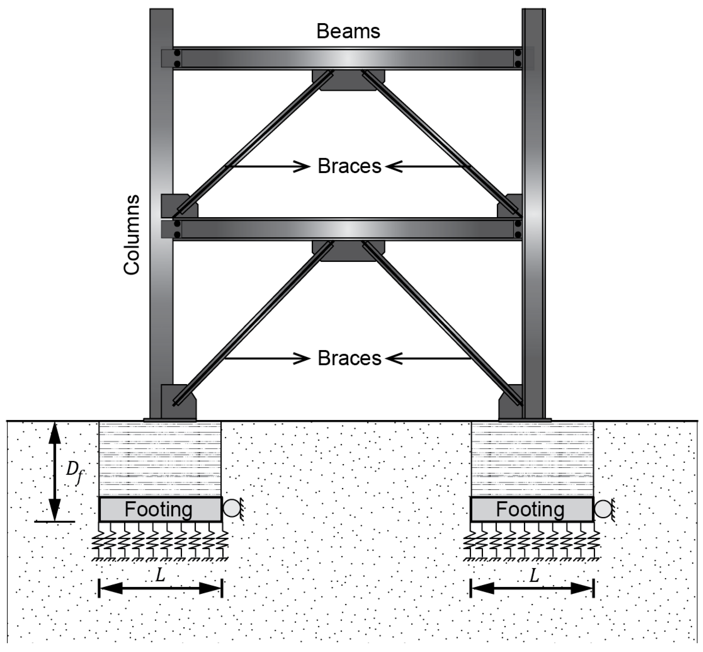
Figure 2.
Proposed backbone curve for modelling the total response of embedded footings for conducting nonlinear analyses.
Figure 2.
Proposed backbone curve for modelling the total response of embedded footings for conducting nonlinear analyses.

Figure 3.
Construction project of an industrial building for the company PAVECA C.A. Valencia, Venezuela. (a) Pit preparation for placing a footing with Df = 2.0 m. (b) Footing placed on site before being covered by the backfill (photographs by Guanchez. E, taken in January 2009). (c) Schematic representation of the construction process according to Kulhawy et al. [28].
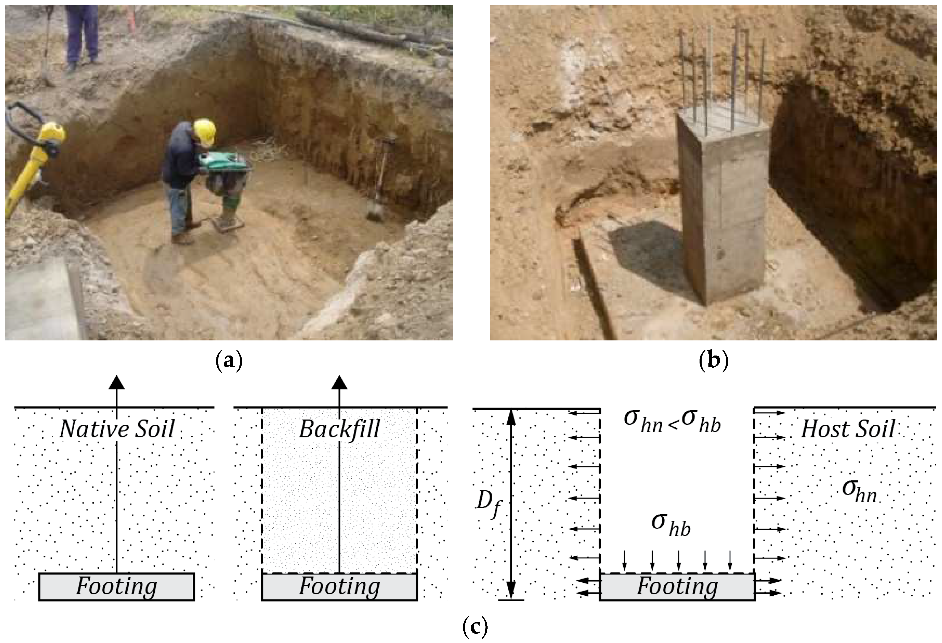
Figure 4.
Distribution of vertical springs below the footing for reproducing the vertical and rotational stiffness simultaneously.
Figure 4.
Distribution of vertical springs below the footing for reproducing the vertical and rotational stiffness simultaneously.

Figure 5.
Representation of variables for estimating δyy_1, δyy_2, δz_1, and δz_2.

Figure 6.
Structural archetype used in this research to perform nonlinear static analyses of fixed and flexible base conditions.
Figure 6.
Structural archetype used in this research to perform nonlinear static analyses of fixed and flexible base conditions.

Figure 7.
(a) Comparison of experimental values reported during the test versus the nonlinear static response curve obtained through FEM analysis. (b) FEM model used for simulations.
Figure 7.
(a) Comparison of experimental values reported during the test versus the nonlinear static response curve obtained through FEM analysis. (b) FEM model used for simulations.
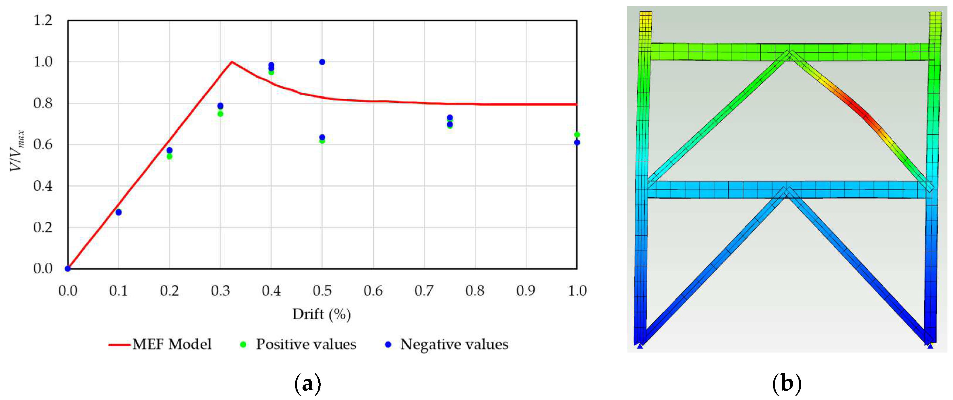
Figure 8.
FEM model used for estimating the nonlinear static response of steel concentrically braced frames supported on a nonlinear flexible base.
Figure 8.
FEM model used for estimating the nonlinear static response of steel concentrically braced frames supported on a nonlinear flexible base.

Figure 9.
Validation of the BNWF model for reproducing the compression responses of footings subjected to large-scale tests [29]. Footing dimensions: (a) 1.0 m × 1.0 m; (b) 1.50 m × 1.50 m; (c) 2.50 m × 2.50 m; (d) 3.0 m × 3.0 m (North); and 3.0 m × 3.0 m (South).
Figure 9.
Validation of the BNWF model for reproducing the compression responses of footings subjected to large-scale tests [29]. Footing dimensions: (a) 1.0 m × 1.0 m; (b) 1.50 m × 1.50 m; (c) 2.50 m × 2.50 m; (d) 3.0 m × 3.0 m (North); and 3.0 m × 3.0 m (South).

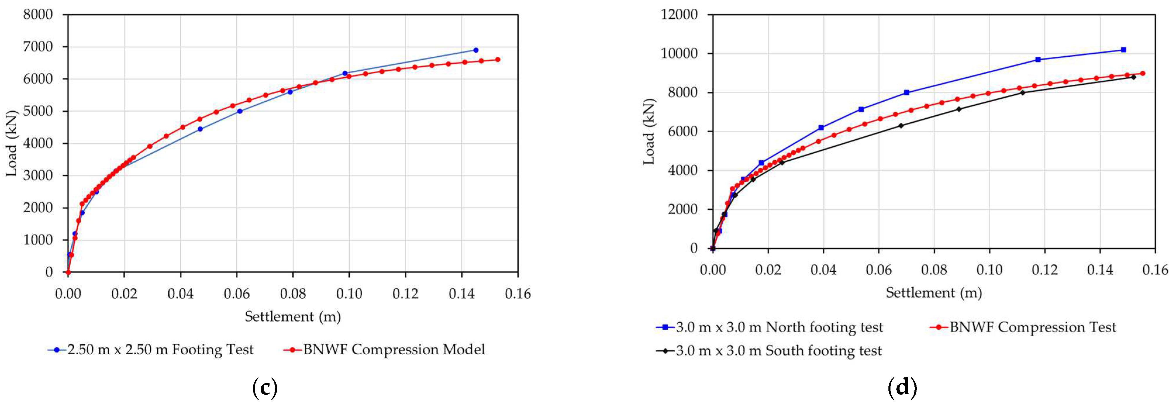
Figure 10.
Distribution of backbone curves along the footing for nonlinear flexible base simulations.
Figure 10.
Distribution of backbone curves along the footing for nonlinear flexible base simulations.
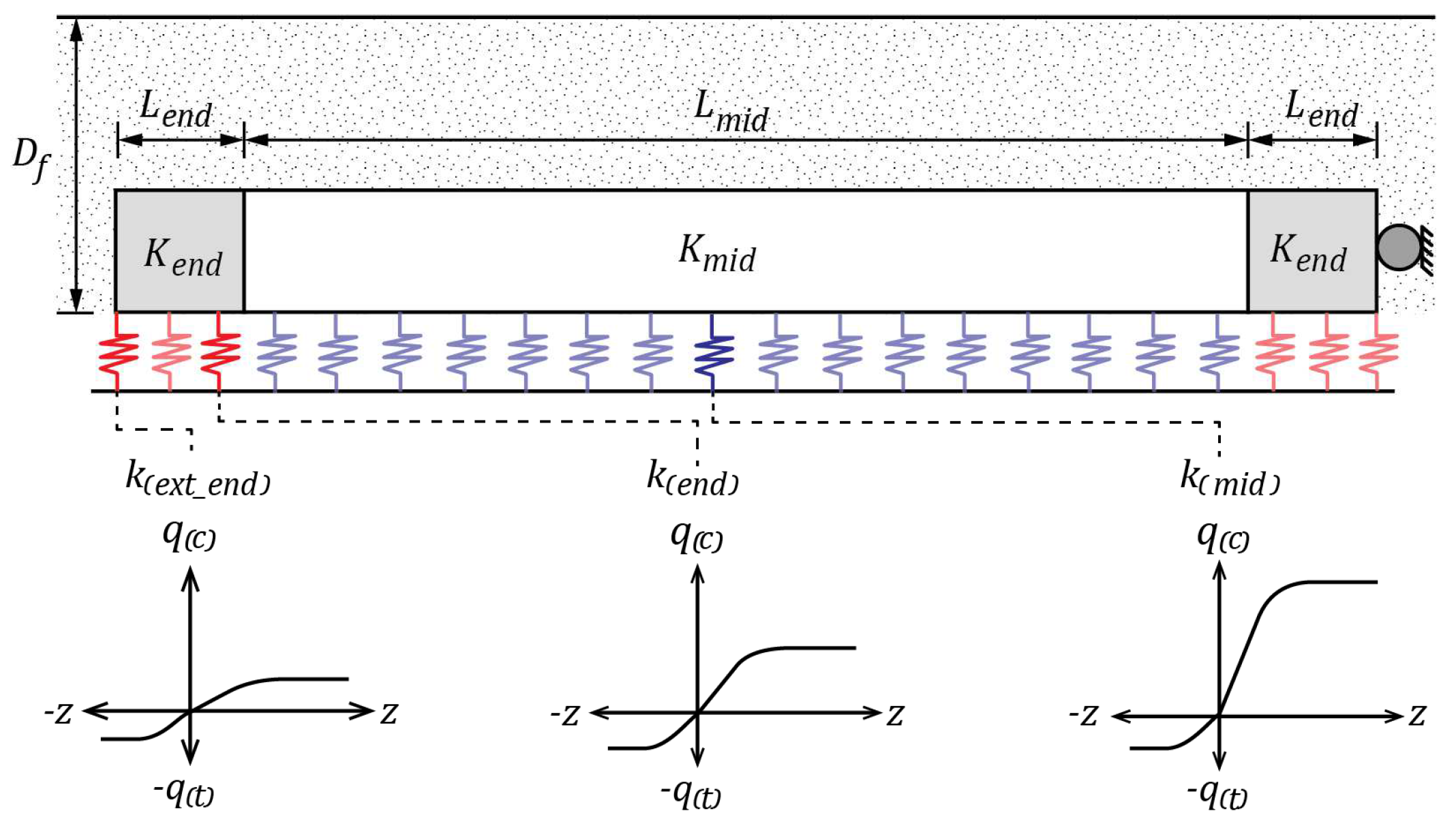
Figure 11.
Backbone curves for Footing 1.0 m × 1.0 m on Soil 3 (K = 2.0): (a) central spring; (b) end spring; and (c) extreme end spring.
Figure 11.
Backbone curves for Footing 1.0 m × 1.0 m on Soil 3 (K = 2.0): (a) central spring; (b) end spring; and (c) extreme end spring.

Figure 12.
Backbone curves for Footing 2.0 m × 2.0 m on Soil 3 (K = 2.0): (a) central spring; (b) end spring; and (c) extreme end spring.
Figure 12.
Backbone curves for Footing 2.0 m × 2.0 m on Soil 3 (K = 2.0): (a) central spring; (b) end spring; and (c) extreme end spring.

Figure 13.
Backbone curves for Footing 3.0 m × 3.0 m on Soil 3 (K = 2.0): (a) central spring; (b) end spring; and (c) extreme end spring.
Figure 13.
Backbone curves for Footing 3.0 m × 3.0 m on Soil 3 (K = 2.0): (a) central spring; (b) end spring; and (c) extreme end spring.
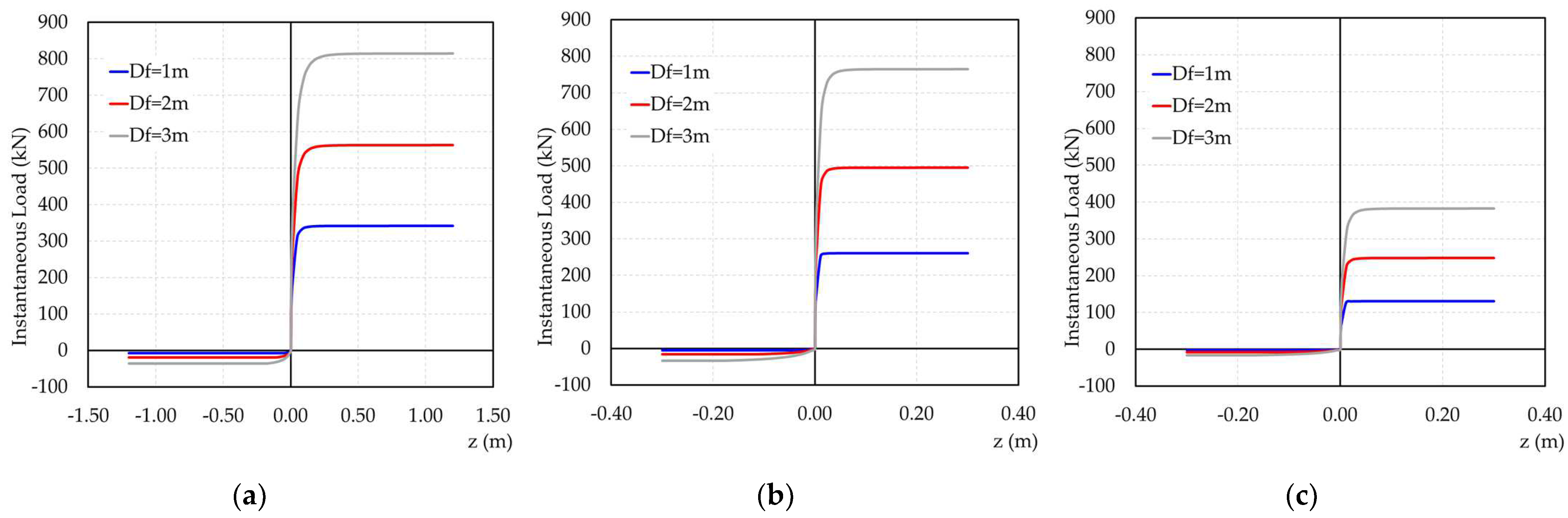
Figure 14.
Variation of quT/qu versus embedment depth Df for each footing dimension and type of soil. Footing dimensions: (a) 1.0 m × 1.0 m; (b) 2.0 m × 2.0 m; (c) 3.0 m × 3.0 m.
Figure 14.
Variation of quT/qu versus embedment depth Df for each footing dimension and type of soil. Footing dimensions: (a) 1.0 m × 1.0 m; (b) 2.0 m × 2.0 m; (c) 3.0 m × 3.0 m.

Figure 15.
Nonlinear static curves of the archetype supported by 2.0 m × 2.0 m footings on (a) Soil Type 1; (b) Soil Type 2; (c) Soil Type 3; (d) Soil Type 4; and (e) Soil Type 5. The values in the text box show the point for 0.8 quT on flexible base conditions compared to the point of failure for the fixed base condition (0.32%).
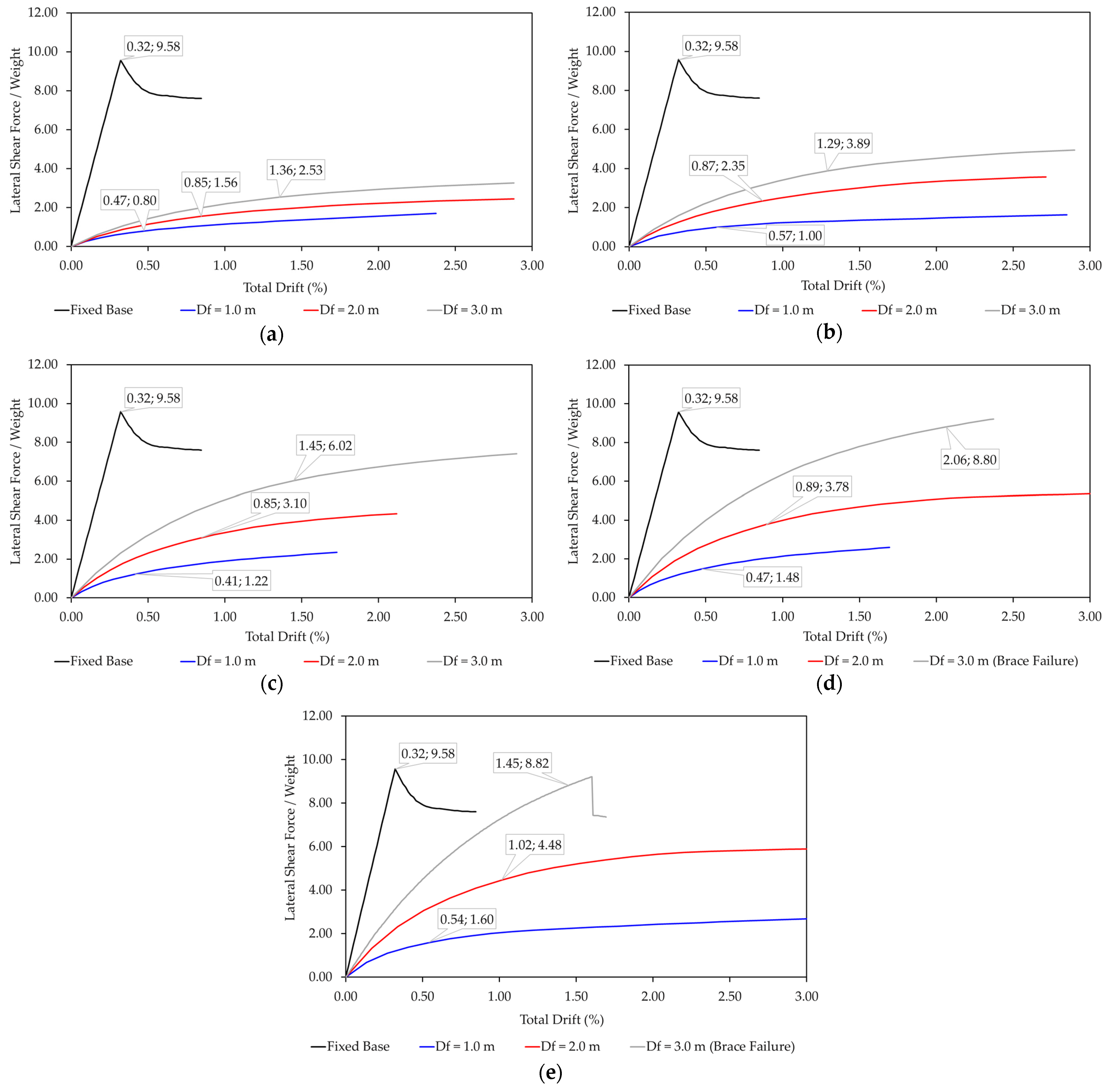
Figure 16.
Plot of the Ki_Flexible Base/Ki_Fixed Base ratio versus the P/Pcr ratio for all cases considered in the simulations. The value Ki_Flexible Base/Ki_Fixed Base = 0.3 represents a threshold between those cases where the uplift of the footing governs (<0.3) or the brace buckles first (>0.3).
Figure 16.
Plot of the Ki_Flexible Base/Ki_Fixed Base ratio versus the P/Pcr ratio for all cases considered in the simulations. The value Ki_Flexible Base/Ki_Fixed Base = 0.3 represents a threshold between those cases where the uplift of the footing governs (<0.3) or the brace buckles first (>0.3).
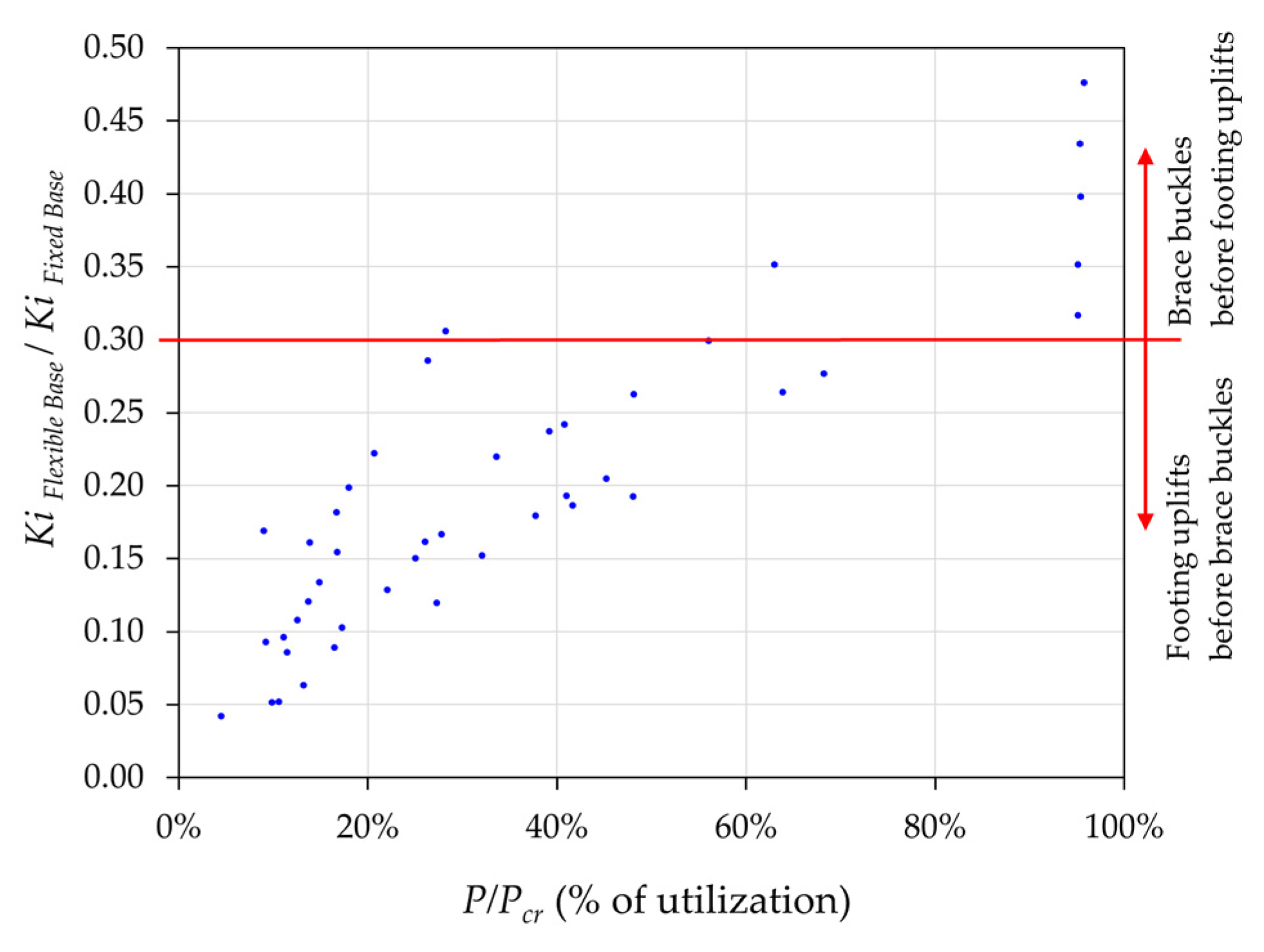
Figure 17.
(a) Capacity curves and (b) P/Pcr ratio versus drift (%) curves for cases where buckling of the brace occurs before the footing uplift mechanism is developed. The values in the text box show the point of imminent failure of the brace (0.95 Pcr) for flexible base conditions compared to the point of failure for the fixed base condition (0.32%).

Figure 18.
Tension curves considered for central springs according to [15] versus the proposed model for a 2.0 m × 2.0 m footing with Df = 2.0 m.
Figure 18.
Tension curves considered for central springs according to [15] versus the proposed model for a 2.0 m × 2.0 m footing with Df = 2.0 m.

Figure 19.
Comparison of nonlinear static curves obtained considering the model according to [15] versus the proposed model. The values in the text box show the point for 0.8 quT on flexible base conditions compared to the point of failure for the fixed base condition (0.32%).
Figure 19.
Comparison of nonlinear static curves obtained considering the model according to [15] versus the proposed model. The values in the text box show the point for 0.8 quT on flexible base conditions compared to the point of failure for the fixed base condition (0.32%).
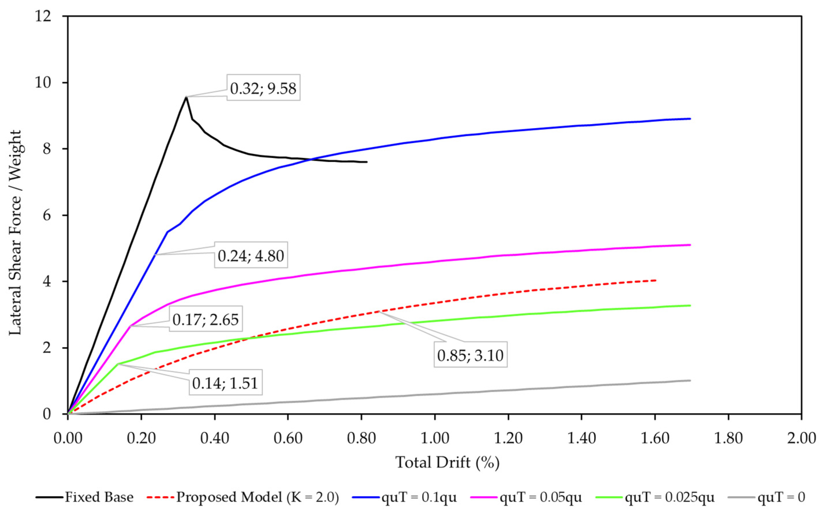
Figure 20.
Comparison of the P/Pcr ratio versus drift ratio curves obtained according to [15] versus the proposed model. The values in the text box show the point for 0.8 quT on flexible base conditions compared to the point of failure for the fixed base condition (0.32%).
Figure 20.
Comparison of the P/Pcr ratio versus drift ratio curves obtained according to [15] versus the proposed model. The values in the text box show the point for 0.8 quT on flexible base conditions compared to the point of failure for the fixed base condition (0.32%).


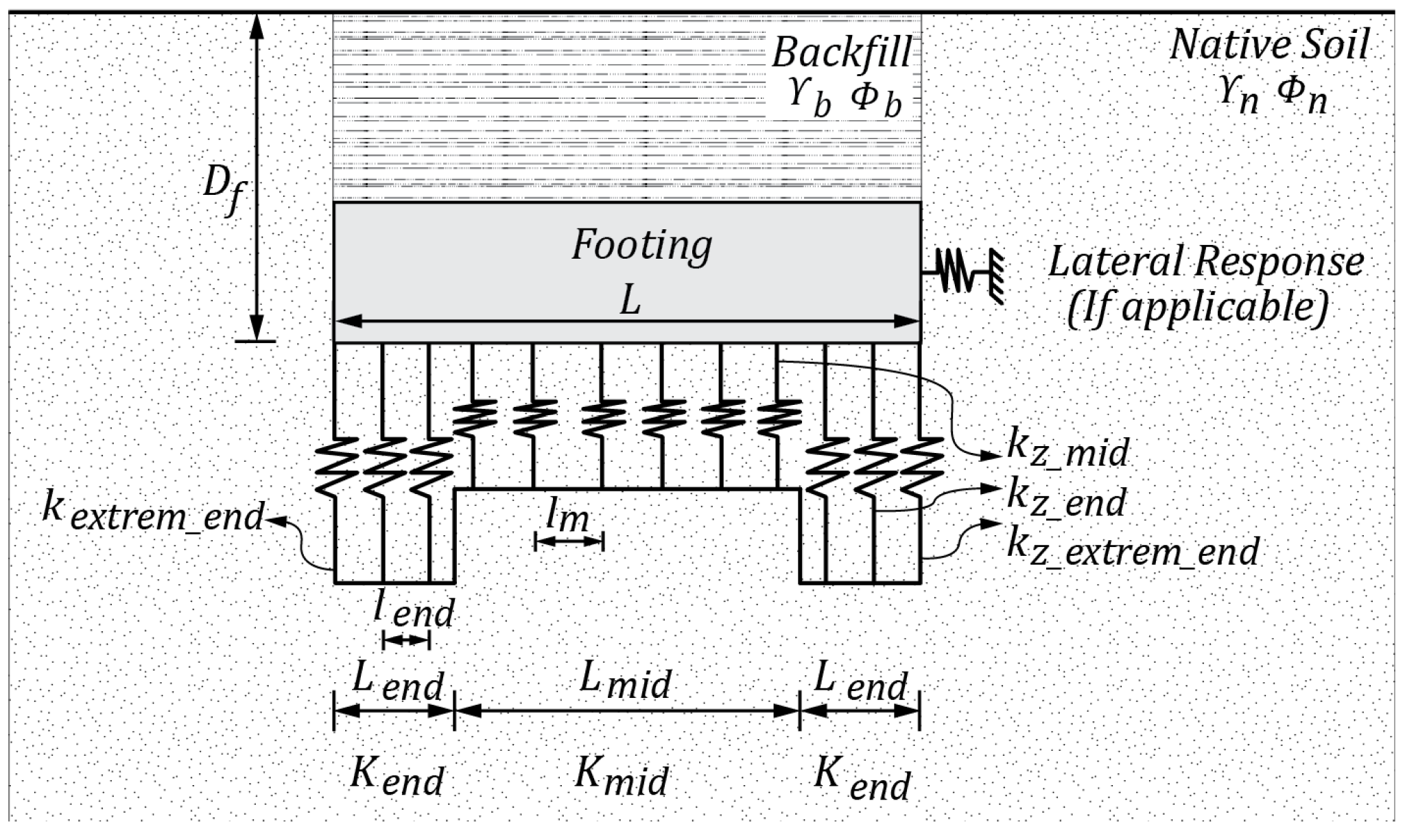
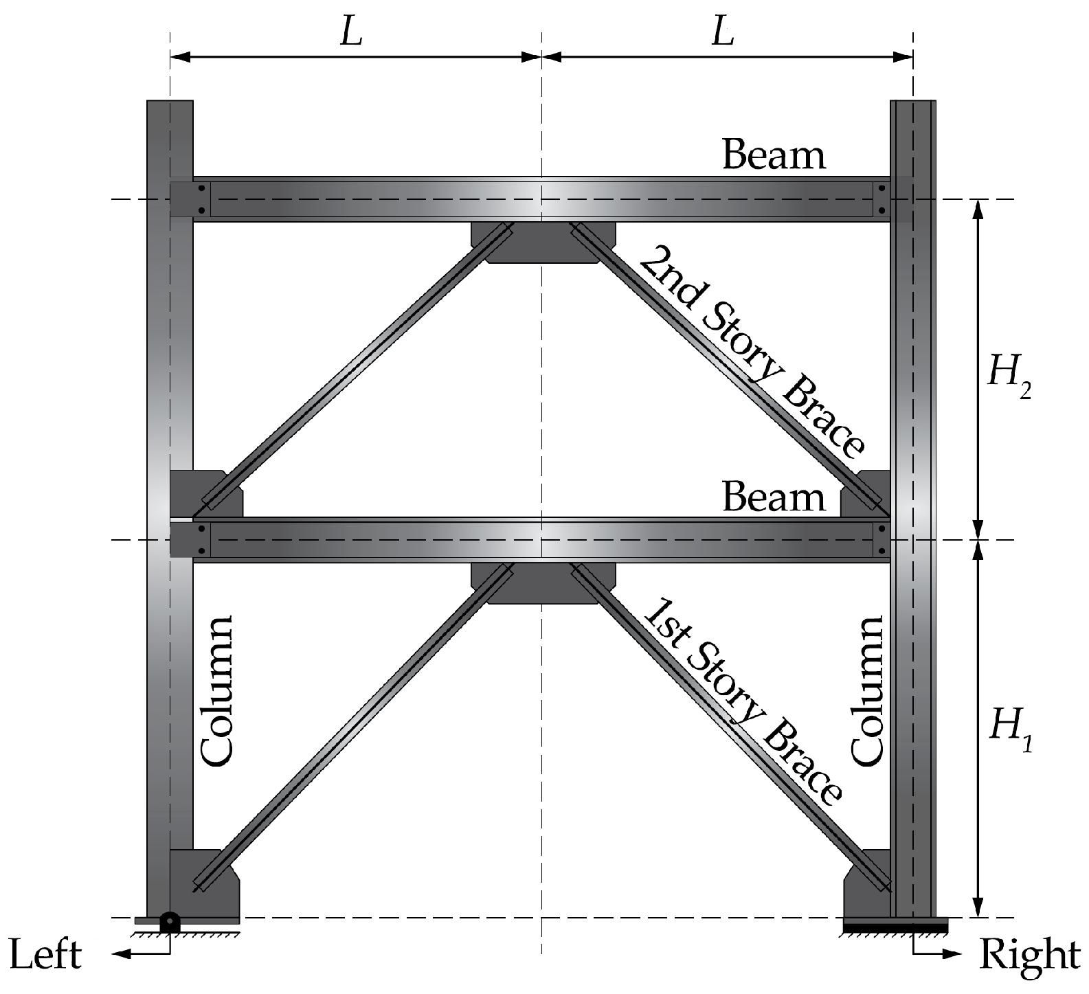
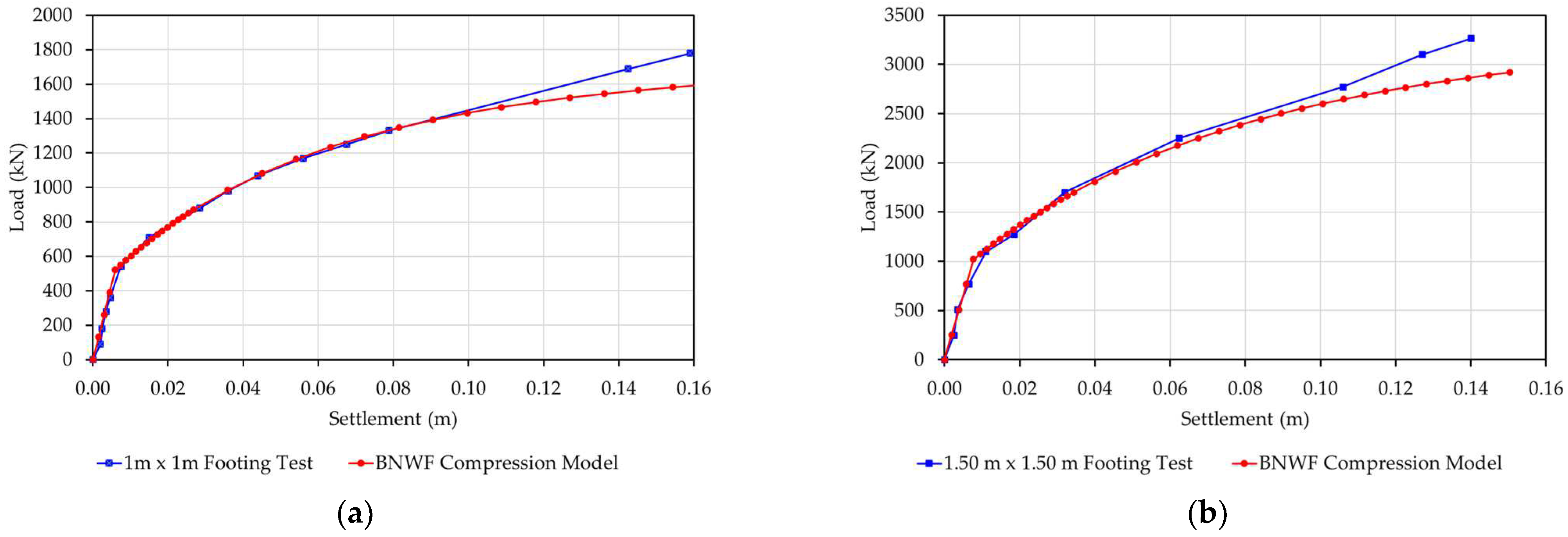
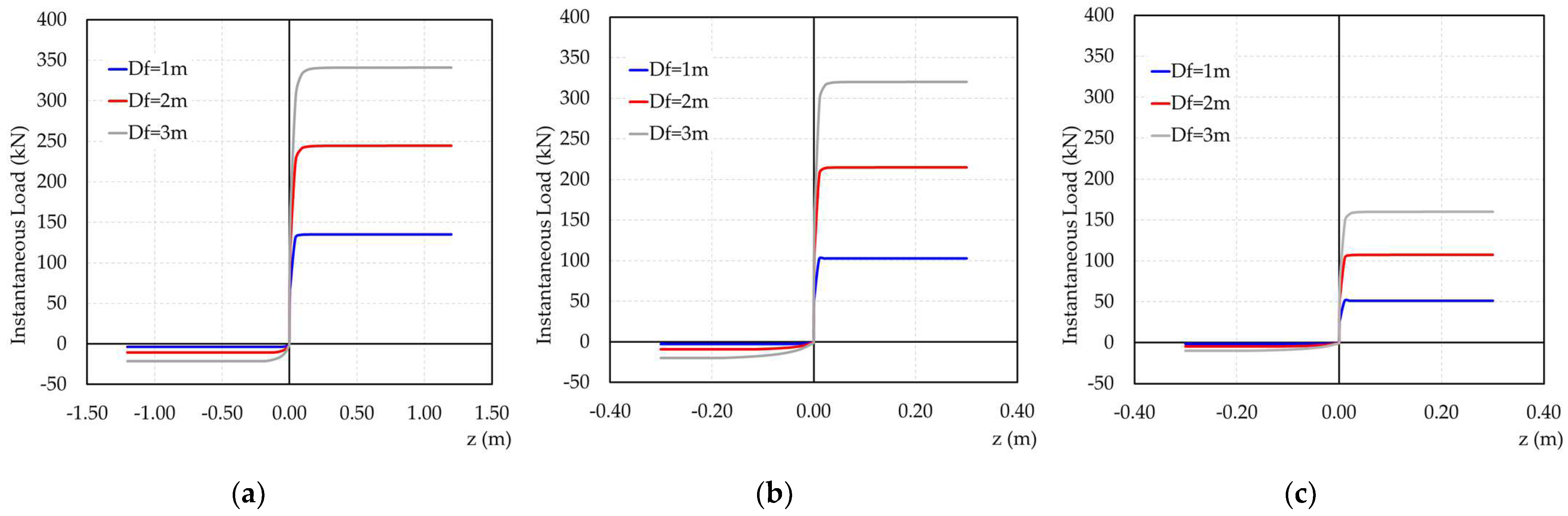
Table 1.
Characteristics of the footings tested by Briaud and Gibbens [29] that were used in the calibration process.
Table 1.
Characteristics of the footings tested by Briaud and Gibbens [29] that were used in the calibration process.
| Footing No. | Embedment Depth (m) | Thickness (m) | Length (m) by Width (m) | Nomenclature Used in This Research |
|---|---|---|---|---|
| 1 | 0.762 | 1.219 | 1.0 × 1.0 | 1.0 m × 1.0 m footing |
| 2 | 0.762 | 1.219 | 1.5 × 1.5 | 1.5 m × 1.5 m footing |
| 3 | 0.889 | 1.346 | 2.5 × 2.5 | 2.5 m × 2.5 m footing |
| 4 | 0.762 | 1.219 | 3.0 × 3.0 | 3.0 m × 3.0 m North footing |
| 5 | 0.711 | 1.168 | 3.0 × 3.0 | 3.0 m × 3.0 m South footing |
Table 2.
Calibration of the elastic portion of the compression curve for tested footings.
| Footing Dimensions (m) | Bearing Capacity Measured qu (kN/m2) | Cr.qu (kN/m2) | Settlement for Cr.qu (m) | Elastic Vertical Stiffness Cr.qu/s (kN/m) | Coefficient G/Gmax | Elastic Vertical Stiffness According to [30] Kz (kN/m) | Elastic Vertical Stiffness According to [31] Kz (kN/m) |
|---|---|---|---|---|---|---|---|
| 1.0 × 1.0 | 1740.0 | 522.0 | 0.006 | 87,000.0 | 0.250 | 86,960.28 | 90,024.96 |
| 1.5 × 1.5 | 1511.0 | 453.3 | 0.008 | 127,490.6 | 0.245 | 127,831.61 | 132,336.69 |
| 2.5 × 2.5 | 1136.0 | 340.8 | 0.005 | 426,000.0 | 0.490 | 426,105.38 | 441,122.31 |
| 3.0 × 3.0 | 1139.0 | 341.7 | 0.007 | 439,328.5 | 0.420 | 438,279.82 | 453,725.81 |
Table 3.
Calibrated constitutive parameters to define the shape of the compression curve for footings.
Table 3.
Calibrated constitutive parameters to define the shape of the compression curve for footings.
| Response Mechanism | Constitutive Parameters | ||
|---|---|---|---|
| Vertical (Compression) | 0.30 | 12.30 | 5.5 |
Table 4.
Material properties of the structural archetype.
| Member | Section | Yield Stress, (MPa) | Ultimate Stress, (MPa) |
|---|---|---|---|
| Column | W10 × 54 | 344.73 | 448.16 |
| Beams | W14 × 53 | 344.73 | 448.16 |
| First story brace | HSS7 × 7 × 1/4 | 356.46 | 466.78 |
| Second story brace | HSS6 × 6 × 3/16 | 337.84 | 450.92 |
Table 5.
Footing dimensions considered for the nonlinear flexible base analysis.
| Plan Dimensions of Footings (m) | Embedment Depth, (m) |
|---|---|
| 1.0 × 1.0 | 1.0 |
| 2.0 | |
| 3.0 | |
| 2.0 × 2.0 | 1.0 |
| 2.0 | |
| 3.0 | |
| 3.0 × 3.0 | 1.0 |
| 2.0 | |
| 3.0 |
Table 6.
Geotechnical parameters considered in the simulations.
| Soil Type | Vs (m/s) | ϕ | γ (kN/m3) | Gmax (Mpa) | G (Mpa) | Density of the Backfill and the Native Soil | ||
|---|---|---|---|---|---|---|---|---|
| 1 | 180 | 30.0 | 18.0 | 59.47 | 14.87 | 0.336 | 0.50 | Loose |
| 2 | 360 | 32.0 | 19.0 | 251.09 | 125.55 | 0.325 | 1.00 | Medium |
| 3 | 540 | 34.0 | 20.0 | 594.70 | 446.02 | 0.315 | 2.00 | Dense |
| 4 | 540 | 36.0 | 21.0 | 594.70 | 446.02 | 0.304 | 3.00 | Very dense |
| 5 | 600 | 38.0 | 22.0 | 807.62 | 726.85 | 0.294 | 3.50 | Very dense |
Table 7.
Matching between vertical and rotational stiffness.
| Plan Dimensions of Footings (m) | Df (m) | Number of Springs | Re (%) | Rk | le/Lf (%) | Var. δyy (%) | Var. δz (%) |
|---|---|---|---|---|---|---|---|
| 1.0 × 1.0 | 1.0 | 51 | 16 | 8.02 | 2 | 2.15 | 4.8 |
| 2.0 | 51 | 18 | 5.74 | 2 | 0.94 | 4.3 | |
| 3.0 | 51 | 19 | 4.60 | 2 | 1.61 | 3.8 | |
| 2.0 × 2.0 | 1.0 | 51 | 16 | 7.62 | 2 | 0.12 | 4.7 |
| 2.0 | 51 | 18 | 6.00 | 2 | 2.69 | 4.4 | |
| 3.0 | 51 | 19 | 5.17 | 2 | 2.39 | 4.2 | |
| 3.0 × 3.0 | 1.0 | 51 | 16 | 7.24 | 2 | 2.25 | 4.5 |
| 2.0 | 51 | 18 | 5.93 | 2 | 2.21 | 4.4 | |
| 3.0 | 51 | 19 | 5.27 | 2 | 3.12 | 4.2 |
Table 8.
Footing backbone curves considered in the simulations for Soil 3 (K = 2.0).
| Footing Dimensions (m) | Df (m) | qu (kN/m2) | Kz_emb (kN/m) | Kyy_emb (kN-m/rad) | quT (kN/m2) | quT/qu (%) |
|---|---|---|---|---|---|---|
| 1.0 × 1.0 | 1.0 | 1490.77 | 2,324,513.35 | 747,722.49 | 65.85 | 4.42 |
| 2.0 | 2790.54 | 2,742,199.34 | 714,829.05 | 219.81 | 7.88 | |
| 3.0 | 4172.64 | 3,159,885.33 | 708,361.87 | 463.08 | 11.10 | |
| 2.0 × 2.0 | 1.0 | 1607.93 | 3,893,682.37 | 4,805,919.55 | 43.52 | 2.71 |
| 2.0 | 2981.54 | 4,278,037.28 | 4,632,571.29 | 130.50 | 4.38 | |
| 3.0 | 4212.59 | 4,662,392.19 | 4,598,489.28 | 262.14 | 6.22 | |
| 3.0 × 3.0 | 1.0 | 1811.24 | 5,448,635.37 | 14,534,333.89 | 36.08 | 1.99 |
| 2.0 | 3055.63 | 5,819,400.50 | 1,407,6780.98 | 100.73 | 3.30 | |
| 3.0 | 4472.31 | 6,190,165.63 | 13,986,821.49 | 195.16 | 4.36 |
Table 9.
Ratio between the drift of the flexible base models at the point of imminent uplift Drift_Flex(0.8quT), and the drift of the fixed base model at the point of brace yielding Drift_Fixed(0.32%), for different soil types, embedment depths Df, and footing dimensions.
Table 9.
Ratio between the drift of the flexible base models at the point of imminent uplift Drift_Flex(0.8quT), and the drift of the fixed base model at the point of brace yielding Drift_Fixed(0.32%), for different soil types, embedment depths Df, and footing dimensions.
| Soil Type | Vs (m/s) | K | Plan Dimensions (m) | Df (m) | Roof Displacement for 0.8 quT (mm) | Drift_Flex for 0.8 quT (%) | Ratio Drift_Flex(0.8quT)/ Drift_Fixed(0.32%) |
|---|---|---|---|---|---|---|---|
| Soil 1 | 180 | 0.5 | 1.0 × 1.0 | 1.0 | 27.0 | 0.457 | 1.42 |
| 2.0 | 52.0 | 0.881 | 2.74 | ||||
| 3.0 | 78.0 | 1.322 | 4.11 | ||||
| 2.0 × 2.0 | 1.0 | 28.0 | 0.474 | 1.47 | |||
| 2.0 | 50.0 | 0.847 | 2.63 | ||||
| 3.0 | 80.0 | 1.355 | 4.21 | ||||
| 3.0 × 3.0 | 1.0 | 32.0 | 0.542 | 1.68 | |||
| 2.0 | 54.0 | 0.915 | 2.84 | ||||
| 3.0 | 75.0 | 1.271 | 3.95 | ||||
| Soil 2 | 360 | 1.0 | 1.0 × 1.0 | 1.0 | 27.0 | 0.457 | 1.42 |
| 2.0 | 50.4 | 0.854 | 2.65 | ||||
| 3.0 | 72.5 | 1.228 | 3.82 | ||||
| 2.0 × 2.0 | 1.0 | 33.6 | 0.569 | 1.77 | |||
| 2.0 | 51.2 | 0.867 | 2.69 | ||||
| 3.0 | 76.0 | 1.288 | 4.00 | ||||
| 3.0 × 3.0 | 1.0 | 2.56 | 0.043 | 0.13 | |||
| 2.0 | 4.95 | 0.083 | 0.26 | ||||
| 3.0 | 7.92 | 0.134 | 0.42 | ||||
| Soil 3 | 540 | 2.0 | 1.0 × 1.0 | 1.0 | 25.8 | 0.437 | 1.36 |
| 2.0 | 51.6 | 0.874 | 2.72 | ||||
| 3.0 | 76.0 | 1.288 | 4.00 | ||||
| 2.0 × 2.0 | 1.0 | 24.4 | 0.414 | 1.29 | |||
| 2.0 | 50.0 | 0.847 | 2.63 | ||||
| 3.0 | 85.5 | 1.449 | 4.50 | ||||
| 3.0 × 3.0 | 1.0 | 25.2 | 0.427 | 1.33 | |||
| 2.0 | 58.5 | 0.991 | 3.08 | ||||
| 3.0 | Brace failure occurs first | ||||||
| Soil 4 | 540 | 3.0 | 1.0 × 1.0 | 1.0 | 26.4 | 0.447 | 1.39 |
| 2.0 | 52.0 | 0.881 | 2.74 | ||||
| 3.0 | 80.0 | 1.355 | 4.21 | ||||
| 2.0 × 2.0 | 1.0 | 28.0 | 0.474 | 1.47 | |||
| 2.0 | 52.8 | 0.894 | 2.78 | ||||
| 3.0 | Brace failure occurs first | ||||||
| 3.0 × 3.0 | 1.0 | 28.0 | 0.474 | 1.47 | |||
| 2.0 | 54.0 | 0.915 | 2.84 | ||||
| 3.0 | Brace failure occurs first | ||||||
| Soil 5 | 600 | 3.5 | 1.0 × 1.0 | 1.0 | 25.6 | 0.436 | 1.36 |
| 2.0 | 53.9 | 0.914 | 2.84 | ||||
| 3.0 | 82.0 | 1.389 | 4.32 | ||||
| 2.0 × 2.0 | 1.0 | 32.0 | 0.542 | 1.68 | |||
| 2.0 | 60.0 | 1.016 | 3.16 | ||||
| 3.0 | Brace failure occurs first | ||||||
| 3.0 × 3.0 | 1.0 | 28.0 | 0.474 | 1.47 | |||
| 2.0 | 92.4 | 1.566 | 4.86 | ||||
| 3.0 | Brace failure occurs first | ||||||
Table 10.
Ratio of the initial stiffness of the flexible base model Ki_Flexible Base with respect to the initial stiffness of the fixed base model Ki_Fixed Base for cases where the brace buckling mechanism governs.
Table 10.
Ratio of the initial stiffness of the flexible base model Ki_Flexible Base with respect to the initial stiffness of the fixed base model Ki_Fixed Base for cases where the brace buckling mechanism governs.
| Soil Type | Footing Dimensions (m) | Df (m) | Drift for 0.95Pcr (%) | Ki_Flexible Base (kN/m) | Ki_Flexible Base/ Ki_Fixed Base |
|---|---|---|---|---|---|
| Soil 5 | 3.0 × 3.0 | 3.0 | 0.74 | 35,346.30 | 0.476 |
| Soil 4 | 3.0 | 0.88 | 32,246.67 | 0.434 | |
| Soil 3 | 3.0 | 1.10 | 28,998.75 | 0.390 | |
| Soil 5 | 2.0 × 2.0 | 3.0 | 1.45 | 26,094.00 | 0.351 |
| Soil 4 | 3.0 | 2.06 | 23,537.38 | 0.317 |
Table 11.
Ultimate tension capacity quT estimated as a percentage of bearing capacity qu versus the ultimate tension capacity estimated using the model proposed in this research.
Table 11.
Ultimate tension capacity quT estimated as a percentage of bearing capacity qu versus the ultimate tension capacity estimated using the model proposed in this research.
| Soil Type | Footing Dimensions (m) | Df (m) | %qu | quT as %qu (kN) | quT According to Equation (5) (kN) |
|---|---|---|---|---|---|
| Soil 3 | 2.0 × 2.0 | 1.0 | 0 | 0 | 174.10 |
| 2.5 | 160.79 | ||||
| 5.0 | 321.59 | ||||
| 10.0 | 643.17 | ||||
| 2.0 | 0 | 0 | 522.02 | ||
| 2.5 | 298.15 | ||||
| 5.0 | 596.31 | ||||
| 10.0 | 1192.62 | ||||
| 3.0 | 0 | 0 | 1048.56 | ||
| 2.5 | 421.25 | ||||
| 5.0 | 842.52 | ||||
| 10.0 | 1685.04 |
Table 12.
Lateral stiffness variation of the structure considering the model according to [15].
Table 12.
Lateral stiffness variation of the structure considering the model according to [15].
| Soil Type | Footing Dimensions (m) | Df (m) | %qu | K0.8quT (kN/m) | Ki (kN/m) | K0.8quT/Ki |
|---|---|---|---|---|---|---|
| Soil 3 | 2.0 × 2.0 | 1.0 | 2.5 | 28,464.44 | 28,467.50 | 1.000 |
| 5.0 | 47,999.48 | 48,007.81 | 1.000 | |||
| 10.0 | 50,255.73 | 50,266.67 | 1.000 | |||
| 2.0 | 2.5 | 27,769.88 | 27,790.50 | 0.999 | ||
| 5.0 | 38,891.50 | 38,905.00 | 1.000 | |||
| 10.0 | 50,342.86 | 50,305.00 | 1.000 | |||
| 3.0 | 2.5 | 26,561.60 | 26,585.50 | 0.999 | ||
| 5.0 | 38,233.21 | 38,255.50 | 0.999 | |||
| 10.0 | 43,374.39 | 49,581.00 | 0.875 |
Table 13.
Lateral stiffness variation of the structure considering the proposed model.
| Soil Type | Footing Dimensions (m) | Df (m) | %qu | K0.8quT (kN/m) | Ki (kN/m) | K0.8quT/Ki |
|---|---|---|---|---|---|---|
| Soil 3 | 2.0 × 2.0 | 1.0 | N/A | 7330.19 | 11,973.53 | 0.61 |
| 2.0 | N/A | 9101.90 | 16,320.60 | 0.56 | ||
| 3.0 | N/A | 10,337.46 | 19,611.26 | 0.53 |
Table 14.
Ductility variation of nonlinear flexible base models.
| Soil Type | Footing Dimensions (m) | Df (m) | δu (%) | δy_eff (%) | μT | Var. (%) |
|---|---|---|---|---|---|---|
| Soil 1 | 1.0 × 1.0 | 1.0 | 0.457 | 0.274 | 1.67 | 28.45 |
| 2.0 | 0.881 | 0.508 | 1.73 | 33.34 | ||
| 3.0 | 1.322 | 0.620 | 2.13 | 63.91 | ||
| 2.0 × 2.0 | 1.0 | 0.474 | 0.289 | 1.64 | 26.39 | |
| 2.0 | 0.847 | 0.506 | 1.67 | 28.80 | ||
| 3.0 | 1.355 | 0.708 | 1.92 | 47.42 | ||
| 3.0 × 3.0 | 1.0 | 0.542 | 0.330 | 1.65 | 26.60 | |
| 2.0 | 0.915 | 0.521 | 1.76 | 35.12 | ||
| 3.0 | 1.271 | 0.780 | 1.63 | 25.40 | ||
| Soil 2 | 1.0 × 1.0 | 1.0 | 0.457 | 0.322 | 1.42 | 9.26 |
| 2.0 | 0.854 | 0.493 | 1.73 | 33.23 | ||
| 3.0 | 1.228 | 0.613 | 2.00 | 54.20 | ||
| 2.0 × 2.0 | 1.0 | 0.569 | 0.346 | 1.65 | 26.57 | |
| 2.0 | 0.867 | 0.486 | 1.78 | 37.26 | ||
| 3.0 | 1.288 | 0.697 | 1.85 | 42.10 | ||
| 3.0 × 3.0 | 1.0 | 0.433 | 0.277 | 1.57 | 20.43 | |
| 2.0 | 0.839 | 0.516 | 1.63 | 25.03 | ||
| 3.0 | 1.342 | 0.790 | 1.70 | 30.66 | ||
| Soil 3 | 1.0 × 1.0 | 1.0 | 0.437 | 0.290 | 1.51 | 15.89 |
| 2.0 | 0.874 | 0.479 | 1.83 | 40.48 | ||
| 3.0 | 1.288 | 0.646 | 2.00 | 53.48 | ||
| 2.0 × 2.0 | 1.0 | 0.414 | 0.254 | 1.63 | 25.65 | |
| 2.0 | 0.847 | 0.473 | 1.79 | 37.93 | ||
| 3.0 | 1.449 | 0.764 | 1.90 | 45.93 | ||
| 3.0 × 3.0 | 1.0 | 0.427 | 0.289 | 1.48 | 13.70 | |
| 2.0 | 0.991 | 0.589 | 1.68 | 29.42 | ||
| 3.0 | 1.098 | 0.767 | 1.43 | 10.12 | ||
| Soil 4 | 1.0 × 1.0 | 1.0 | 0.447 | 0.289 | 1.55 | 19.16 |
| 2.0 | 0.881 | 0.476 | 1.85 | 42.48 | ||
| 3.0 | 1.355 | 0.663 | 2.04 | 57.23 | ||
| 2.0 × 2.0 | 1.0 | 0.474 | 0.273 | 1.74 | 33.96 | |
| 2.0 | 0.894 | 0.523 | 1.71 | 31.57 | ||
| 3.0 | 2.064 | 0.930 | 2.22 | 70.76 | ||
| 3.0 × 3.0 | 1.0 | 0.474 | 0.282 | 1.68 | 29.29 | |
| 2.0 | 0.915 | 0.565 | 1.62 | 24.52 | ||
| 3.0 | 0.884 | 0.690 | ≅1.3 | ≅0 | ||
| Soil 5 | 1.0 × 1.0 | 1.0 | 0.436 | 0.284 | 1.54 | 18.17 |
| 2.0 | 0.914 | 0.484 | 1.89 | 45.35 | ||
| 3.0 | 1.389 | 0.692 | 2.01 | 54.42 | ||
| 2.0 × 2.0 | 1.0 | 0.542 | 0.317 | 1.71 | 31.72 | |
| 2.0 | 1.016 | 0.571 | 1.78 | 36.97 | ||
| 3.0 | 1.449 | 0.840 | 1.73 | 32.70 | ||
| 3.0 × 3.0 | 1.0 | 0.474 | 0.284 | 1.67 | 28.49 | |
| 2.0 | 1.566 | 0.743 | 2.11 | 62.22 | ||
| 3.0 | 0.741 | 0.628 | ≅1.3 | ≅0 |
Disclaimer/Publisher’s Note: The statements, opinions and data contained in all publications are solely those of the individual author(s) and contributor(s) and not of MDPI and/or the editor(s). MDPI and/or the editor(s) disclaim responsibility for any injury to people or property resulting from any ideas, methods, instructions or products referred to in the content. |
© 2024 by the authors. Licensee MDPI, Basel, Switzerland. This article is an open access article distributed under the terms and conditions of the Creative Commons Attribution (CC BY) license (https://creativecommons.org/licenses/by/4.0/).
Share and Cite
MDPI and ACS Style
Guanchez, E.; Weyler, R.; Sanchez, M. Influence of the Uplifting Mechanism of Embedded Footings on the Nonlinear Static Response of Steel Concentrically Braced Frames. Buildings 2024, 14, 1145. https://doi.org/10.3390/buildings14041145
AMA Style
Guanchez E, Weyler R, Sanchez M. Influence of the Uplifting Mechanism of Embedded Footings on the Nonlinear Static Response of Steel Concentrically Braced Frames. Buildings. 2024; 14(4):1145. https://doi.org/10.3390/buildings14041145
Chicago/Turabian StyleGuanchez, Edinson, Rafael Weyler, and Montserrat Sanchez. 2024. "Influence of the Uplifting Mechanism of Embedded Footings on the Nonlinear Static Response of Steel Concentrically Braced Frames" Buildings 14, no. 4: 1145. https://doi.org/10.3390/buildings14041145
Note that from the first issue of 2016, this journal uses article numbers instead of page numbers. See further details here.