
Resilience-Oriented Planning of Urban Distribution System Source–Network–Load–Storage in the Context of High-Penetrated Building-Integrated Resources
Abstract
:1. Introduction
1.1. Background and Motivation
1.2. Literature Review
1.3. Contribution and Paper Organization
2. Problem Formulation
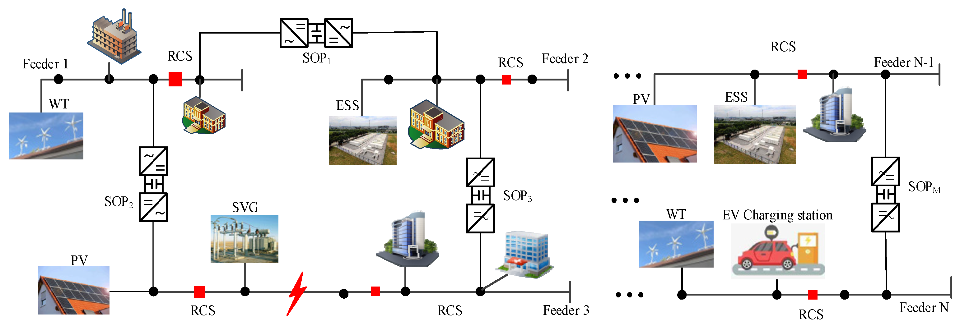
2.1. Source–Network–Load–Storage Coordination in the Context of High-Penetrated Building-Integrated Resources
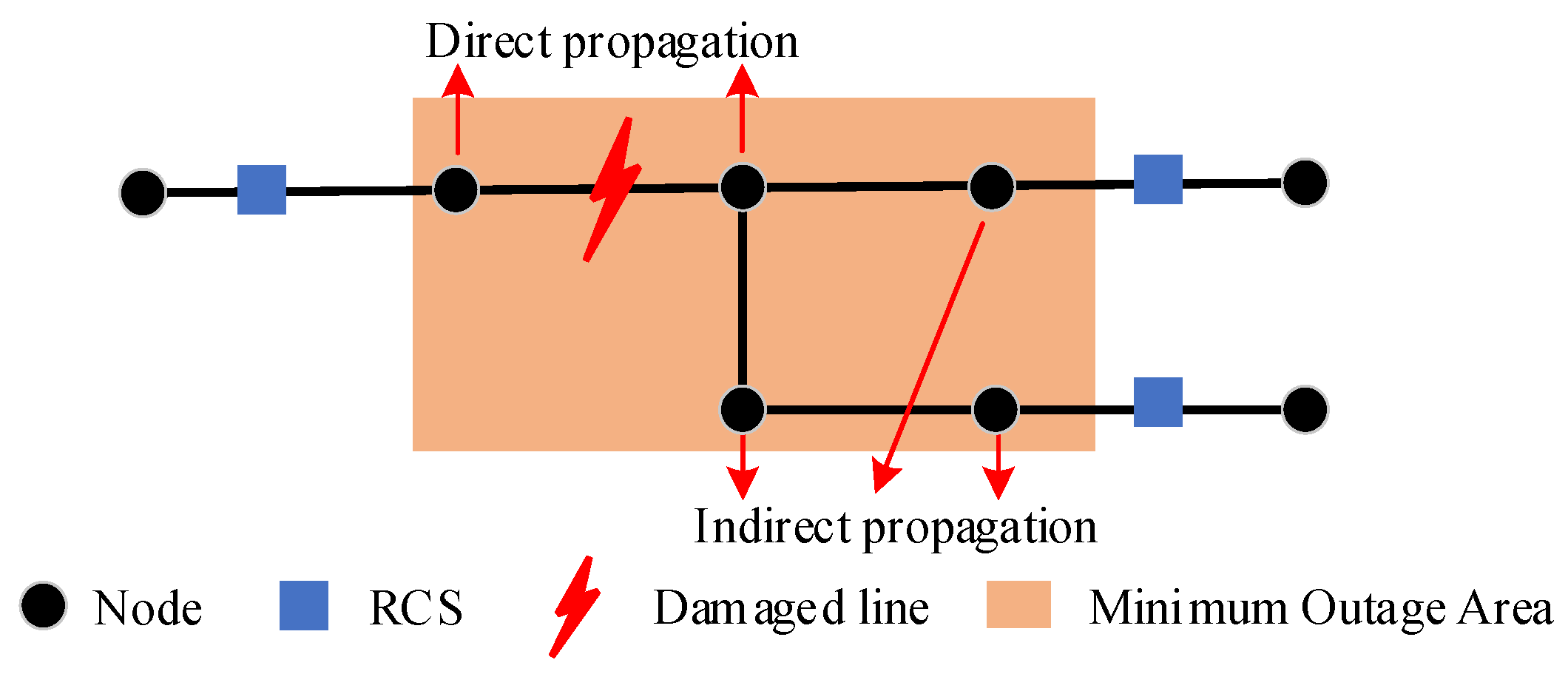
2.2. Fault Isolation and Recovery
3. Resilience-Oriented Planning of Source–Network–Load–Storage
3.1. Resilience-Oriented Planning Objective Function
3.2. Constraints of Source–Network–Load–Storage
3.3. Multi-Dimensional Evaluation
3.4. MILP Reformulation
3.5. Two-Stage Planning–Operation Method
4. Case Study
4.1. Base Data
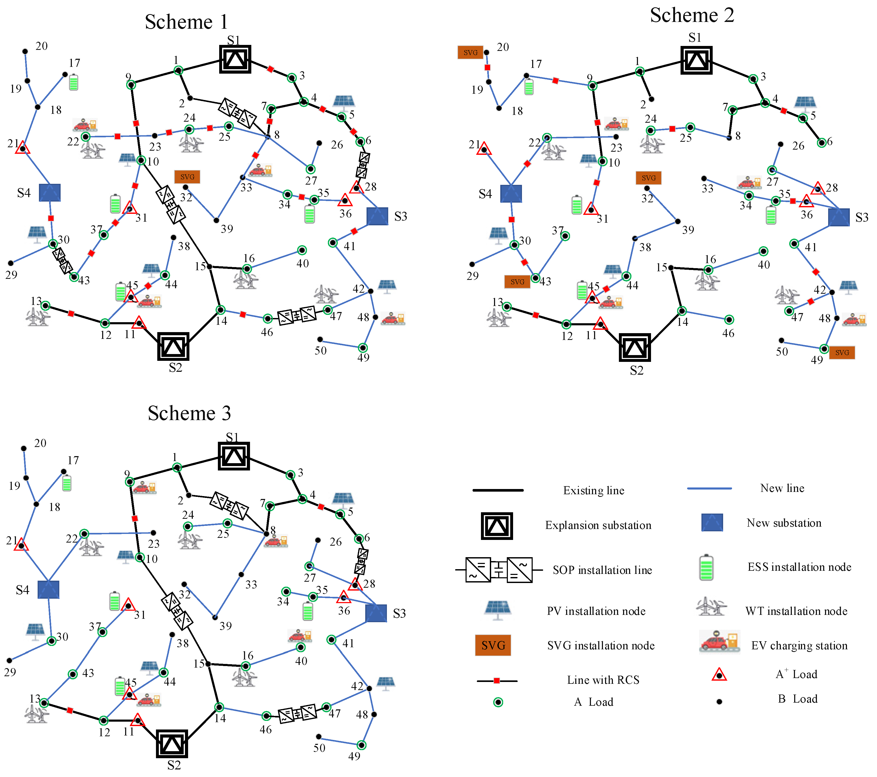
4.2. Analysis of Planning Results
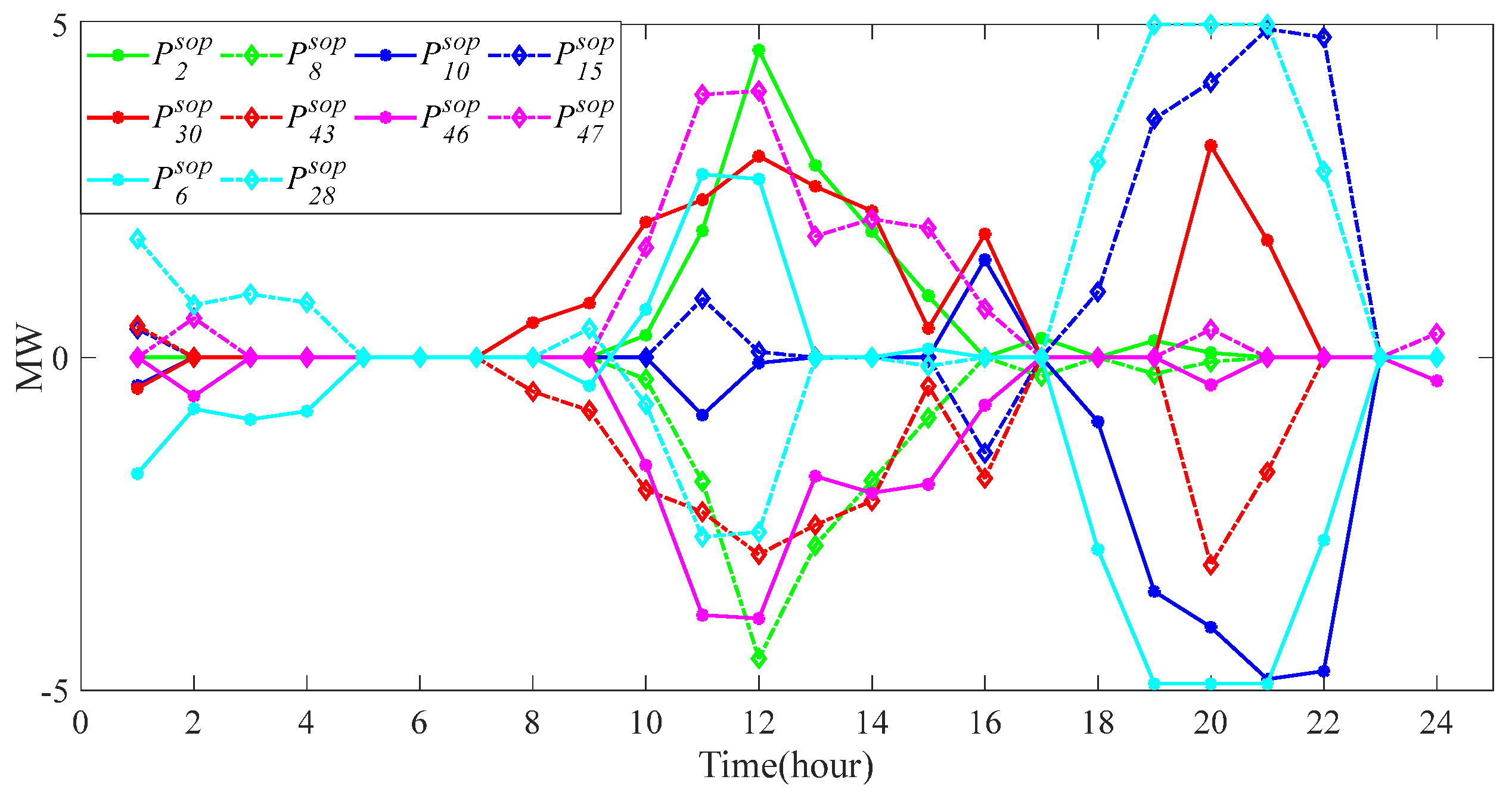
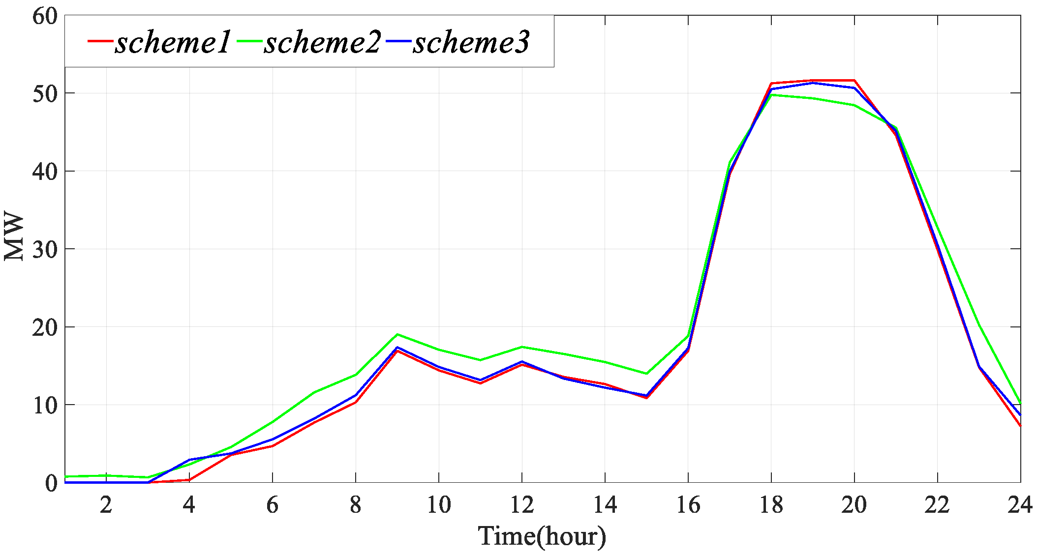
4.3. Analysis of Operational Results
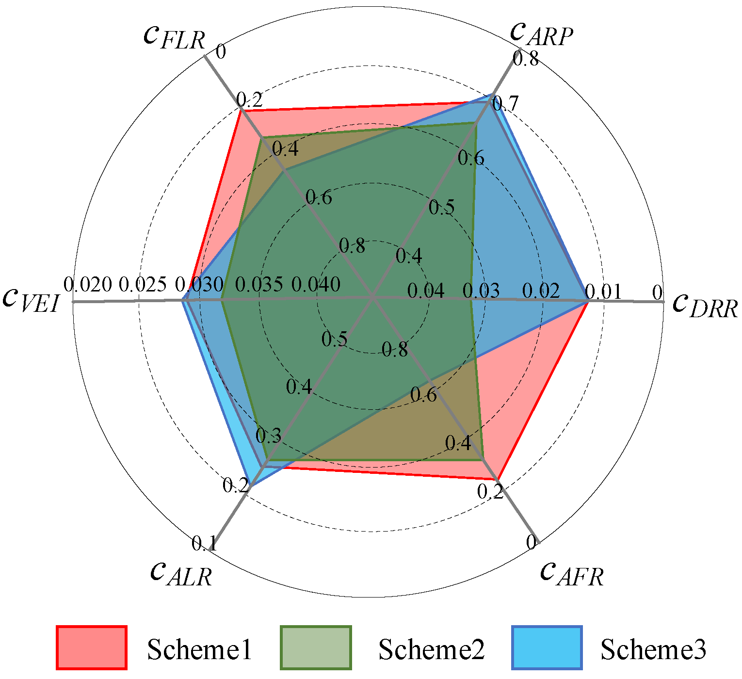
4.4. Multi-Dimensional Comparisons
5. Conclusions and Discussion
- The contribution of SOP integration to system flexibility and thus to the system dependency on ESSs and SVGs results in a decrease in installed capacity. By exploiting the optimal synergies among different components, the coordination of source–network–load–storage can enhance the system dispatchability in spatial (RES accommodation) and temporal (energy storage) scales, thereby giving rise to at most 6.7% cost reduction.
- SOPs have the capability to provide reactive voltage support and power flow transfer to the terminal nodes. By considering various fault scenarios during the planning stages, the node failure rates can be significantly reduced with the strengthened interconnectivity from SOPs, thereby mitigating the load losses incurred.
- The proposed resilience-oriented planning scheme can outperform others on system economy, flexibility, and resilience indices, which exhibits huge development and application potentialities in urban distribution systems.
- Multi-energy source–network–load–storage coordination: Compared with power systems, gas and heating (cold) systems have larger time constants and significant time delays. The multi-energy source–network–load–storage coordination may need to be described by algebraic equations (electricity) and transient differential equations (gas, heat). With large-scale RES integration, multi-energy source–network–load–storage planning problems have evolved into problems involving multiple time scales of years, months/weeks, and short-term operations.
- Disturbances from various natural disasters: Frequent natural disasters pose significant challenges to the urban distribution system, posing a severe threat to urban energy security and societal development. Worst of all is the combined impact of multiple weather- and climate-driven natural disasters, including typhoons, thunderstorms, floods, etc. Such disturbances from various natural disasters would contribute to considerable difficulty in pre-deployment and post-disaster recovery.
Author Contributions
Funding
Data Availability Statement
Conflicts of Interest
Nomenclature
| Abbreviations | ||
| BIPVs | Building-integrated photovoltaics | |
| BIWT | Building-integrated wind turbine | |
| ESS | Energy storage system | |
| EV | Electric vehicle | |
| MILP | Mixed-integer linear programming | |
| PV | Photovoltaic | |
| RESs | Renewable energy sources | |
| RCSs | Remote-controlled switches | |
| SVG | Static var generator | |
| SOP | Soft open point | |
| WT | Wind turbine | |
| Indices and sets | ||
| t, s | Index for time, scenario | |
| i, j | Index for node and branch | |
| Ωs, Ωf | Set of normal and fault scenarios | |
| Ωwt, Ωpv, Ωsvg, Ωes | Set of BIWT, BIPV, SVG, ESS candidate nodes | |
| Ωsub, Ωesub, | Set of constructable and expandable substation nodes | |
| ΩL, Ωn | Set of lines and load candidate nodes | |
| Ωev, Ωev,i | Set of EV charging station nodes and candidate nodes | |
| Parameters | ||
| Loss coefficients of SOP | ||
| BIWT and BIPV outputs | ||
| βmin, βmax | Lower and upper limits of SVG | |
| , | Maximum installed capacities of BIWT, BIPV, SVG, ESS and SOP | |
| λWT, λPV | Maximum allowable BIWT and BIPV curtailments | |
| Ksub | Maximum load ratio of the substation | |
| Constructable, initial, and expandable substation capacities | ||
| n, ns0, N | Total numbers of nodes, existing substations, and added nodes | |
| ξi | Maximum load shedding ratio | |
| , | Active and reactive load | |
| kch, kdis, ηch, ηdis | ESS charging and discharging depths and efficiency | |
| μmin, μmax | Upper and lower bounds of ESS capacity | |
| EV charging station load | ||
| Umin, Umax, V0 | Minimum, maximum, and standard voltage | |
| rij, xij, Sij | Resistance, reactance and capacity of lines ij | |
| fij,s | Fault of the line ij | |
| R, Rrcs | Maximum numbers of restored lines and installed RCSs | |
| Tf, Tre | Time of fault occurrence and recovery | |
| , , , , ,,, , | Unit investment costs of BIWT, BIPVs, ESS, SOP, SVG, RCS, line constructed substation, and expanded substation | |
| fwt, fpv | Penalties for BIWT and BIPV curtailment | |
| Battery degradation cost | ||
| , | Annual maintenance costs of BIWT, BIPVs, SOP, SVG and line | |
| , | Load shedding penalties in normal and fault scenarios | |
| ρs, ρsf | Probabilities in normal and fault scenarios | |
| pt | Exchange cost at the substation | |
| Variables | ||
| , | Active power, reactive power, and loss of SOP | |
| SOP capacity | ||
| ni,t,s | Binary variable for fault | |
| SVG reactive power output | ||
| WTi, PVi, SVGi | Installed BIWT, BIPV, SVG capacities | |
| , , , , | Binary variables for BIWT, BIPV, ESS, SVG, SOP, and RCS installation | |
| Consumed, curtailed, and output power of BIWT and BIPV | ||
| , | Binary variables for constructed and expanded substations | |
| , | Active and reactive power of substation | |
| xij | Binary variable for constructed line | |
| yij | Virtual flow from node i to node j | |
| aij | Binary variable for installed RCS | |
| Curtailed power in normal scenarios | ||
| , | Curtailed active and reactive power in fault scenario | |
| EV charging station load | ||
| , , | ESS discharging and charging power and indicators | |
| ESS capacity | ||
| Binary variable for installed EV charging station | ||
| Power of the connected EV charging station | ||
| , , | Active and reactive power injection | |
| Ui,t,s | Voltage at node i | |
| Connection status for the fault | ||
References
- Xu, D.; Wu, Q.; Zhou, B.; Li, C.; Bai, L.; Huang, S. Distributed multi-energy operation of coupled electricity, heating, and natural gas networks. IEEE Trans. Sustain. Energy 2019, 11, 2457–2469. [Google Scholar] [CrossRef]
- Xu, D.; Zhou, B.; Wu, Q.; Chung, C.Y.; Li, C.; Huang, S.; Chen, S. Integrated modelling and enhanced utilization of power-to-ammonia for high renewable penetrated multi-energy systems. IEEE Trans. Power Syst. 2020, 35, 4769–4780. [Google Scholar] [CrossRef]
- Wang, L.; Zhou, Y.; Xu, D.; Lai, Q. Fixed-/preassigned-time stability control of chaotic power systems. Int. J. Bifurcat. Chaos 2023, 33, 2350110. [Google Scholar] [CrossRef]
- Gao, H.; Wang, X.; Wu, K.; Zheng, Y.; Wang, Q.; Shi, W.; He, M. A review of building carbon emission accounting and prediction models. Buildings 2023, 13, 1617. [Google Scholar] [CrossRef]
- Zhang, Y.; Vand, B.; Baldi, S. A review of mathematical models of building physics and energy technologies for environmentally friendly integrated energy management systems. Buildings 2022, 12, 238. [Google Scholar] [CrossRef]
- Mai, W.; Chung, C. Economic MPC of aggregating commercial buildings for providing flexible power reserve. IEEE Trans. Power Syst. 2015, 30, 2685–2694. [Google Scholar] [CrossRef]
- Jin, X.; Jia, H.; Mu, Y.; Li, Z.; Wei, W.; Yu, X.; Xu, X.; Wang, H. A Stackelberg game based optimization method for heterogeneous building aggregations in local energy markets. IEEE Trans. Energy Mark. Policy Regul. 2023, 2023, 3251325. [Google Scholar] [CrossRef]
- Xiang, S.; Xu, D.; Gao, M. Optimal portfolio of wind-solar-hydro hybrid renewable generation based on variable speed pumped storage. In Proceedings of the 2023 IEEE 6th International Electrical and Energy Conference, Hefei, China, 12–14 May 2023; pp. 2371–2376. [Google Scholar]
- Xu, L.; Ruan, X.; Mao, C.; Zhang, B.; Luo, Y. An improved optimal sizing method for wind-solar-battery hybrid power system. IEEE Trans. Sustain. Energy 2013, 4, 774–785. [Google Scholar]
- Park, H. A Stochastic Planning model for battery energy storage systems coupled with utility-scale solar photovoltaics. Energies 2021, 14, 1244. [Google Scholar] [CrossRef]
- Calise, F.; Cappiello, F.L.; d’Accadia, M.D.; Vicidomini, M. Dynamic simulation, energy and economic comparison between BIPV and BIPVT collectors coupled with micro-wind turbines. Energy 2020, 191, 116439. [Google Scholar] [CrossRef]
- Fontenot, H.; Dong, B. Modeling and control of building-integrated microgrids for optimal energy management—A review. Appl. Energy 2019, 254, 113689. [Google Scholar] [CrossRef]
- Zhou, B.; Xu, D.; Li, C.; Chung, C.Y.; Cao, Y.; Chan, K.W.; Wu, Q. Optimal scheduling of biogas–solar–wind renewable portfolio for multicarrier energy supplies. IEEE Trans. Power Syst. 2018, 33, 6229–6239. [Google Scholar] [CrossRef]
- Xu, D.; Bai, Z.; Jin, X.; Yang, X.; Chen, S.; Zhou, M. A mean-variance portfolio optimization approach for high-renewable energy hub. Appl. Energy 2022, 325, 119888. [Google Scholar] [CrossRef]
- Xu, D.; Xiang, S.; Bai, Z.; Wei, J.; Gao, M. Optimal multi-energy portfolio towards zero carbon data center buildings in the presence of proactive demand response programs. Appl. Energy 2023, 350, 121806. [Google Scholar] [CrossRef]
- Xu, D.; Zhong, F.; Bai, Z.; Wu, Z.; Yang, X.; Gao, M. Real-time multi-energy demand response for high-renewable buildings. Energy Build. 2023, 281, 112764. [Google Scholar] [CrossRef]
- Mansouri, S.A.; Ahmarinejad, A.; Sheidaei, F.; Javadi, M.S.; Jordehi, R.; Nezhad, A.E.; Catalo, J.P.S. A multi-stage joint planning and operation model for energy hubs considering integrated demand response programs. Int. J. Electr. Power Energy Syst. 2022, 140, 108103. [Google Scholar] [CrossRef]
- Ahmarinejad, A. A multi-objective optimization framework for dynamic planning of energy hub considering integrated demand response program. Sustain. Cities Soc. 2021, 74, 103136. [Google Scholar] [CrossRef]
- Zhang, C.; Li, J.; Zhang, Y.J.; Xu, Z. Optimal location planning of renewable distributed generation units in distribution networks: An analytical approach. IEEE Trans. Power Syst. 2017, 33, 2742–2753. [Google Scholar] [CrossRef]
- Asensio, M.; Muñoz-Delgado, G.; Contreras, J. Bi-level approach to distribution network and renewable energy expansion planning considering demand response. IEEE Trans. Power Syst. 2017, 32, 4298–4309. [Google Scholar] [CrossRef]
- Zheng, Y.; Song, Y.; Huang, A.; Hill, D.J. Hierarchical optimal allocation of battery energy storage systems for multiple services in distribution systems. IEEE Trans. Sustain. Energy 2019, 11, 1911–1921. [Google Scholar] [CrossRef]
- Cao, Y.; Zhou, B.; Chung, C.Y.; Shuai, Z.; Hua, Z.; Sun, Y. Dynamic modelling and mutual coordination of electricity and watershed networks for spatio-temporal operational flexibility enhancement under rainy climates. IEEE Trans. Smart Grid. 2023, 14, 3450–3464. [Google Scholar] [CrossRef]
- Xu, D.; Bai, Z.; Wang, T.; Zhuang, W. A centralized battery energy storage based medium-voltage multi-winding DVC for balance and unbalance operations. IEEE Trans. Ind. Electron. 2023, 70, 11898–11910. [Google Scholar] [CrossRef]
- Yang, X.; Song, Z.; Wen, J.; Ding, L.; Zhang, M.; Wu, Q.; Cheng, S. Network-constrained transactive control for multi-microgrids-based distribution networks with soft open points. IEEE Trans. Sustain. Energy 2023, 14, 1769–1783. [Google Scholar] [CrossRef]
- Li, P.; Ji, J.; Ji, H.; Song, G.; Wang, C.; Wu, J. Self-healing oriented supply restoration method based on the coordination of multiple SOPs in active distribution networks. Energy 2020, 195, 116968. [Google Scholar] [CrossRef]
- Pamshetti, V.B.; Singh, S.P. Coordinated allocation of BESS and SOP in high PV penetrated distribution network incorporating DR and CVR schemes. IEEE Syst. J. 2022, 16, 420–430. [Google Scholar] [CrossRef]
- Yang, X.; Xu, C.; Wen, J.; Zhang, Y.; Wu, Q.; Zuo, W.; Cheng, S. Cooperative repair scheduling and service restoration for distribution systems with soft open points. IEEE Trans. Smart Grid. 2023, 14, 1827–1842. [Google Scholar] [CrossRef]
- Zhang, J.; Foley, A.; Wang, S. Optimal planning of a soft open point in a distribution network subject to typhoons. Int. J. Electr. Power Energy Syst. 2021, 129, 106839. [Google Scholar] [CrossRef]
- Tari, A.N.; Sepasian, M.S.; Kenari, M.T. Resilience assessment and improvement of distribution networks against extreme weather events. Int. J. Electr. Power Energy Syst. 2021, 125, 106414. [Google Scholar] [CrossRef]
- Salimi, M.; Nasr, M.A.; Hosseinian, S.H.; Gharehpetian, G.B.; Shahidehpour, M. Information gap decision theory-based active distribution system planning for resilience enhancement. IEEE Trans. Smart Grid. 2020, 11, 4390–4402. [Google Scholar] [CrossRef]
- Poudyal, A.; Poudel, S.; Dubey, A. Risk-based active distribution system planning for resilience against extreme weather events. IEEE Trans. Sustain. Energy 2022, 14, 1178–1192. [Google Scholar] [CrossRef]
- Qin, Q.; Han, B.; Li, G.; Wang, K.; Xu, J.; Luo, L. Capacity allocations of SOPs considering distribution network resilience through elastic models. Int. J. Electr. Power Energy Syst. 2022, 134, 107371. [Google Scholar] [CrossRef]
- Yang, X.; Zhou, Z.; Zhang, Y.; Liu, J.; Wen, J.; Wu, Q.; Cheng, S.-J. Resilience-oriented co-deployment of remote-controlled switches and soft open points in distribution networks. IEEE Trans. Power Syst. 2022, 38, 1350–1365. [Google Scholar] [CrossRef]
- Ma, L.; Wang, L.; Liu, Z. Soft open points-assisted resilience enhancement of power distribution networks against cyber risks. IEEE Trans. Power Syst. 2022, 38, 31–41. [Google Scholar] [CrossRef]
- Lofberg, J. YALMIP: A toolbox for modeling and optimization in MATLAB. In Proceedings of the 2004 IEEE International Conference on Robotics and Automation (IEEE Cat. No. 04CH37508), Taipei, Taiwan, 2–4 September 2004; pp. 284–289. [Google Scholar]
- Li, Z.; Wu, W.; Tai, X.; Zhang, B. A reliability-constrained expansion planning model for mesh distribution networks. IEEE Trans. Power Syst. 2020, 36, 948–960. [Google Scholar] [CrossRef]


| Location (Capacity) | Scheme 1 | Scheme 2 | Scheme 3 | |||||||||||||||||||||
|---|---|---|---|---|---|---|---|---|---|---|---|---|---|---|---|---|---|---|---|---|---|---|---|---|
| BIPVs (MW) | 5 | 10 | 30 | 42 | 44 | 5 | 10 | 30 | 42 | 44 | 5 | 10 | 30 | 42 | 44 | |||||||||
| 20 | 15 | 12 | 9 | 11 | 7 | 15 | 13 | 18 | 15 | 14 | 15 | 9 | 13 | 15 | ||||||||||
| BIWT (MW) | 13 | 16 | 22 | 24 | 47 | 13 | 16 | 22 | 24 | 47 | 13 | 16 | 22 | 24 | 47 | |||||||||
| 2 | 9 | 7 | 13 | 10 | 7 | 8 | 6 | 12 | 12 | 15 | 6 | 6 | 15 | 0 | ||||||||||
| ESS (MW) | 17 | 31 | 35 | 45 | 17 | 31 | 35 | 45 | 17 | 31 | 35 | 45 | ||||||||||||
| 4 | 4 | 8 | 4 | 8 | 5 | 8 | 4 | 4 | 5 | 8 | 5 | |||||||||||||
| SVG (MVar) | 20 | 32 | 43 | 49 | 20 | 32 | 43 | 49 | 20 | 32 | 43 | 49 | ||||||||||||
| 0 | 0 | 2.5 | 0 | 4 | 3 | 3 | 3 | 0 | 0 | 0 | 0 | |||||||||||||
| SOP (MVA) | 2–8 | 10–15 | 30–43 | 46–47 | 6–28 | / | 2–8 | 10–15 | 46–47 | 6–28 | ||||||||||||||
| 5 | 5 | 3.5 | 4 | 5 | / | 3.5 | 4.5 | 2.5 | 2.5 | |||||||||||||||
| Scheme 1 | Scheme 2 | Scheme 3 | |
|---|---|---|---|
| Obj (106 USD) | 359.51 | 385.31 | 363.25 |
| Cinv (106 USD) | 126.07 | 133.97 | 125.10 |
| Cop (106 USD) | 18.37 | 21.62 | 18.59 |
| Cf (105 USD) | 2.21 | 3.02 | 5.24 |
| Electricity purchase cost (106 USD)/year | 15.13 | 15.52 | 14.85 |
| Load reduction cost (105 USD)/year | 3.07 | 13.86 | 8.79 |
| BIWT, BIPV curtailing cost (105 USD)/year | 2.12 | 3.33 | 1.66 |
| Battery degradation cost (105 USD)/year | 3.33 | 4.79 | 3.93 |
| Stage | Scheme 1 | Scheme 2 | Scheme 3 |
|---|---|---|---|
| Isolation stage | 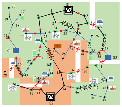 |  |  |
| Restoration stage 1 | 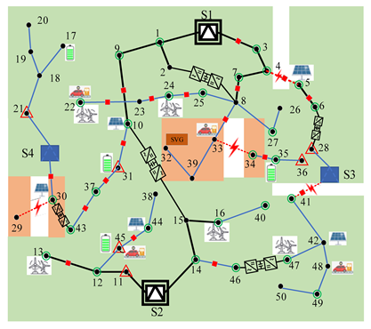 |  | 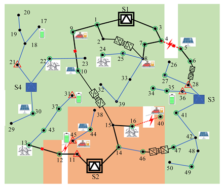 |
| Restoration stage 2 | 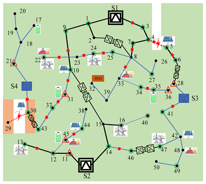 | 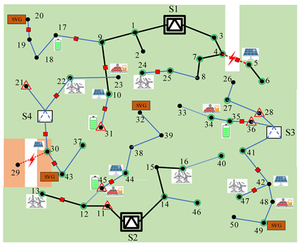 |  |
| Restoration stage 3 |  |  |  |
Disclaimer/Publisher’s Note: The statements, opinions and data contained in all publications are solely those of the individual author(s) and contributor(s) and not of MDPI and/or the editor(s). MDPI and/or the editor(s) disclaim responsibility for any injury to people or property resulting from any ideas, methods, instructions or products referred to in the content. |
© 2024 by the authors. Licensee MDPI, Basel, Switzerland. This article is an open access article distributed under the terms and conditions of the Creative Commons Attribution (CC BY) license (https://creativecommons.org/licenses/by/4.0/).
Share and Cite
Zhu, S.; Wang, P.; Lou, W.; Shen, S.; Liu, T.; Yang, S.; Xiang, S.; Yang, X. Resilience-Oriented Planning of Urban Distribution System Source–Network–Load–Storage in the Context of High-Penetrated Building-Integrated Resources. Buildings 2024, 14, 1197. https://doi.org/10.3390/buildings14051197
Zhu S, Wang P, Lou W, Shen S, Liu T, Yang S, Xiang S, Yang X. Resilience-Oriented Planning of Urban Distribution System Source–Network–Load–Storage in the Context of High-Penetrated Building-Integrated Resources. Buildings. 2024; 14(5):1197. https://doi.org/10.3390/buildings14051197
Chicago/Turabian StyleZhu, Sheng, Ping Wang, Wei Lou, Shilin Shen, Tongtong Liu, Shu Yang, Shizhe Xiang, and Xiaodong Yang. 2024. "Resilience-Oriented Planning of Urban Distribution System Source–Network–Load–Storage in the Context of High-Penetrated Building-Integrated Resources" Buildings 14, no. 5: 1197. https://doi.org/10.3390/buildings14051197