
Impact of Demand-Side Management on Thermal Comfort and Energy Costs in a Residential nZEB


1
Catalonia Institute for Energy Research (IREC), 08930 Sant Adrià de Besòs (Barcelona), Spain
2
Department of Automatic Control, Polytechnic University of Catalonia (UPC), 08028 Barcelona, Spain
3
Department of Fluid Mechanics, Polytechnic University of Catalonia (UPC), 08019 Barcelona, Spain
*
Author to whom correspondence should be addressed.
Buildings 2017, 7(2), 37; https://doi.org/10.3390/buildings7020037
Submission received: 31 March 2017
/
Revised: 28 April 2017
/
Accepted: 2 May 2017
/
Published: 9 May 2017
(This article belongs to the Special Issue Towards Decarbonization in the Building Sector: Innovating Net Zero Energy Buildings)
Abstract
:In this study, simulation work has been carried out to investigate the impact of a demand-side management control strategy in a residential nZEB. A refurbished apartment within a multi-family dwelling representative of Mediterranean building habits was chosen as a study case and modelled within a simulation framework. A flexibility strategy based on set-point modulation depending on the energy price was applied to the building. The impact of the control strategy on thermal comfort was studied in detail with several methods retrieved from the standards or other literature, differentiating the effects on day and night living zones. It revealed a slight decrease of comfort when implementing flexibility, although this was not prejudicial. In addition, the applied strategy caused a simultaneous increase of the electricity used for heating by up to 7% and a reduction of the corresponding energy costs by up to around 20%. The proposed control thereby constitutes a promising solution for shifting heating loads towards periods of lower prices and is able to provide benefits for both the user and the grid sides. Beyond that, the activation of energy flexibility in buildings (nZEB in the present case) will participate in a more successful integration of renewable energy sources (RES) in the energy mix.
1. Introduction
The urgently needed decarbonization of our energy systems will require an ever increasing proportion of energy coming from renewable sources (RES). The latest published Energy Strategy of the EU aims, for example, for a 27% share of RES in the energy consumption by 2030 [1]. Among those, solar and wind power have shown the most dynamical development over the last decade, their combined installed capacity having been multiplied by 10 between 2005 and 2015 [2]. While this rapid growth is a source of satisfaction for all the countries committed by the Paris Agreement to increase their share of RES [3], the variable nature of solar and wind power also poses certain threats to the stability of the electricity grids. Indeed, these two power sources highly depend on climatic conditions, which can result in possible mismatch between this variable production and the demand when the penetration of RES is high. To tackle these issues, demand-side management has been identified as a promising set of methods to help balance energy production and demand at any time [4,5]. In particular, buildings with embedded thermal mass (which can be used as thermal storage) represent great potential for energy flexibility [6], given that they already account for around 33% of the final energy consumption worldwide [2].
The trend for increasing the energy flexibility of the demand side will soon reach the building sector. The European Union already requires its member states to only construct nearly zero energy buildings (nZEB) by 2020, which means they should achieve a nearly annual zero energy balance [7]. In the future, buildings not only will need to be energy-efficient and reach the nZEB target, they will also have to be energy-flexible. In fact, buildings are becoming micro-energy hubs, including production units, storage, demand response possibilities, and flexible loads. Taking into account this evolution, the nZEB 2.0 of the future will be an interactive player in the energy grids and could even play an important role as such in the transformation of the European energy market [8].
However, to succeed in this transition towards smarter buildings, appropriate control strategies are required. The flexibility of heating or cooling loads can be controlled in different manners. The first group of methods consists of simple rule-based controls (RBC), which aim at avoiding peak periods with fixed schedules [9], reducing the peak power exchange between buildings and the grid [10], reducing the energy cost [11] or increasing the consumption of RES [12]. More advanced control strategies revolve around model predictive control (MPC), which consists of an optimization problem, most commonly used for decreasing the energy bills when variable electricity tariffs are applied [13,14,15]. However, the implementation of this second group of control strategies remains difficult due to the need of models (for the controller) and the high computation efforts [16]. In this paper, a rule-based control reacting to the electricity price is implemented and its impact is evaluated.
Furthermore, these control strategies often include comfort constraints in order to not let the flexibility objective jeopardize the satisfaction of the building’s occupants. For this reason, the evaluation of comfort (or discomfort) in such a scenario becomes even more crucial, since the flexibility control strategies will often aim at operating the building systems close to the boundaries. The present article thus proposes to compare different methodologies to evaluate the long-term comfort conditions of the occupants and to use them to check whether the implemented control strategy creates discomfort at some periods. In particular, the methods presented in ISO standard 7730 [17] and by Carlucci [18] are utilized. Special attention is drawn to the differences between the dayzone and the nightzone; the indoor temperature is lowered at night through a setback function, but it is supposed that comfort is still maintained when the occupants are sleeping. One objective of the paper therefore consists in studying how the different long-term comfort indices comprehend the comfort conditions at night.
In the present study, the first section details the utilized methods. Building simulation work was performed; therefore the different assumptions on the building characteristics, simulation boundaries, and implemented control are presented. Three methods are chosen for the evaluation of comfort; their calculation process is also detailed. In the Results section, thirteen study cases are analyzed in terms of comfort, flexibility, energy use and costs, and load cover factor. Finally, discussion and conclusions are drawn based on the observed results.
2. Materials and Methods
2.1. Building Study Case
2.1.1. Description of the Building and Its Occupancy
The dwelling used as a pilot site is representative of a multi-storey building typology of the period from 1991 to 2007 [19]. This typology is built under the Catalan building regulation NRE-AT-87 [20]. The building typology was analyzed previously [21] from the point of view of the energy efficiency renovation, considering the thermal comfort, the energy savings, and the economic evaluation. For this study, a deep refurbishment of the building has been considered in order to achieve a nearly zero energy building and implement flexible strategies.
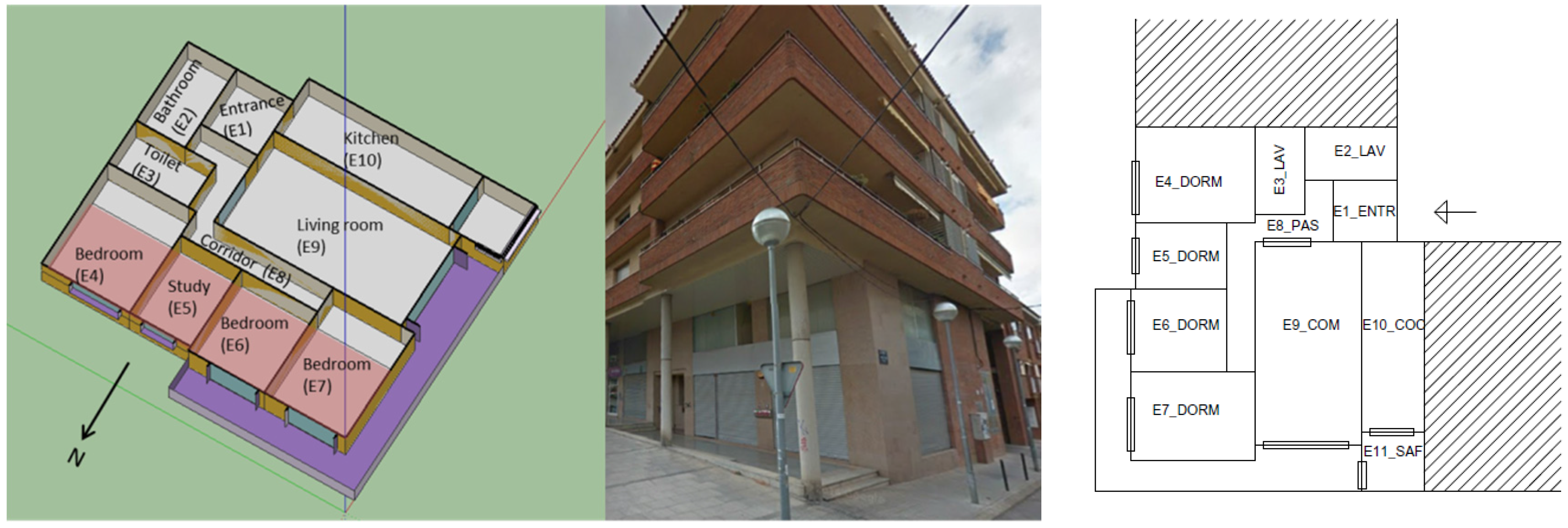
The dwelling is on the first floor of the building with two external façades oriented to the north and west, as Figure 1 shows. The building geometry is introduced in the simulation by a multizone 3D model, using the plugin TRNSYS3D for SketchUp. The flat is divided into actual rooms, and every room has been classified according to its use, including night and day zones. The building is modelled in TRNSYS, including the external environment and its corresponding shadings. The dwelling is occupied by a family with two adults and two children. Their occupancy profile has been adapted according to the habits of the family during a typical week (an example can be seen in Figure 5). Table 1 describes the building characteristics before and after the retrofit. More details about the building model hypothesis are described in [22,23].
2.1.2. Heating and DHW System
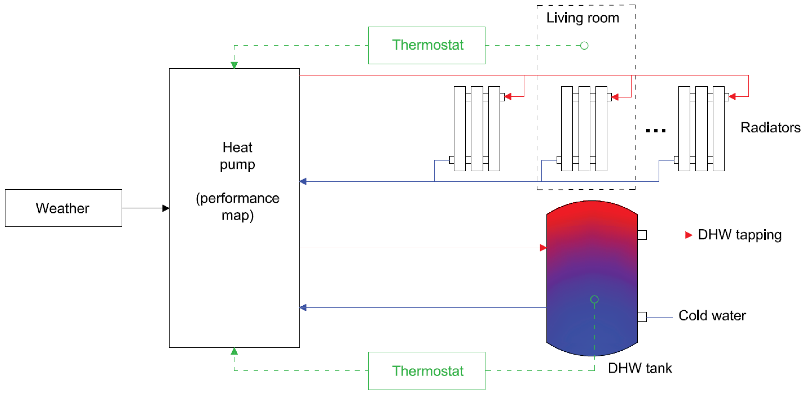
The hot water for space heating (SH) and Domestic Hot Water (DHW) is produced by an air-to-water heat pump, which is modelled by a performance map considering the water inlet temperature and the outside air temperature. In standard conditions (leaving water at 35 °C and outside air at 7 °C), the constructor of the modelled heat pump claims a COP of 5.25 [25]. The scheme of the heating system is presented in Figure 2.
Heating is provided in the indoor space by eight radiators (four in each zone). They are modelled as dynamic radiators, which means that once the water flow is stopped, the radiator continues to emit heat until the water it contains cools down. The heating power thus follows an exponential decay when the radiator stops, which is a more realistic behavior. The radiators’ flow is controlled by a unique thermostat placed in the living room and whose settings are further explained in Section 2.3; the water supply temperature is calculated with the heat pump performance map model.
DHW is stored in a water tank of 250 L, which is normally kept around 60 °C and has a heat loss coefficient of 0.75 W/m2·K. The DHW extractions follow the tapping programme No. 2 from standard EN 15316-1 [26]. When DHW is tapped, the heat pump is entirely dedicated to this task; therefore space heating is interrupted.
The electric consumption of the appliance stock has been obtained using the stochastic model described in [23].
2.1.3. PV System
A PV system is installed on the roof of the building to reduce the energy balance of the dwelling and reach the nZEB target. Ten modules of 140 Wp are installed, summing up to 1.4 kWp. The sizing was realized so that the PV system approximately provides half of the annual electrical energy consumption of the apartment (regardless of the concurrence between production and demand).
The percentage of the electrical load covered by on-site generation is analyzed using the load cover factor described in [27].
2.2. Comfort Criteria
As recalled in the introduction, the evaluation of comfort is an imperative aspect to take into account when designing control strategies that play with the indoor temperature set-points. Some indicators provide instantaneous evaluation of the general comfort conditions, such as the operative temperature, the PMV/PPD from Fanger [17], or percentages of people dissatisfied from various local thermal discomfort situations (asymmetry, vertical differences or draught for instance) [28]. Plotting their time series can provide a first comprehension of the comfort conditions indoors, but these indicators remain localized, both in space and time. For this reason, long-term indices are needed to evaluate comfort on larger time and space scales. These sorts of indicators provide a single value, or a set of a few values, that represent the comfort or discomfort conditions occurring over a certain time period and thus enable the comparison of different study cases in a more practical manner.
Three main different methods are used in the present study to calculate long-term comfort evaluation. The first two methods come from the standard EN 15251 (Annex F) [28], while the last one was retrieved from Carlucci [18]. All methods rely on the thermal comfort model developed in the 70s by Fanger; this model represents the thermal balance between the internal heat of the body and its thermal losses to the environment. The parameters that take part in this heat exchange are environmental parameters (air temperature, humidity, air velocity), human body parameters (heat generation and skin temperature and surface, among others), and clothing level. The three methods are described below and will later be compared with each other.
2.2.1. Method A: Percentage outside the Range
This method consists in calculating ‘the percentage of occupied hours when the PMV or operative temperature is outside a specified range’. To define the range, the different comfort categories as presented in Table 2 can be used, which correspond to different acceptation levels of PMV. The standard provides nominal values for residential buildings; however, it does not account for the changing conditions over night, when the occupants have a lower activity level and a higher clothing insulation (blanket for instance). For this reason, the temperature ranges were recalculated, differently for the day and night zones. The percentages in the ranges of Category I to IV can be represented as a ‘foot-print’ of the thermal environment.
In Method A1, the ranges from the standard are used (third column), and the monitored operative temperature is the one of the living room (where the thermostat is placed). In method A2, the calculated ranges for day and night zone (columns 4 and 5 from Table 2) are used instead of the constant ranges from the standard.
2.2.2. Method B: Degree Hours Criteria
In this method, ‘the time during which the operative temperature exceeds the specified range during the occupied hours is weighted by a factor depending on by how many degrees the range has been exceeded’. The calculation method is described in the standard [28] and results in a value which has the unit of hours. The ranges from the standard are used in method B1, and the calculated ranges for the day and night zones are used in method B2. For simplification and clarity issues, the results are only presented for Category II.
2.2.3. Method C: Long-Term Percentage of Dissatisfied (LPD)
This long-term index was developed by Carlucci [18]. LDP is a symmetric index that is able to evaluate the overheating and the overcooling of the building. It is normalized over the total number of people inside the household, over all the zones and over all the time corresponding to the calculation period (annual, warm or cold season). An advantage of the calculation period is to detect the weaknesses and strengths of the building. The LDP is calculated following Equation (1):
where is the counter of the time step of the calculation period, is the calculation period, is the counter for the zones of the household, is the total of zones of the household, is the zone occupation rate at certain time step, is the duration of a calculation time step, and is the Likelihood of Dissatisfied inside a certain zone (z) at a certain time step (t). The LD depends on the comfort model and is a function of the short-term index. In the present case, the LD is the PPD derived from Fanger’s model.
2.3. Control Strategy
The reference control strategy here consists in applying fixed set-points for the production of domestic hot water (DHW) and space heating (SH) by the heat pump. A set-point of 60 °C is maintained in the DHW tank to guarantee comfort and avoid the spread of legionella. For the room thermostat, the reference set-points for day and night are chosen based on the limits recommended for the different comfort categories, as presented in Table 2. The calculated operative temperature limits are represented with grey lines in Figure 3a. Given these limits and anticipating the set-point modulation implemented later, the reference set-points are fixed to 20.2 °C for daytime and 18.8 °C for nighttime or unoccupied periods. These values were chosen so that the set-point of the operative temperature stays within comfort Category II (normal level of expectation), even in cases of downwards set-point modulation, as shown in Figure 3b.
Starting from this reference, a control strategy aimed at improving the energy flexibility is implemented. It consists in modulating the reference heating set-points for DHW and SH, depending on the current price of electricity, and was partly inspired by [29].
Firstly, thresholds representing the limits of the high and low prices are defined. The data of the varying electricity price of the prior 24 h is collected. It is supposed that smart meters enable easy communication with the Distribution System Operator (DSO) and facilitate this data collection. In fact, the European Union plans to replace at least 80% of electricity meters with smart meters by 2020 wherever it is cost-effective to do so [30], and in Spain this deployment will even be implemented by 2018 [31]. The access to the varying electricity price profiles of the past day is therefore considered as given. These data are treated as follows: the 30th percentile of the distribution constitutes the threshold for low price and the 70th percentile constitutes the threshold for high price. The values of the percentiles have been selected based on a prior parametric analysis [32], which showed that the 30th and 70th percentiles give the best compromise between flexibility, comfort, and energy savings. At every time step, the calculation of and is repeated, and the current electricity price is compared with the thresholds; if it falls below , the set-point is increased to store thermal energy in the mass of the building while energy is cheap. If the current price is above , the set-point is decreased to discharge the stored thermal energy instead of using active systems while energy is expensive. To realize these variations, a modulation factor is introduced, as shown in Equation (2) and in Figure 4. The calculation of the SH and DHW temperature set-points is summarized in Equations (3) and (4). The amplitude of the modulation is for SH and for DHW, realized over the reference case aforementioned. It should be noted that the flexibility control strategy can be applied only to the SH set-point or for both the DHW and SH set-points at the same time. Overall, the strategy aims at shifting the loads towards periods with lower energy prices. The resulting set-point profile for room temperature is presented in Figure 3b.
To evaluate the impact of the strategy on load-shifting, a flexibility indicator is introduced [29]. It is calculated according to Equation (5), and the resulting value varies between −1 and 1, −1 meaning no energy was consumed during low-price hours and 1 meaning that no energy was consumed during high-price hours.
where is the electrical power of the heat pump, integrated over the lower or higher price periods defined with the 30th and 70th percentiles, as previously described.
2.4. Simulation Boundaries
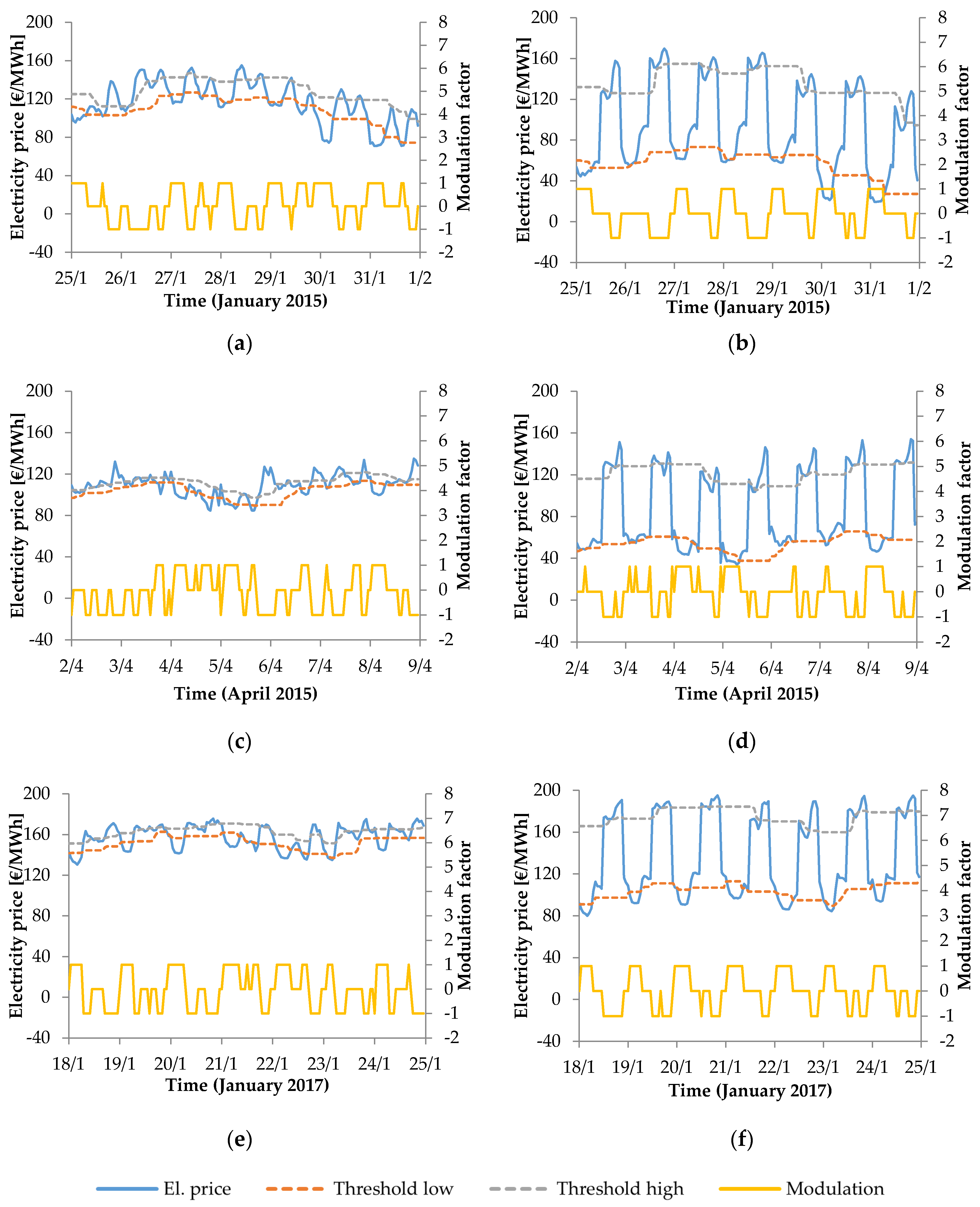
The pilot site is located in Terrassa (Barcelona, Spain) in a residential urban area. The weather data used for the simulation are retrieved from a weather station located in the city centre of Terrassa for 2015 and from another station situated in the centre of Barcelona for 2017. The price data used in the control strategy are retrieved from the Spanish Transmission System Operator (TSO) [33] and are synchronized with the corresponding weather data. The applied tariff corresponds to the active energy invoicing price, an hourly tariff implemented in Spain since 2014 for small consumers with a contracted power of less than 10 kW [34]. Two different tariffs exist; the default one, which varies hourly but in a limited range, and the two-period tariff, which includes larger variations between day and night. The price input for both tariffs is presented in Figure 4a,c,e for the default tariff and Figure 4b,d,f for the two-periods tariff. The two-period tariff presents higher potential for benefitting financially from the load-shifting, given its lower valleys and higher peaks. In fact, its standard deviation is significantly higher than the default tariff (38 to 44 €/MWh against 10 to 21 €/MWh for the default tariff).
The different cases simulated are presented in Table 3. Cases 1 to 6 test the different control strategies with the weather input from January 2015; the default tariff is used in Cases 1 to 3 and the two-period tariff in Cases 4 to 6. Given the higher potential of the two-period tariff, it is chosen for the remaining of the cases. Cases 7 to 9 carry out a similar analysis but in mid-season (April 2015), therefore with reduced space heating needs. These two periods were chosen since they are the most representative of different configurations within the heating season. Cases 10 to 12 test the robustness and repeatability of the control strategy with a different price and weather profile (taken from January 2017). Finally, Case 13 studies the influence of changing the amplitude of the set-point modulation; it is set to ±2 °C instead of ±1 °C, as in the other cases.
3. Results
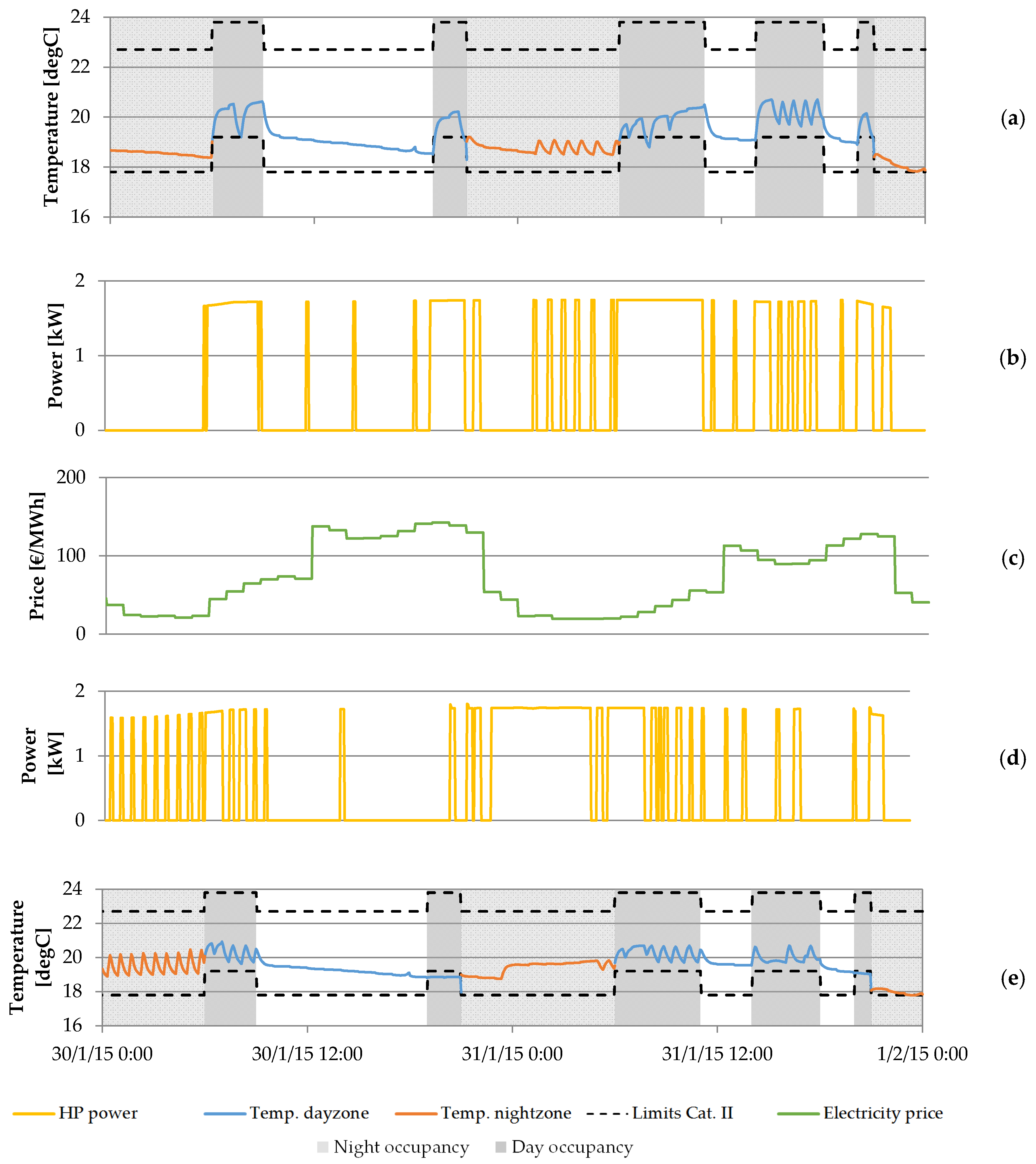
The results of the thirteen simulated cases are primarily obtained in the form of time series. A sample is presented in Figure 5 for Cases 4 and 6. The load shifting can be observed; the heat pump is operated more often during the valleys of the price profile and less often during the price peaks, when comparing Figure 5b,d. It can also be observed that the indoor temperature stays most of the time within the limits of Cat. II. The operative temperature is generally lower in the nightzone, notably due to the position of the bedrooms in the dwelling (more surfaces adjacent to the outside, resulting in higher heat losses). The time series give a first apprehension of the effects of the flexibility strategy, which will be quantified in detail using the proposed indicators in the following, Section 3.1, Section 3.2 and Section 3.3.
3.1. Comfort Evaluation
The impact of the rule-based control strategy on thermal comfort is investigated in detail, since increasing the flexibility of heating loads potentially induces risks of discomfort. The different study cases presented in Table 3 are analyzed using the methods of Section 2.2, resulting in the data of Table 4. Cases 2, 5, 8, and 11 respectively present very similar results to Cases 3, 6, 9, and 12, with regards to thermal comfort (the additional activation of the DHW tank barely affects the indoor environment). They are therefore not presented in Table 4. For all methods, the different zones are taken into account in the analysis only when they are occupied, hence the distinction of dayzone and nightzone for Methods A and B.
The first clear conclusion drawn from this table is the importance of differentiating the temperature ranges for day and night comfort evaluation. If one considers only the fixed ranges of the standards (method A1, equal for the day and nightzone), discomfort seems to occur in the night zone, as can be seen in Table 4. In fact, all the occupancy time of this zone is spent outside Category II for certain cases (1, 4, 7, and 10 notably). However, when one considers the different occupant behavior at night (lower metabolic rate and higher clothing insulation due to resting), the results then reveal a maintenance of the comfort level, despite the lower operative temperature observed. When using these adapted ranges (method A2, different for the day and the night zones), the comfort conditions in terms of PMV are very similar between the day and the night zone. Therefore, Methods A2 and B2 are preferred to Methods A1 and B1. From this point, these methods with the adapted ranges will be used when analyzing the comfort conditions.
Secondly, Table 4 presents a comparison of the different methods A, B, and C. Method A gives a fairly graphic overview of the comfort conditions, especially the repartition of the time spent in the different comfort categories. However, this analysis must be made separately for the day zone and the night zone, since the percentages are calculated at a single point. The differences between rooms can thus be observed. The results of Method B (degree hours) are consistent with those of Method A.
If Method A indicates how much time is spent outside a comfort range, it does not provide information about the gravity or amplitude of this violation, which is the purpose of Method B. However, the degree-hours criterion is more difficult to interpret when no point of comparison is available. In the present study, different cases are simulated, so the values of degree-hours can be compared across the cases, but Method B would not be suited to the analysis of a single case without prior reference of the degree-hours value (no threshold values are mentioned in the standards). In particular, the results depend on the duration of the simulation: the degree-hours are here presented for simulations of one week, but the order of magnitude of the results would completely change when simulating a whole year, for example.
Method C presents the advantage of lumping the comfort conditions into one single value, making possible a direct ranking between different study cases. For instance, comparing Cases 10 and 12 with Method B leads to the following analysis: from Case 10 to 12, the comfort is slightly degraded in the day zone (from 1.3 to 3.0 degree hours) and slightly improved in the night zone (from 6.1 to 4.7 degree hours). No clear conclusion can be drawn from this analysis, while the LPD reveals an overall higher discomfort in Case 12 (7.3%) than in Case 10 (6.5%). Method C therefore leads to a clearer distinction between the different cases, weighing the different rooms of the dwelling according to their occupancy. However, if a single room shows discomfort issues, this problem might not be revealed by the sole analysis of the LPD. For these reasons, it is recommended to utilize different methods in combination (Methods A2 and C, for example) when investigating flexibility scenarios and their impact on comfort, since they provide complementary information.
From Table 4, a generally slightly negative impact of energy flexibility on thermal comfort can be observed. To carry out this analysis, the flexibility cases 3, 6, 9, and 12 are compared with their respective reference cases 1, 4, 7, and 10. The LPD index increases from 0.1% to 0.8% when the flexibility control strategy is activated. However, the amplitude of this increased discomfort is rather minimal, and the comfort conditions are maintained, with a LPD well below the limit of 10%. In January 2015, the flexibility has a rather low impact (LPD increased of only +0.1%) with the default tariff, while it is more pronounced with the two-period tariff (+0.3%). In April 2015, the LPD also increases by 0.3%, but the general comfort is better than in winter: the degree-hours criterion is null and all the occupancy time is spent within Category II. January 2017 presents the worst increase of LPD (+0.8%) and the highest discomfort, due to colder outdoor temperatures during this period.
Furthermore, it can be seen from the graphs of Method A that the time spent in both Categories I and III is increased for the flexibility cases. This expresses the variations due to the set-point modulations; more time is spent with improved comfort but also more time with degraded comfort. Finally, it should be noted that the flexibility strategy generally improves comfort in the night zone but degrades it in the day zone. This effect is due to the profile of the electricity price; energy is generally cheaper at night, which triggers an upwards set-point modulation from the control strategy, hence a comfort improvement, and acts reversely during daytime.
The last lesson learnt from the comfort evaluation relates to Case 13, in which a higher modulation of the indoor set-point was implemented (±2 °C instead of ±1 °C). This strategy provokes higher amplitude of the indoor temperature variations, leading to higher discomfort; the LPD changes from 6.8% to 9.4% from reference Case 4 to Case 13. Furthermore, 4.4% of the occupancy time is then spent in Comfort Category IV, while there was no time spent in this category in the corresponding reference case. Based on these conclusions, it is recommended not to exceed a modulation of ±1 °C in the set-point when activating energy flexibility indoors.
3.2. Energy Flexibility Evaluation
The different study cases are analyzed in terms of energy flexibility in Figure 6. It can first be observed that the reference cases 1, 4, 7, and 10 all have a neutral or negative flexibility factor. This reveals that the dwelling normally uses more electricity at times of higher prices than at times of lower prices. It is particularly true for DHW consumption, with flexibility factors always lower than −0.5 when no specific strategy is implemented, thus leaving room for improvements.
The positive impact of the proposed flexibility rule-based control is visible on all the cases in which it is implemented. In January 2015, the total flexibility factor of the heat pump is increased from −0.11 to 0.76 (default tariff) or from −0.28 to 0.70 (2-periods tariff); in April 2015 it is increased from −0.28 to 0.63 and in January 2017 from −0.17 to 0.75. Overall, the strategy functions well and enables an important part of energy use to be shifted towards periods with lower electricity prices.
In spring season (April 2015, cases 7, 8, and 9), the demand for space heating is lower and thus more flexible. For this reason, the entire heat pump operation for space heating can be shifted to low-price hours, resulting in the maximum value of the SH flexibility factor being equal to 1 in Cases 8 and 9. For DHW, the flexibility factor starts at a very low value in the reference cases and therefore cannot reach the maximum of 1. A fraction of the demand cannot be shifted, despite the flexibility control strategy implemented and the storage tank. The demand for DHW is nearly constant throughout the year, so no clear difference is visible between the spring and winter cases.
Overall, the additional flexibility provided by DHW has a low impact on the total HP flexibility factor in the winter cases. For instance from Case 2 to Case 3, the HP flexibility factor is further improved only from 0.62 to 0.76; from Case 5 to Case 6, it is improved from 0.59 to 0.70; and from Case 11 to Case 12, it is improved from 0.64 to 0.75. The low impact of DHW flexibility is due to the relative importance of the DHW needs compared to space heating in winter. On the other hand in spring season, the additional flexibility provided by DHW improves the flexibility factor from 0.30 to 0.63. This more important increase is due to the larger relative importance of DHW needs in mid-season.
3.3. Impact on Energy Use, Operational Costs and Load Cover Factor
The energy use, associated costs, and load cover factor for every studied case are summarized in Table 5. Two values of heat pump electricity use are presented: the total consumption, and the electricity needed from the grid (i.e. after subtracting the available electricity production from the PV panels). The same trend can be observed in most sets of cases; the flexibility control strategy leads to a reduction of the operational costs while increasing the electricity use. This latter effect is attributable to what can be identified as ‘storage losses’; heat is stored in the thermal mass of the building (or the DHW tank) during low-price periods for use later on when the price decreases. Like any form of storage, energy losses thus occur. In the studied cases, the electricity use of the heat pump is increased by 3% to 12%.
When examining the last week of January 2015 (Cases 1 to 6), it can be observed that the two-period tariff amplifies the effects of the control strategy, compared with the default tariff. In fact, even without any flexibility control, the energy costs are already reduced by 16% (between Cases 1 and 4) by choosing the two-period tariff over the default one. With the default tariff and the flexibility control, the heat pump energy use is increased by up to 7.3% and the associated costs are stable (slight increase of up to 1.3%). The two-period tariff enables the cost saving to actually be realized further (−21.4%), although with an electricity use increased by 9.7%. As anticipated, the lower valleys in the price profiles of the two-period tariff enable larger savings when energy is shifted to these low-price periods.
Case 13 (with higher amplitude of the set-point modulation) also amplifies the effect of the control strategy. The cost savings reach 21.9%; hence they are not substantially more than in Case 6. However, the amount of electricity spent increases by 12.4%, which could start to affect negatively the nZEB energy balance targeted by this building. Taking also into account the impact on thermal comfort already discussed, it is advised to avoid modulations of ±2 °C in the indoor temperature set-point.
Cases 6 and 12 can be compared to analyze the performance of the strategy in similar conditions (winter season) but in different years. The flexibility scenario in January 2017 is less efficient, with cost savings of 16% compared to 21.4% in 2015 for the energy spent in operating the heat pump. The electricity price range used in Cases 10 to 12 in 2017 (from 80 to 190 €/MWh) was considerably higher than in Cases 4 to 6 in 2015 (from 30 to 160 €/MW·h), leaving less room for monetary savings. This situation was due to higher stress on the national electricity markets in January 2017.
Case 9 presents the highest increase in grid electricity use among the cases, with a ±1 °C set-point modulation (+10.3%). This case is simulated in spring season, with the heat pump only operating punctually for space heating. The upwards modulation of the set-point thus forces the heat pump to operate, storing energy in the thermal mass of the building although it is not necessarily needed afterwards and leading to higher storage losses. The use of upwards modulation should therefore be used with care in the context of mid-season and reduced heating loads.
The chosen flexibility control strategy also impacts the load cover factor, as can be seen in Table 6. This indicator gives information on how much of the energy consumed by the building is covered by the local PV. The proposed price-based strategy generally tends to move the operation of the heat pump towards periods of lower prices, which usually occur at night, when the PV production is inexistent. This effect is visible on the load cover factor; when implementing the flexibility strategy, this indicator decreases by 2% to 3%. This impact is not negligible, but overall the effect of the flexibility strategy on the self-consumption of the building is limited.
4. Discussion
When analyzing the simulation results in terms of comfort, the threshold ranges in temperature for the different comfort categories have been lowered for the night zone. This process is backed by serious assumptions concerning the occupants’ behavior at night (lower metabolic rate and higher clothing insulation) and the space heating habits in Mediterranean countries. The indoor set-point always stays within the recommended limits for health [35]. However, adapting the comfort temperature ranges should always be realized with care since it will incite the control strategy to operate the systems at lower temperatures at night, closer to the boundaries. Even though it was demonstrated that thermal comfort is still maintained in terms of PMV under the considered assumptions, several local discomfort situations might occur. These local discomforts were not accounted for the present work since the simulation tools do not allow such detailed analysis. They include, for instance, draught risk, vertical air temperature differences or radiant temperature asymmetry [36], parameters which could become more critical if the air temperature is already lowered. Further analysis should be carried out to guarantee the absence of such localized discomfort situations when the indoor temperature set-point is lowered for energy flexibility purposes. However, it is expected that such issues would not occur, especially in a nZEB with high insulation levels.
The present work has compared different methods to evaluate long-term thermal comfort (over periods of one week in this case). The percentages within the ranges (Method A) provide a graphic overview of the occupancy time within the different comfort categories. The degree-hour criterion (Method B) provides insights on the amplitude of the comfort boundaries violations, but can only be calculated for a single comfort category (Cat. II presented here). These two methods are computed at a single measurement point; therefore they only give indications of the comfort at that particular location. Method C averages the percentage of people dissatisfied (PPD) in the different rooms when they are occupied and thus results in a single output value for the whole building. This indicator is therefore convenient for the comparison of different cases or different buildings, and it is advised to utilize it when carrying out thermal comfort analysis after the implementation of energy flexibility strategies. If a more detailed analysis is required to understand the comfort discrepancies between different rooms, then Methods A or B might represent more suitable tools. A combination of different methods is always in order to obtain a detailed analysis.
Analyzing the results of the flexibility scenarios enables the formulation of different recommendations with regards to a foreseen implementation, especially in the context of Mediterranean countries. Firstly, it was shown that contracting the hourly ‘two-periods’ tariff enables cost savings thanks to the flexibility control strategy, which was not the case with the default tariff. The two-period profile presents larger daily variations, which makes more profitable the load-shifting towards low-price periods. Secondly, a set-point modulation of ±2 °C was tested; it resulted in similar cost savings and flexibility but also in increased electricity use and the appearance of several discomfort situations. It is thus advised to keep the indoor set-point modulation within a ±1 °C boundary. Thirdly, the results of the simulation carried out in Spring revealed that the upwards set-point modulation should be used with care when the heat pump operation is sparse: the heat stored during low-price periods can be entirely dissipated through losses before it is needed later on during high-price periods. Finally, nZEBs present an interesting potential for flexibility due to their reduced heating needs, even though the magnitude of the displaced energy use is lower. These conclusions should be taken into account when considering larger implementations of energy flexibility in residential buildings in Spain or the Mediterranean area.
It is important to analyze the final objective of the implemented energy flexibility. The presented control strategy is strictly aiming to reduce the operational energy costs of the dwelling through load shifting. As was previously mentioned, the adopted strategy also has side effects and notably a non-negligible increase in the electricity consumption. This could be seen as contradictory when a nZEB intends to lower its energy consumption as much as possible. However, with the overall picture in mind, the control strategy could enable the integration of more RES in the energy mix, which participates in the global goal of the decarbonization of our energy systems. The nZEB of the future might emphasize and reward energy flexibility more than the strict reduction of its demand since it will benefit the whole grid [8,37]. A slight increase in the energy consumption of buildings due to storage losses could be a ‘necessary evil’ in order to enhance the demand-side flexibility and thus achieve the shares of RES targeted by the national regulations.
An nZEB can play an important role in this regard. This type of building generally presents higher insulation levels than do standard constructions. As a result, the embedded thermal mass is able to retain heat for longer periods, leading to higher flexibility, even though the shifted loads have a lower amplitude (hence also less interest for the grid side) [29,38]. In this paper, the proposed control strategy has demonstrated that efficient load shifting is possible when applying a time-varying price structure. If this price profile is designed in a smart manner, the periods of cheaper energy price could coincide with periods of high production of RES, for instance [39]. In this way, the goal of cost savings would go along with an improvement in RES consumption. Along the same lines, Klein et al. [40] propose to utilize the residual load at the national scale as an input signal to activate the energy flexibility; these data could, for example, be used to design a price profile, applied in combination with the control strategy presented here. Similar methods could be developed to increase the consumption of on-site RES (such as local PV production). This would present different challenges since the on-site production currently does not coincide with periods of cheaper energy prices, as was shown with the load cover factor analysis.
5. Conclusions
In the present work, a flexibility control strategy was implemented in a Mediterranean nZEB and analyzed through simulation studies. The rule-based control reacts on thresholds of the electricity price, adjusting the temperature set-point indoors or in the DHW tank, depending on the current cost of electricity. This control strategy is easy to implement and logically leads to monetary savings of up to around 20% (on the energy purchased to operate the heat pump) in the studied periods. These savings are realized through the shifting of the heat pump operation towards periods of lower prices, hence storing energy in the thermal mass of the building or in the DHW water tank. This process also results in storage losses and an increase in the electricity consumption of up to 7%. The impact on thermal comfort is generally limited, even though the set-point modulation generally causes an increase of the LPD by 0.3% to 0.8%. The heat pump flexibility factor, which quantifies the load-shifting, is improved by around 0.9 in the studied cases. The control strategy also leads to a reduction of the load cover factor by 2% to 3%. The results obtained in Winter 2015 are globally consistent with the ones obtained in Winter 2017, which reveals the robustness of the adopted control and its usability in different contexts.
From these conclusions, it can be observed that the proposed control strategy affects several aspects of the dwelling operation and use; comfort, flexibility, energy cost, energy use, and load cover factor. Some of these parameters benefit the user (comfort, costs), while the others affect the grid side or the energy provider (energy use, flexibility). These features cannot all be improved at the same time since they can be conflicting. For instance, improving energy flexibility results in a degradation of the load cover factor. In fact, the energy loads are shifted to periods of cheaper energy prices, which mostly occur at night, when the PVs cannot cover the demand. Energy flexibility should thus always consist of a trade-off between those different aspects in order to create a situation that is beneficial for both parties. Designers of control strategies for improving the demand-side flexibility should keep this rule in mind to foster user acceptance and sustainable business models.
Further work includes the development of optimal control strategies and not only rule-based controls. Notably, Model Predictive Control (MPC) can deal with several weighted objectives and optimize the operation of a heating system considering information on the predicted future price or weather. In this way, the problem of balancing the energy use increase versus the cost savings could be managed in an optimal manner. The aggregation potential of flexibility should also be studied, since one building or nZEB has only a low impact alone but a larger cluster can provide more interesting features for the grid.
Acknowledgments
This project has received funding from the European Union’s Horizon 2020 research and innovation programme under the Marie Skłodowska-Curie grant agreement No 675318 (INCITE). Part of this work stems from the activities carried out in the framework of the IEA-EBC Annex 67 (International Energy Agency – Energy in Buildings and Communities program) about Energy Flexibility in Buildings.
Author Contributions
Joana Ortiz developed the building simulation model and participated in the data analysis; Jaume Salom supervised the work and contributed to the analysis of energy flexibility; Thibault Q. Péan run the simulations, analyzed the data and wrote the paper.
Conflicts of Interest
The authors declare no conflict of interest.
Nomenclature
| Abbreviations | Subscripts | ||
| COP | Coefficient of Performance | High-price periods | |
| DHW | Domestic Hot Water | Low-price periods | |
| DSO/TSO | Distribution/Transmission System Operator | Set-point | |
| LDP | Long-term of Dissatisfied Percentage | Time step | |
| MPC | Model Predictive Control | Building zone | |
| nZEB | Nearly-Zero Energy Building | Symbols | |
| PMV | Predicted Mean Vote | Electricity price | |
| PPD | Percentage of People Dissatisfied | Duration of time step | |
| PV | Photovoltaic | Likelihood Dissatisfied | |
| PVPC | Voluntary Price for Small Consumers | Modulation factor | |
| RBC | Rule-based control | Zone occupation rate | |
| RES | Renewable Energy Sources | Electrical power | |
| SH | Space Heating | Zone temperature | |
| Temperature modulation | |||
| Z | Total number of zones | ||
References
- European Commission. A Policy Framework for Climate and Energy in the Period from 2020 to 2030; Communication from the Commission to the European Parliament, the Council, the European Economic and Social Committee and the Committee of the Regions; European Commission: Brussels, Belgium, 2014. [Google Scholar]
- Renewable Energy Policy Network for the 21th Century (REN 21). Renewables 2016 Global Status Report; REN21 Secretariat: Paris, France, 2016. [Google Scholar]
- United Nations Framework Convention on Climate Change (UNFCC) Conference of the Parties (COP). Adoption of the Paris Agreement. Proposal by the President; FCCC/CP/2015/L.9/Rev.1; United Nations Office at Geneva: Geneva, Switzerland, 2015. [Google Scholar]
- The Power to Choose: Demand Response in Liberalised Electricity Markets; International Energy Agency: Paris, France, 2003; p. 156.
- Morch, A.; Wolfang, O. Post-2020 Framework for a Liberalised Electricity Market with a Large Share of Renewable Energy Sources; Market 4 RES; Intelligent Energy Europe: Trondheim, Norway, 2016. [Google Scholar]
- Conclusions and Recommendations—Demand Flexibility in Households and Buildings; IEA DSM Task 17; IEA: Paris, France, 2016.
- European Commission. Directive 2010/31/EU of the European Parliament and of the Council of 19 May 2010 on the energy performance of buildings (recast). Off. J. Eur. Communities 2010, L153, 13–35. [Google Scholar]
- D’Angiolella, R.; de Groote, M.; Fabbri, M. NZEB 2.0: Interactive players in an evolving energy system. REHVA J. 2016, 53, 52–55. [Google Scholar]
- Carvalho, A.D.; Moura, P.; Vaz, G.C.; de Almeida, A.T. Ground source heat pumps as high efficient solutions for building space conditioning and for integration in smart grids. Energy Convers. Manag. 2015, 103, 991–1007. [Google Scholar] [CrossRef]
- Dar, U.I.; Sartori, I.; Georges, L.; Novakovic, V. Advanced control of heat pumps for improved flexibility of Net-ZEB towards the grid. Energy Build. 2014, 69, 74–84. [Google Scholar] [CrossRef]
- Schibuola, L.; Scarpa, M.; Tambani, C. Demand response management by means of heat pumps controlled via real time pricing. Energy Build. 2015, 90, 15–28. [Google Scholar] [CrossRef]
- De Coninck, R.; Baetens, R.; Saelens, D.; Woyte, A.; Helsen, L. Rule-based demand-side management of domestic hot water production with heat pumps in zero energy neighbourhoods. J. Build. Perform. Simul. 2014, 7, 271–288. [Google Scholar] [CrossRef]
- Masy, G.; Georges, E.; Verhelst, C.; Lemort, V. Smart grid energy flexible buildings through the use of heat pumps and building thermal mass as energy storage in the Belgian context. Sci. Technol. Built Environ. 2015, 4731, 800–811. [Google Scholar] [CrossRef]
- Halvgaard, R.; Poulsen, N.K.; Madsen, H.; Jorgensen, J.B. Economic Model Predictive Control for building climate control in a Smart Grid. In Proceedings of the 2012 IEEE PES Innovative Smart Grid Technologies (ISGT), Washington, DC, USA, 16–20 January 2012; pp. 1–6. [Google Scholar]
- Ma, J.; Qin, S.J.; Salsbury, T. Application of economic MPC to the energy and demand minimization of a commercial building. J. Process Control 2014, 24, 1282–1291. [Google Scholar] [CrossRef]
- De Coninck, R.; Magnusson, F.; Åkesson, J.; Helsen, L. Toolbox for development and validation of grey-box building models for forecasting and control. J. Build. Perform. Simul. 2015, 9, 1–16. [Google Scholar] [CrossRef]
- International Organization for Standardization. UNE ISO 7730: Ergonomics of the Thermal Environment—Analytical Determination and Interpretation of Thermal Comfort Using Calculation of the PMV and PPD Indices and Local Thermal Comfort Criteria; IOS: Geneva, Switzerland, 2006. [Google Scholar]
- Carlucci, S. Thermal Comfort Assessment of Buildings; Briefs in Applied Sciences and Technology; Springer: Milan, Italy, 2013. [Google Scholar]
- Institut Català d’Energia. Rehabilitació Energètica D’edificis, Col·lecció Quadern Pràctic N° 10; Institut Català d’Energia: Barcelona, Spain, 2016. [Google Scholar]
- Normativa d’Aïllament Tèrmic d’Edificis; NRE-AT-87; Generalitat de Catalunya: Barcelona, Spain, 1987.
- Ortiz, J.; Fonseca, A.; Salom, J.; Garrido, N.; Fonseca, P.; Russo, V. Cost-effective analysis for selecting energy efficiency measures for refurbishment of residential buildings in Catalonia. Energy Build. 2016, 128, 442–457. [Google Scholar] [CrossRef]
- Ortiz, J.; Fonseca, A.; Salom, J.; Garrido, N.; Fonseca, P.; Russo, V. Comfort and economic criteria for selecting passive measures for the energy refurbishment of residential buildings in Catalonia. Energy Build. 2016, 110, 195–210. [Google Scholar] [CrossRef]
- Ortiz, J.; Guarino, F.; Salom, J.; Corchero, C.; Cellura, M. Stochastic model for electrical loads in Mediterranean residential buildings: Validation and applications. Energy Build. 2014, 80, 23–36. [Google Scholar] [CrossRef]
- Ventilation for Buildings—Calculation Methods for the Determination of Air Flow Rates in Buildings Including Infiltration; EN 15242; European Committee for Standardization: Brussels, Belgium, 2007.
- Hitachi Air Conditioning Products Europe. Technical Catalogue; Yutaki Series; Hitachi Air Conditioning Products Europe SAU: Vacarisses (Barcelona), Spain, 2016. [Google Scholar]
- Heating Systems in Buildings—Method for Calculation of System Energy Requirements and System Efficiencies—Part 3–1 Domestic Hot Water Systems, Characterisation of Needs (Tapping Requirements); EN 15316-1; European Committee for Standardization: Brussels, Belgium, 2007; pp. 1–20.
- Salom, J.; Marszal, A.J.; Widén, J.; Candanedo, J.; Lindberg, K.B. Analysis of load match and grid interaction indicators in net zero energy buildings with simulated and monitored data. Appl. Energy 2014, 136, 119–131. [Google Scholar] [CrossRef]
- Indoor Environmental Input Parameters for Design and Assessment of Energy Performance of Buildings Addressing Indoor Air Quality, Thermal Environment, Lighting and Acoustics; EN 15251; European Committee for Standardization: Brussels, Belgium, 2007.
- Le Dréau, J.; Heiselberg, P. Energy flexibility of residential buildings using short term heat storage in the thermal mass. Energy 2016, 111, 1–5. [Google Scholar] [CrossRef]
- European Parliament. Directive 2009/72/EC of the European Parliament and of the Council of 13 July 2009 Concerning Common Rules for the Internal Market in Electricity; European Parliament: Strasbourg, France, 2009. [Google Scholar]
- Real Decreto 1110/2007, de 24 de Agosto, por el que se Aprueba el Reglamento Unificado de Puntos de Medida del Sistema Eléctrico; Ministerio de Industria, Turismo y Comercio: Madrid, Spain, 2007.
- Péan, T.Q.; Ortiz, J.; Salom, J. Potential and optimization of a price-based control strategy for improving energy flexibility in Mediterranean buildings. In Proceedings of the CISBAT 2017 International Conference—Future Buildings and Districts—Energy Efficiency from Nano to Urban Scale, Lausanne, Switzerland, 6–8 September 2017. under review. [Google Scholar]
- Red Electrica de España ESIOS—Sistema de Información del Operador del Sistema. Available online: https://www.esios.ree.es/en (accessed on 4 April 2017).
- Gobierno de España. Ministerio de Industria Energía y Turismo Real Decreto 216/2014, de 28 de marzo, por el que se establece la metodología de cálculo de los precios voluntarios para el pequeño consumidor de energía eléctrica y su régimen jurídico de contratación. Boletín Oficial Estado 2014, 77, 27397–27428. [Google Scholar]
- World Health Organization. Health Impact of Low Indoor Temperatures; WHO Regional Office for Europe: Copenhagen, Denmark, 1987. [Google Scholar]
- Olesen, B.W. Indoor Environmental Input Parameters for the Design and Assessment of Energy Performance of Buildings. REHVA J. 2015, 52, 17–23. [Google Scholar]
- Mlecnik, E. Goodbye Passive House, Hello Energy Flexible Building? In Proceedings of the PLEA 2016 36th International Conference on Passive and Low Energy Architecture, Los Angeles, CA, USA, 11–13 July 2016. [Google Scholar]
- Reynders, G.; Nuytten, T.; Saelens, D. Potential of structural thermal mass for demand-side management in dwellings. Build. Environ. 2013, 64, 187–199. [Google Scholar] [CrossRef]
- Miara, M.; Günther, D.; Leitner, Z.L.; Wapler, J. Simulation of an Air-to-Water Heat Pump System to Evaluate the Impact of Demand-Side-Management Measures on Efficiency and Load-Shifting Potential. Energy Technol. 2014, 2, 90–99. [Google Scholar] [CrossRef]
- Klein, K.; Killinger, S.; Fischer, D.; Streuling, C.; Salom, J.; Cubi, E. Comparison of the future residual load in fifteen countries and requirements to grid-supportive building operation. In Proceedings of the 11th EuroSun Conference, Palma, Spain, 11–14 October 2016; pp. 11–14. [Google Scholar]
Figure 1.
3D model, photo, and floor plan of the study case building.

Figure 2.
Schematic view of the heating system.

Figure 3.
Limits of the comfort categories and room set-point profiles for (a) reference case; (b) modulated case.
Figure 3.
Limits of the comfort categories and room set-point profiles for (a) reference case; (b) modulated case.
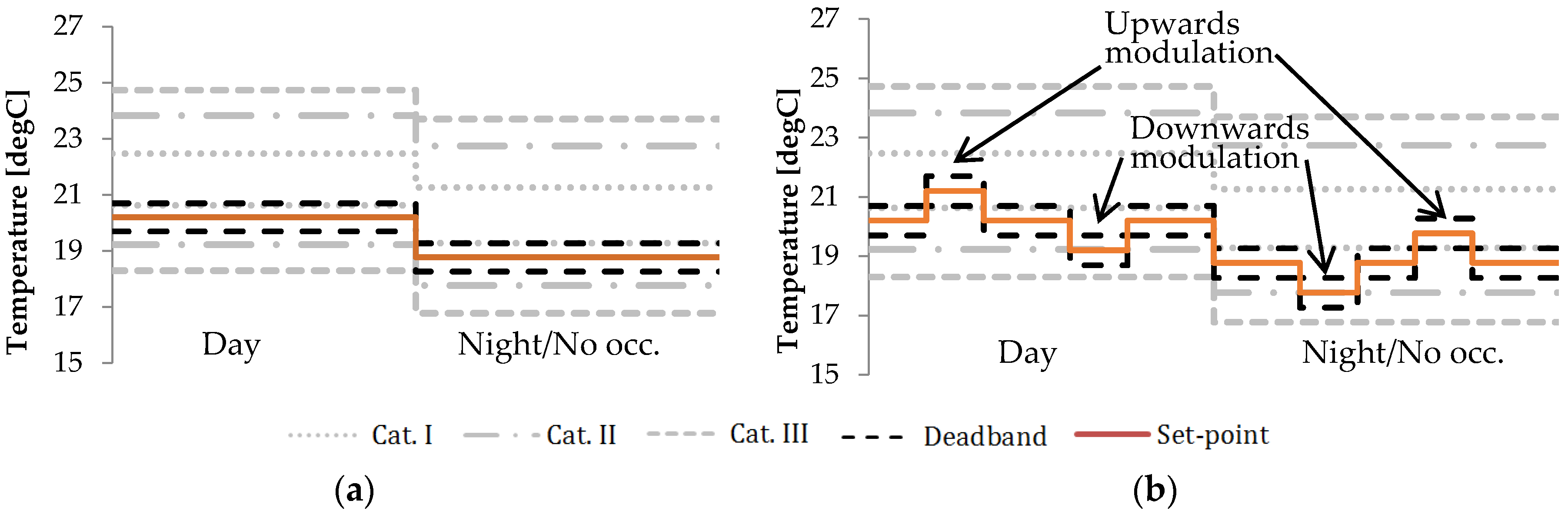
Figure 4.
Electricity price for end-users contracted on the PVPC tariff [33] in Spain in January 2015 for graphs (a,b); April 2015 for graphs (c,d); and January 2017 for graphs (e,f). On graphs (a,c,e), the default tariff is shown, while on graphs (b,d,f), the two-periods tariff is shown. The yellow curves show the modulation factor , equal to −1 in the case of a high price, to 1 in the case of a low price, and equal to 0 otherwise. This factor is multiplied afterwards by the amplitude to obtain the final set-point modulation (see Equations (3) and (4)).

Figure 5.
Example of results in the form of time series for two selected days. Graphs (a,b) respectively present the indoor temperature and the heat pump power for Case 4 (reference); Graph (c) shows the common electricity price for Cases 4 and 6 for 30 January 2015 and 31 January 2015 (two-periods tariff); Graphs (d,e) respectively present the heat pump power and the indoor temperature for Case 6 (flexibility case); In Graphs (a,e), the temperature curve is shown according to the occupancy; when the occupants are present in the dayzone (dark grey areas), the temperature of the living room is shown (in blue), while, when they occupy the nightzone (light gray areas), the temperature of one bedroom is shown (in orange). When the occupants are not present (white background), the temperature of the living room is shown.

Figure 6.
Flexibility factor analysis. Domestic Hot Water (DHW) refers to the flexibility factor computed using the heat pump power for the production of DHW. Space heating (SH) refers to the flexibility factor computed using the heat pump power for space heating. HP refers to the flexibility factor computed using the total heat pump power (DHW and SH).
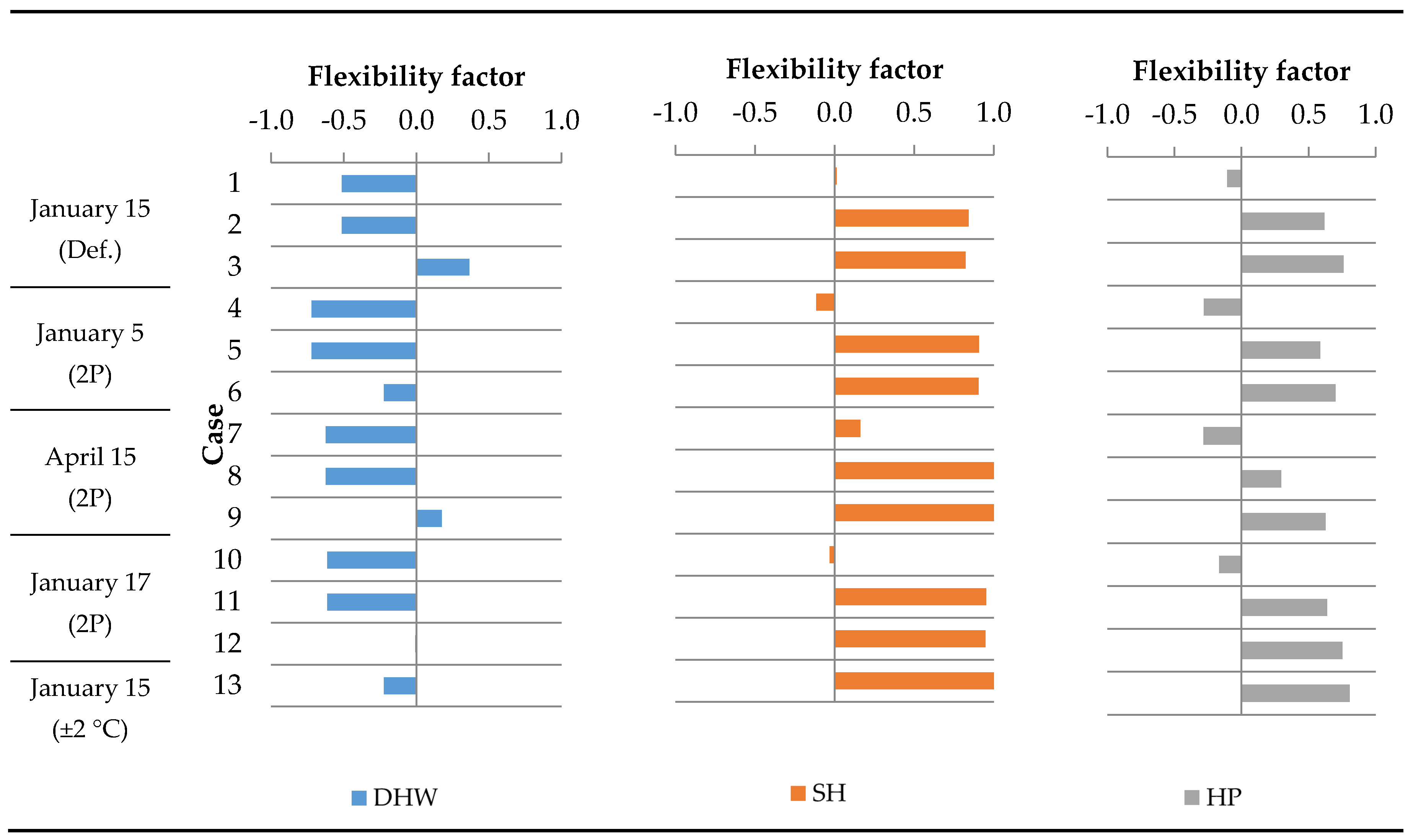

Table 1.
Main characteristics of the building before and after the retrofit.
| Parameter | Unit | Before Retrofit | After Retrofit |
|---|---|---|---|
| Location | - | Spain | |
| Building date | - | 1991–2007 | |
| Floor area | m2 | 108.5 | |
| Window area | m2 | 19.6 | |
| Protected volume | m3 | 263.6 | |
| U-value walls | W/m2·K | 0.6 | 0.2 |
| U-value windows | W/m2·K | 2.5 to 5.7 | |
| g-value windows | - | 0.5 to 0.76 | |
| Infiltration n50 [24] | h−1 | 7.5 | 5.0 |
| Heating and DHW | Natural gas boiler (η = 0.75) | Heat Pump | |
| Lighting system | Fluorescent | LED | |
| PV system | kWp | - | 1.4 |
Table 2.
Operative temperature ranges for the different categories. For the calculations, the following assumptions are taken: 1.2 met, 1 clo, 0.1 m/s for the day range and 0.8 met, 2.5 clo, 0.1 m/s for the night range.
Table 2.
Operative temperature ranges for the different categories. For the calculations, the following assumptions are taken: 1.2 met, 1 clo, 0.1 m/s for the day range and 0.8 met, 2.5 clo, 0.1 m/s for the night range.
| Category | PMV | PPD | Operative Temperature Ranges (°C) | ||
|---|---|---|---|---|---|
| EN 15251 for Residential | Own Calculation | ||||
| Day Range | Night Range | ||||
| Cat. I | |PMV| < 0.2 | PPD < 6% | 21–25 | 20.6–22.5 | 19.3–21.3 |
| Cat. II | |PMV| < 0.5 | PPD < 10% | 20–25 | 19.2–23.8 | 17.8–22.7 |
| Cat. III | |PMV| < 0.7 | PPD < 15% | 18–25 | 18.3–24.7 | 16.8–23.7 |
| Cat. IV | |PMV| > 0.7 | PPD > 15% | <18 and >25 | <18.3 and >24.7 | <16.8 and >23.7 |
Table 3.
List of simulation cases.
| Case | Weather Input | Price Tariff | Flexibility Control Strategy (Set-Point Modulation) | Modulation Amplitude | |
|---|---|---|---|---|---|
| 1 | January 2015 | Default | Reference (m = 0) | 0 | 0 |
| 2 | January 2015 | Default | Flexibility on SH | 1 | 0 |
| 3 | January 2015 | Default | Flexibility on SH + DHW | 1 | 5 |
| 4 | January 2015 | 2-periods | Reference (m = 0) | 0 | 0 |
| 5 | January 2015 | 2-periods | Flexibility on SH | 1 | 0 |
| 6 | January 2015 | 2-periods | Flexibility on SH + DHW | 1 | 5 |
| 7 | April 2015 | 2-periods | Reference (m = 0) | 0 | 0 |
| 8 | April 2015 | 2-periods | Flexibility on SH | 1 | 0 |
| 9 | April 2015 | 2-periods | Flexibility on SH + DHW | 1 | 5 |
| 10 | January 2017 | 2-periods | Reference (m = 0) | 0 | 0 |
| 11 | January 2017 | 2-periods | Flexibility on SH | 1 | 0 |
| 12 | January 2017 | 2-periods | Flexibility on SH + DHW | 1 | 5 |
| 13 | January 2015 | 2-periods | Flexibility on SH + DHW | 2 | 5 |
Table 4.
Results of the comfort indicators for the different study cases.

Table 5.
Results of the different cases in terms of electricity use and corresponding costs. HP_Tot corresponds to the total heat pump electricity consumption (DHW and space heating), and HP_Grid is calculated removing the PV production when available (hence it represents the electricity that the user needs to purchase from the grid to operate the heat pump). The percentages of variations are calculated with regards to the reference cases 1, 4, 7, and 10 (for Case 13, Case 4 is used as a reference).
| Case | Electricity Use | Electricity Cost | ||||
|---|---|---|---|---|---|---|
| HP_Tot [kW·h] | Var/ref [%] | HP_Grid [kW·h] | Var/ref [%] | HP [€] | Var/ref [%] | |
| 1 | 105.0 | - | 100.0 | - | 12.0 | - |
| 2 | 112.2 | 6.8% | 108.2 | 8.3% | 12.2 | 1.3% |
| 3 | 112.7 | 7.3% | 108.7 | 8.8% | 12.1 | 0.8% |
| 4 | 105.0 | - | 100.0 | - | 10.1 | - |
| 5 | 111.9 | 6.6% | 108.9 | 8.9% | 8.2 | −18.7% |
| 6 | 112.1 | 6.7% | 109.6 | 9.7% | 7.9 | −21.4% |
| 7 | 48.1 | - | 43.9 | - | 3.8 | - |
| 8 | 49.9 | 3.9% | 46.9 | 6.7% | 3.5 | −8.1% |
| 9 | 51.0 | 6.1% | 48.4 | 10.3% | 3.2 | −16.6% |
| 10 | 102.8 | - | 99.7 | - | 14.1 | - |
| 11 | 105.6 | 2.7% | 104.7 | 5.0% | 12.1 | −14.5% |
| 12 | 106.8 | 3.9% | 106.3 | 6.6% | 11.9 | −16.0% |
| 13 | 118.1 | 12.4% | 116.1 | 16.1% | 7.9 | −21.9% |
Table 6.
Results of the load cover factor. The total electricity use includes the heat pump, the appliances, and lighting. The load cover factor is calculated according to [27] (hence it should be noted that it is not a direct ratio between the production and consumption of the dwelling).
Table 6.
Results of the load cover factor. The total electricity use includes the heat pump, the appliances, and lighting. The load cover factor is calculated according to [27] (hence it should be noted that it is not a direct ratio between the production and consumption of the dwelling).
| Case | Total Dwelling Electricity Use kW·h | PV Production kW·h | Load Cover Factor [%] |
|---|---|---|---|
| 1 | 136.0 | 35.9 | 10.9% |
| 2 | 144.3 | 35.9 | 9.7% |
| 3 | 144.8 | 35.9 | 9.7% |
| 4 | 136.0 | 35.9 | 10.9% |
| 5 | 144.9 | 35.9 | 9.2% |
| 6 | 145.7 | 35.9 | 8.8% |
| 7 | 68.5 | 59.1 | 23.2% |
| 8 | 71.5 | 59.1 | 21.5% |
| 9 | 73.1 | 59.1 | 20.7% |
| 10 | 135.2 | 22.4 | 8.4% |
| 11 | 140.2 | 22.4 | 6.8% |
| 12 | 141.8 | 22.4 | 6.5% |
| 13 | 152.1 | 35.9 | 8.2% |
© 2017 by the authors. Licensee MDPI, Basel, Switzerland. This article is an open access article distributed under the terms and conditions of the Creative Commons Attribution (CC BY) license (http://creativecommons.org/licenses/by/4.0/).
Share and Cite
MDPI and ACS Style
Péan, T.Q.; Ortiz, J.; Salom, J. Impact of Demand-Side Management on Thermal Comfort and Energy Costs in a Residential nZEB. Buildings 2017, 7, 37. https://doi.org/10.3390/buildings7020037
AMA Style
Péan TQ, Ortiz J, Salom J. Impact of Demand-Side Management on Thermal Comfort and Energy Costs in a Residential nZEB. Buildings. 2017; 7(2):37. https://doi.org/10.3390/buildings7020037
Chicago/Turabian StylePéan, Thibault Q., Joana Ortiz, and Jaume Salom. 2017. "Impact of Demand-Side Management on Thermal Comfort and Energy Costs in a Residential nZEB" Buildings 7, no. 2: 37. https://doi.org/10.3390/buildings7020037
Note that from the first issue of 2016, this journal uses article numbers instead of page numbers. See further details here.