Article

Interval Estimations of Building Heating Energy Consumption using the Degree-Day Method and Fuzzy Numbers

Department of Mechanical and Manufacturing Engineering, University of Calgary, 2500 University Dr NW, Calgary, AB T2N 1N4, Canada
*
Author to whom correspondence should be addressed.
Buildings 2018, 8(2), 21; https://doi.org/10.3390/buildings8020021
Submission received: 22 July 2017 / Revised: 27 January 2018 / Accepted: 27 January 2018 / Published: 30 January 2018

Abstract

:
The purpose of this paper is to propagate the input uncertainties of the degree-day method to estimate the building heating energy consumption as numerical intervals. While it is common to use average or expected values (e.g., Typical Meteorological Year) to address the input uncertainties, this practice can only yield the best estimates as single-point values without informing the possible range of variations. After classifying two types of uncertainty as weather variability and imprecision in the degree-day method, this paper proposes the adoption of fuzzy numbers and their arithmetic as the theoretical approach to handle uncertainty. As the degree-day method mainly involves elementary arithmetic (e.g., addition and multiplication), fuzzy number arithmetic can be directly applied to formally process numerical intervals. The proposed method is demonstrated and verified via a building example in Canada, and the interval results are comparable to the variation of heating energy consumption based on the data of outdoor ambient temperatures in 52 years.

1. Introduction

Degree-days remain one important concept to correlate climate data in the analysis of building energy consumption [1]. For example, degree-days have been used to correlate and estimate district-level and city-scale heating energy demand [2,3], natural gas consumption [4], electricity demand and consumption [5,6,7], and future energy demand [8,9,10]. Other applications include the evaluation of the energy performance of decentralized ventilation systems [11], the optimization of the thickness of building walls [12,13] and the economical factor for energy refurbishment [14].
In this study, the degree-day method is referred to the technique that estimates the annual energy consumption of a building. The methodological procedure is applied according to Mitchell and Braun (Chapter 18.3) [15] and ASHRAE (Section 19.11) [16]. As our building application is in the cold weather area (e.g., daily average temperature is about −7 °C on the coldest month), we focus on the heating energy consumption (i.e., heating degree-days) in this study. To apply the degree-day method, the input parameters include the outdoor ambient temperature, the thermal conductance of the building, the internal temperature, the internal heat gains (e.g., electrical loads), and the equipment efficiency. In practice, some of these parameters are subject to uncertainty. In this context, the purpose of this study is to extend the degree-day method that can propagate the uncertainty of parametric values to estimate building energy consumption as numerical intervals. Notably, the duty of uncertainty propagation is not particularly about the reduction of input uncertainties but it is about how to propagate uncertainty information from inputs to outputs authentically.
Based on the literature of mathematical treatments of uncertainty [17,18,19], we classify the uncertainty of parametric values in the degree-day method into two types. The first type is weather variability (e.g., outdoor ambient temperature), which can be analyzed statistically based on historical data. Thom [20] presented one early work that examined the normal distribution assumption and the confidence intervals of degree-days data. To support building energy simulation, various approaches have been proposed to determine the Typical Meteorological Year (TMY) [21,22,23]. Kneifel and O’Rear [24] demonstrated the limit of TMY due to climate change. Notably, TMY aims for the representativeness of the weather data, and it does not particularly convey the range of variation (e.g., standard deviation or numerical interval).
The second type of uncertainty is imprecision, where historical data are not normally available for statistical analysis, and expert judgements are then required for numerical approximations. One example is the equipment efficiency, which can vary according to operating conditions, and experts can generally approximate its typical numerical range based on the equipment manual and their experience. In this context, the purpose of this study is to propagate these two types of uncertainty using fuzzy numbers and their arithmetic [25]. The choice of fuzzy numbers in this study needs some clarifications, which are discussed in the following.
Firstly, there is a limit of probability theory to handle the imprecision type of uncertainty [19,25,26,27]. Due to its frequentist interpretation, the summation of probability values of all events must be equal to one. In contrast, imprecision, as often modelled by fuzzy numbers, does not have this property. To further illustrate the difference, consider the summation of two intervals, for example [1.5, 3.8] and [7.5, 8.8]. By using probability theory, random variables based on uniform distribution can be first applied to model these input intervals. According to the central limit theorem, the summation of these random variables will not follow uniform distribution but higher probability should be found around the expected value (e.g., 10.8 in this example). Yet, such higher probability around the expected value is not particularly supported by the original information, but it is rather a result due to the assumption of uniform distribution. In contrast, by using interval calculations, the summation of these two intervals is still an interval, resulting in [9.0, 12.6] for the example. In sum, as remarked by Dubois and Prade [25] (p. 1064), statistical distributions in probability theory generally require more information than what being available in the imprecision type of uncertainty.
Secondly, fuzzy numbers should not be taken as a sub-branch of fuzzy logic. In the literature of building energy research, the imprecision type of uncertainty has been recognized, and researchers have been using fuzzy logic to model the behaviour of occupants [28] and the pattern of house electricity consumption [29]. Kolokotsa [30] has reviewed the applications of fuzzy logic in the analysis of energy consumption in buildings. Formally speaking, these works mainly apply the techniques from fuzzy logic to model linguistic contents and develop logical inferences [31]. In contrast, our study focuses on the uncertainty of parametric values, and it does not involve linguistic variables. Thus, we apply fuzzy numbers and their arithmetic, which focus on the extension of “algebraic operations on real numbers” Dubois and Prade [32] (p. 613). This field has become mature to compute numerical intervals properly [33], and it can be readily extended to the degree-day method.
Notably, the use of fuzzy numbers to capture and propagate uncertainty information can be found in other applications. Singer [34] and Cheng and Mon [35] have used fuzzy numbers to propagate the uncertainty of reliability in the fault tree analysis. Fuzzy numbers have been used to propagate parametric uncertainty in the finite element analysis [36,37]. Furthermore, fuzzy numbers have been used to address uncertainty in the heat conduction problem [38], the rainfall-runoff model [39], the climate-pest model [40], the structural safety assessment [41], and the machining process [42]. Behind these diverse applications, one common theme is the recognition of the limits of probability theory in the handling of uncertainty information.
In this study, we consider the uncertainty of two parameters: (1) The variation of outdoor ambient temperatures and (2) the range of furnace efficiency. For the methodological development, these two parameters are chosen because they stand for two different types of uncertainty. Concerning the outdoor ambient temperatures, they are the major factor that contributes to the heating energy consumption. As their historical values change year-by-year, we want to examine the range of annual heating energy consumptions between mild and cold winters. At the same time, the values of furnace efficiency are also uncertain in practice. While “point estimates” are often applied in the degree-day method, we want to check how “range estimates” can be propagated to estimate heating energy consumption. Overall, we want to extend the degree-day method that can take these two types of uncertainty to yield the range estimates as the results. Notably, other parameters in the degree-day method can also be subject to uncertainty such as building operations [43]. By focusing on the fuzzy mathematical treatments on the degree-day method, we limit these two parameters for simplicity in the initial methodological development.
In literature, the contents of the degree-day method have been refined to provide more accurate results. Examples include the estimation of the balance point temperature (i.e., a threshold defining when the heating/cooling energy is required) [44,45], addressing distance and elevation errors due to the geographical difference between weather stations and buildings [46], and improving the evaluation of cooling degree-days [47,48,49]. Concerning uncertainty, Day and Karayiannis [50] investigated how different definitions (and formulations) of the balance point temperature can influence the results of the degree-day method. Ning and Zaheeruddin [51] used fuzzy parameters to specify and propagate uncertainties in model-based simulation of HVAC systems. From the literature survey, there seems to be no methodology that explicitly propagates parametric uncertainty in the degree-day method. Yet, such methodological feature can be helpful to analyze the best and worst case scenarios subject to different scopes of variation. For example, practitioners can input a range of outdoor ambient temperatures from the records of cold and wild winter data in order to know the resulting range of energy consumption. Similarly, practitioners can specify a possible range of furnace efficiency (based on the experience). Then, the upper and lower bounds of the resulting interval can indicate the extreme situations of energy consumption.
The rest of the paper is organized as follows. Section 2 covers the background of the degree-day method, fuzzy numbers, and their arithmetic. Accordingly, the fuzzy degree-day method is proposed and formulated. Section 3 introduces the building example, which is used for the demonstration and verification of the proposed fuzzy degree-day method. Section 4 provides some closing remarks.

2. Implementing Fuzzy Numbers in the Degree-Day Method

2.1. The Degree-Day Method for the Estimation of Heating Energy Consumption

In the calculation of the heating degree-days, the balance point temperature can be interpreted as the threshold temperature below which heating is required. Then, the heating degree-days are formulated as a quantity that integrates (or sums up) the differences between the balance point and outdoor ambient temperatures in a time period. Let DDi be the heating degree-days of the ith year, and it can be formulated as follows.
D D i = 0 T T i m e Δ t d t
where
Δ t = { T b a l T A , t if   ( T b a l T A , t ) > 0 0 otherwise
In the formulations, Tbal is the balance point temperature, TA,t is the outdoor ambient temperature at the tth time period, and TTime is the total time of one year.
By knowing the heat loss coefficient of the building (denoted as Ktot) and the furnace efficiency (denoted as ηfr), we can estimate the fuel energy consumption of the ith year (denoted as Ei) using the following equation.
E i = K t o t D D i η f r
Traditionally, Tbal has been set to 18 °C (or 65 °F). Due to the better performance of building envelopes, Tbal has been suggested between 7 °C to 16 °C (or 45 °F to 60 °F) [15]. In this paper, suggestions from Day and Karayiannis [50] and ASHRAE (Section 19.11) [16] are used to determine the balance point temperature on the monthly basis. Let Tbal,m be the balance point temperature of the mth month, and the equation is given below.
T b a l , m = T ¯ i , m Q ¯ g , m K t o t
where T ¯ i , m is the mean internal temperature of the building of the mth month, and Q ¯ g , m is the mean heat gain from electrical loads and occupancy activities of the mth month.
Regarding the heat loss coefficient (Ktot), two factors are considered: (1) The conductance of the building envelopes and (2) the ventilation. Accordingly, the value of Ktot is estimated via the following equation [44].
K t o t = U A o + 1 3 N V
where U and Ao are the unit conductance and the surface area of each wall of the building envelop, respectively. The terms N and V are referred to the frequency of air renewals inside the building per hour and the volume of the building, respectively.

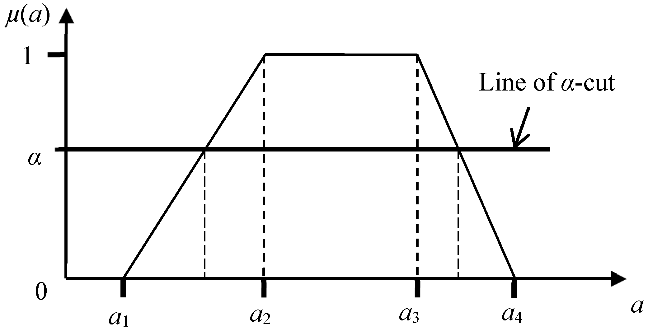
2.2. Fuzzy Numbers and Their Arithmetic

The degree-day method described above is conducted based on the “crisp values”. As some of these parametric values are subject to uncertainty, it is common to employ “representative values” (e.g., TMY) in the calculations to satisfy the requirement of using crisp values. In this context, the purpose of fuzzy numbers is to extend the degree-day method that allows the inputs and calculations of numerical intervals (instead of only representative crisp values).
This study adopts the trapezoidal fuzzy number (TrFN) as the general form to express numerical intervals. In the definition, suppose quantity ‘a’ represents a parameter in an equation (e.g., TA,t), and let Fa be the fuzzy number of quantity ‘a’. A TrFN can be expressed as a quadruple, i.e., Fa = (a1, a2, a3, a4), in which a1 represents the lower bound, a2 to a3 the range of typical values, and a4 the upper bound of quantity ‘a’. The membership function (denoted as µ(a)) of a TrFN is formulated below to reflect the likelihood of the actual value of quantity ‘a’.
μ ( a ) = { 0 a < a 1 a a 1 a 2 a 1 a 1 a < a 2 1 a 2 a < a 3 a a 4 a 3 a 4 a 3 a a 4 0 a > a 4
The advantage of TrFN is that it generalizes different types of numerical expressions. For example, a simple interval can be expressed via TrFN by setting a1 = a2 and a3 = a4. Similarly, TrFN can represent a triangular fuzzy number by setting a2 = a3, and a crisp number by setting a1 = a2 = a3 = a4. In other words, the generality of TrFN allows the inputs from pure crisp values to intervals and triangular numbers all under the TrFN definition.
To obtain a numerical interval from TrFN (denoted as [alow, aup]), the common α-cut operation is applied as presented in Figure 1 [33]. It helps to define the upper and lower bounds of the interval. For example, as presented in Figure 1, if α = 0.5, the interval will include the values with the membership above or equal to 0.5. Then, α-cut can be viewed as a horizontal line that intersects the fuzzy number and marks the upper and lower bounds. As observed, a higher α value will lead to a smaller interval.
The basic formulations of fuzzy number arithmetic are provided in Table 1 based on two fuzzy numbers Fa = (a1, a2, a3, a4) and Fb = (b1, b2, b3, b4), and a crisp number w. Notably, fuzzy number arithmetic has been studied in literature (e.g., [26,32]), and fuzzy number multiplication and division will not yield TrFN precisely. Thus, the common approximation (distinguished by the symbol “≈” in Table 1) is applied [33].

2.3. Application of Fuzzy Numbers to the Degree-Day Method

In this paper, two input parameters in the degree-day method are treated as fuzzy numbers: outdoor ambient temperature (denoted as FT_a,t) and furnace efficiency (denoted as Fη), which are formulated below.
FT_a,t = (Tt,1, Tt,2, Tt,3, Tt,4)
Fη = (η1, η2, η3, η4)
Regarding the outdoor ambient temperature, its fuzzy number can be interpreted as the range of the average values at the tth time period. For example, consider Day 1 as the time period, and its historical average outdoor ambient temperature in 10 years is −8 °C. At the same time, the average low of Day 1 is −15 °C, and the average high is 1 °C. In this case, the fuzzy number can be set as FT_a,t = (−15, −8, −8, 1) °C.
Regarding the furnace efficiency, its fuzzy number should be dependent on the HVAC equipment selection, and its value is based on the experience and judgment by engineers. Assuming a high-efficiency heating system is adopted, ηfr is about between 90% and 98.5% according to the Department of Energy, U.S. (http://energy.gov/energysaver/furnaces-and-boilers). By setting 90% and 98.5% as the lower and upper bounds, we roughly take the typical range as one third of the total range in the middle, and the corresponding fuzzy number is set as Fη = (0.90, 0.93, 0.96, 0.985).
After specifying the input uncertainty using fuzzy numbers, the next step is to apply these fuzzy numbers in the degree-day method. By approximating the integration in Equation (1) as a series of summations, the degree-day method can be executed using some basic arithmetic calculations (e.g., addition and multiplication). Then, fuzzy number arithmetic is applied in the degree-day method to propagate the input fuzzy numbers (i.e., FT_a,t and Fη) and determine the energy consumption (i.e., Ei) as an interval estimation. Let FΔT,t = (ΔTt,1, ΔTt,2, ΔTt,3, ΔTt,4) be the fuzzy number of the temperature difference between the balance point temperature (Tbal) and the fuzzy outdoor ambient temperature (i.e., Equation (7)) at the tth time period, and it can be formulated as follows.
Δ T t , j = { T b a l T t , j if   ( T b a l T t , j ) > 0   for   j   = 1 ,   2 ,   3 ,   4 0 otherwise
Let FDD_i and FE_i be the fuzzy numbers of the heating degree-days and energy consumption of the ith year, respectively. Their corresponding equations based on Equations (1) and (3) are formulated as follows.
F D D _ i = F Δ T , 1 F Δ T , 2 F Δ T , t F Δ T , T T i m e
F E _ i = ( K t o t F D D _ i ) F η
Let the fuzzy number of the energy consumption be FE_i = (Ei,1, Ei,2, Ei,3, Ei,4). Then, the interval of Ei (denoted as [Ei,low, Ei,up]) can be obtained by the α-cut operation, which is formulated as follows
[ E i , l o w ,   E i , u p ] = [ E i , 1 + α ( E i , 2 E i , 1 ) ,   E i , 4 α ( E i , 4 E i , 3 ) ]
If α = 0, the interval is equal to [Ei,1, Ei,4], representing the range of the results obtained by all possible combinations of input variations. For example, the upper bound (i.e., Ei,4, the highest possible energy consumption in a year) is obtained by having the historical daily average low (outdoor ambient) temperatures for all days in a year. In practice, this situation is very rare, and thus we suggest setting the values of α at least 0.3. Admittedly, a rigorous procedure to precisely set the values of α remains an open research question. In practice, as the values of α is inversely proportional to the sizes of intervals, the method practitioner can obtain the intervals at α = 0.3, 0.5 and 0.7 to reasonably examine the conservative (large), neutral, tight intervals, respectively.
Notably, the interval of Ei indicates the uncertainty in the energy consumption, and it is caused by the input uncertainty sources specified in Equations (7) and (8). Then, if the parameters of outdoor ambient temperatures and furnace efficiency are set as “crisp” values (e.g., using average points), the whole analysis is returned back to the traditional degree-day method. In other words, the proposed fuzzy degree-day method can be viewed as one extension of the degree-day method that can process the fuzzy variation type of uncertainty information. In the next section, a building example will be used to demonstrate and verify the fuzzy degree-day method.

3. Building Application and Verification

To demonstrate and verify the proposed fuzzy degree-day method, a building example from a Canadian city is used, along with the data of outdoor ambient temperatures in 52 years (from 1960 to 2011). Firstly, the standard degree-day method is applied to verify the adequacy of input parameters (e.g., Ktot). Then, the fuzzy degree-day method is applied, which results are compared to the variation of annual heating energy consumption in 52 years.

3.1. Application of the Degree-Day Method

The building example is a two-story property located in Calgary, Canada. The gross building area is 517.3 m2. The available space in the building is used as a rental property, where the first floor has the restaurant and the second floor is the office space. The restaurant located on the main floor is fully equipped with a commercial kitchen. The office space on the second floor has a lunch station equipped with a microwave and a refrigerator. The building does not have an elevator, and it can be accessed through the entrances at the front and back. For the design purpose, the following operating hours and indoor conditions are set for both the office and restaurant.
  • Operating hours
    • Restaurant: 11:00 a.m. to 1:00 a.m. (Tuesday to Sunday)
    • Office: 8:00 a.m. to 5:00 a.m. (Monday to Friday)
  • Indoor conditions (occupied)
    • Restaurant and office (summer): 21 °C (or 70 °F)
    • Restaurant and office (winter): 20 °C (or 68 °F)
  • Indoor conditions (unoccupied)
    • Restaurant and office (summer): 28 °C (or 82 °F)
    • Restaurant and office (winter): 18 °C (or 64 °F)
The weather information in Calgary was obtained from the website operated by the Government of Canada (www.climate.weather.gc.ca) [52]. To get some general impression, Table 2 provides the statistics of outdoor ambient temperature in Calgary from 1981 to 2010. As observed, Calgary generally experienced cold weather where the daily mean temperature ranges from −7.1 °C to 16.5 °C. Based on the available information from the government website, the temperature data from 1960 to 2011 are applied in this study.
The degree-day method discussed in the Section 2.1 is applied to the building example, and some key results are reported in Table 3. Regarding the outdoor ambient temperature, the hourly temperature data were used. To estimate the heat loss coefficient (Ktot) using Equation (5), the building envelope was analyzed to determine the U factor (i.e., ∑UAo) and the building’s volume (i.e., V), and the ventilation requirements were analyzed to determine the value of N. The balance point temperatures are estimated using Equation (4), where the internal temperature and the heat gain are based on the indoor conditions and usages. Since both floors are used for different purposes, the heat loss coefficient and balance point temperature are estimated separately for each floor. Notably, the heat loss of the first floor (i.e., −2246.1 W/°C) is considerably higher than that of the second floor (i.e., −717.8 W/°C) as the heat loss from the ground is higher than that from the roof. This also leads to the difference of the balance point temperatures between two floors.
The result of the degree-day method indicates the annual heating energy consumption is 236 × 103 kWh. To verify this value, we have also run the software simulation using eQuest® (version 3.65, http://www.doe2.com/equest/), and the corresponding result is 234 × 103 kWh. The percentage difference of these two values is less than 1%, and it is considered that the degree-day method yields a reasonable result in this case. Then, some parametric values (e.g., Ktot) will be used in the next sub-section for the fuzzy degree-day method.

3.2. Application of the Fuzzy Degree-Day Method and Verification

To apply the fuzzy numbers in the degree-day method, we first define the fuzzy numbers for the outdoor ambient temperature (i.e., FT_a,t). To specify this fuzzy number, we use the temperature variations in 52 years (from 1960 to 2011) based on the weather statistics discussed earlier. Also, the daily temperature data were used (instead of hourly temperatures) since the uncertainty of hourly temperatures can be too exhaustive, and it may potentially lead to the over interpretation of the results. By setting the time period as one day, Tt,1 is defined as the average of lowest outdoor ambient temperatures in 52 years on Day t, and Tt,4 is the average of highest temperatures on Day t. For example, T201,1 is the average of lowest outdoor ambient temperatures on July 21st (i.e., Day 201) in 52 years. Similarly, Tt,2 and Tt,3 are set equal to the daily average outdoor ambient temperature at the tth time period. Since Tt,2 = Tt,3 in the setting, the inputs of fuzzy outdoor ambient temperatures will be triangular fuzzy numbers. Regarding the furnace efficiency, its fuzzy number is set as Fη = (0.90, 0.93, 0.96, 0.985), as discussed in Section 2.3.
After specifying FT_a,t and Fη, Equations (10) and (11) are used to determine the fuzzy number of heating energy consumption, and the result is FE_i = (126, 216, 223, 365) (×103) kWh. Notably, the range of lower and upper bounds of this fuzzy number is quite large because both bounds are obtained by taking extreme values at each time period. For example, the lower bound 126 × 103 kWh is obtained by summing the lowest heating energy of each day in 52 years. This situation is very unlikely to happen in a single year.
Then, the α-cut operation is used to obtain the numerical interval. In this example, we set the α at three levels: 0.3, 0.5, and 0.7, to represent the conservative (large), neutral, tight intervals, respectively. The α-cut interval results are provided in Table 4. For example, by having α = 0.5, the typical energy consumption would vary between 171 and 294 (×103) kWh.
Since we have the historical data of outdoor ambient temperatures in 52 years, we can run the traditional degree-day method using this data and obtain the energy consumption for every single year. The variation of outdoor ambient temperature will then be reflected in the resulting values of yearly energy consumption. Table 5 shows the heating energy consumption in 52 years, where the lowest and highest values are 172 and 298 (×103) kWh, respectively. To verify further, we count the number of years which energy consumption is included in the α-cut intervals, and the results are provided in Table 4. As observed, the α-cut intervals can provide reasonable estimations for the range of energy consumption as they can cover the majority of historical energy consumption values.
In addition, Monte Carlo simulation is used to compare the results. In this simulation, we first convert the input fuzzy numbers (i.e., outdoor ambient temperature in Equation (7) and furnace efficiency in Equation (8)) into trapezoidal distributions (i.e., the area enclosed in the fuzzy number equal to one). Then, the outdoor ambient temperatures and the furnace efficiency are sampled from their distributions, and the energy consumption is determined based on the degree-day method. After running the simulation with 10,000 runs, we obtain the mean of the energy consumption equal to 224 kWh, with the minimum and maximum values as 214 kWh and 236 kWh, respectively. As observed, the results from Monte Carlo simulation exhibit a narrower range of variations, which includes 20 historical records (out of 52). Yet, they are all within the intervals in Table 4, and it verifies the proposed fuzzy method.
In sum, by using the traditional degree-day method, the energy consumption is estimated as 236 ×103 kWh, which is the average of energy consumption shown in Table 5. Beyond the average-point estimation, the fuzzy degree-day method can yield the interval of energy consumption. From the historical data verification, the variation of energy consumption due to the variation of outdoor ambient temperatures can be fairly reflected in the fuzzy degree-day method.

4. Closing Remarks

This paper presents a fuzzy degree-day method for estimating building heating energy consumption as numerical intervals. The proposed methodology processes the uncertainty of outdoor ambient temperatures and furnace efficiency as fuzzy numbers, which are used to extend the degree-day method for yielding numerical intervals in energy estimation. The fuzzy degree-day method has been applied to a building example, which results are comparable to the variation of heating energy consumption based on the data of outdoor ambient temperatures in 52 years.
In practice, the HVAC practitioners are required to identify the sources of uncertainty in the application of the degree-day method, and express them as intervals or fuzzy numbers. Then, they can apply the relevant techniques to obtain the numerical interval of energy consumption of an isolated building. Since parametric inputs may not be precisely confirmed at the early design stage, the degree-day method is an effective tool for prompt energy estimation. In this context, the fuzzy interval result can support certain risk-related decisions due to some extreme situations.
In the current methodological development, the proposed fuzzy degree-day method is limited to converting crisp values into fuzzy numbers, along with fuzzy number arithmetic for computation. One direction of future work is to incorporate other kinds of uncertainty such as indoor activities and work schedules (that influence the heat gains in the building) for propagating different uncertainties in the analysis of energy consumption. Also, it is desired to explore the theoretical framework that combines the statistical uncertainty (e.g., weather history) and the expert assessment (e.g., future building usages) based on probability and fuzzy set theories for the estimation of building energy consumption.

Acknowledgments

The first author received the financial support from the NSERC Discovery Grant.

Author Contributions

The authors have contributed equally in the preparation of this paper.

Conflicts of Interest

The authors declare no conflict of interest.

References

  1. Al-Homoud, M.S. Computer-aided building energy analysis techniques. Build. Environ. 2001, 36, 421–433. [Google Scholar] [CrossRef]
  2. Moreci, E.; Ciulla, G.; Lo Brano, V. Annual heating energy requirements of office buildings in a European climate. Sustain. Cities Soc. 2016, 20, 81–95. [Google Scholar] [CrossRef]
  3. Kohler, M.; Blond, N.; Clappier, A. A city scale degree-day method to assess building space heating energy demands in Strasbourg Eurometropolis (France). Appl. Energy 2016, 184, 40–54. [Google Scholar] [CrossRef]
  4. Sarak, H.; Satman, A. The degree-day method to estimate the residential heating natural gas consumption in Turkey: A case study. Energy 2003, 28, 929–939. [Google Scholar] [CrossRef]
  5. Valor, E.; Meneu, V.; Caselles, V. Daily air temperature and electricity load in Spain. J. Appl. Meteorol. 2001, 40, 1413–1421. [Google Scholar] [CrossRef]
  6. Moral-Carcedo, J.; Vicéns-Otero, J. Modelling the non-linear response of Spanish electricity demand to temperature variations. Energy Econ. 2005, 27, 477–494. [Google Scholar] [CrossRef]
  7. Azevedo, J.A.; Chapman, L.; Muller, C.L. Critique and suggested modifications of the degree days methodology to enable long-term electricity consumption assessments: A case study in Birmingham, UK: Critique and suggested modifications of the degree days methodology. Meteorol. Appl. 2015, 22, 789–796. [Google Scholar] [CrossRef]
  8. Amato, A.D.; Ruth, M.; Kirshen, P.; Horwitz, J. Regional energy demand responses to climate change: Methodology and application to the commonwealth of Massachusetts. Clim. Chang. 2005, 71, 175–201. [Google Scholar] [CrossRef]
  9. Guan, L. Preparation of future weather data to study the impact of climate change on buildings. Build. Environ. 2009, 44, 793–800. [Google Scholar] [CrossRef]
  10. Cox, R.A.; Drews, M.; Rode, C.; Nielsen, S.B. Simple future weather files for estimating heating and cooling demand. Build. Environ. 2015, 83, 104–114. [Google Scholar] [CrossRef] [Green Version]
  11. Coydon, F.; Herkel, S.; Kuber, T.; Pfafferott, J.; Himmelsbach, S. Energy performance of façade integrated decentralised ventilation systems. Energy Build. 2015, 107, 172–180. [Google Scholar] [CrossRef]
  12. Bolattürk, A. Determination of optimum insulation thickness for building walls with respect to various fuels and climate zones in Turkey. Appl. Therm. Eng. 2006, 26, 1301–1309. [Google Scholar] [CrossRef]
  13. Kurekci, N.A. Determination of optimum insulation thickness for building walls by using heating and cooling degree-day values of all Turkey’s provincial centers. Energy Build. 2016, 118, 197–213. [Google Scholar] [CrossRef]
  14. Verbai, Z.; Lakatos, Á.; Kalmár, F. Prediction of energy demand for heating of residential buildings using variable degree day. Energy 2014, 76, 780–787. [Google Scholar] [CrossRef]
  15. Mitchell, J.W.; Braun, J.E. Principles of Heating, Ventilation, and Air Conditioning in Buildings; Wiley: Hoboken, NJ, USA, 2013. [Google Scholar]
  16. American Society of Heating, Refrigerating and Air-Conditioning Engineers. 2013 ASHRAE Handbook, Fundamentals; American Society of Heating, Refrigerating and Air-Conditioning Engineers: Atlanta, GA, USA, 2013. [Google Scholar]
  17. Zimmermann, H.J. Fuzzy Set Theory and Its Applications; Kluwer Academic Publishers: Norwell, MA, USA, 2001. [Google Scholar]
  18. Guyonnet, D.; Bourgine, B.; Dubois, D.; Fargier, H.; Come, B.; Chilès, J.-P. Hybrid approach for addressing uncertainty in risk assessments. J. Environ. Eng. 2003, 129, 68–78. [Google Scholar] [CrossRef]
  19. Baudrit, C.; Dubois, D.; Guyonnet, D. Joint propagation and exploitation of probabilistic and possibilistic information in risk assessment. IEEE Trans. Fuzzy Syst. 2006, 14, 593–608. [Google Scholar] [CrossRef]
  20. Thom, H. Seasonal degree-day statistics for the United States. Mon. Weather Rev. 1952, 80, 143–147. [Google Scholar] [CrossRef]
  21. Lam, J.C.; Hui, S.C.M.; Chan, A.L.S. A statistical approach to the development of a typical meteorological year for Hong Kong. Archit. Sci. Rev. 1996, 39, 201–209. [Google Scholar] [CrossRef]
  22. Janjai, S.; Deeyai, P. Comparison of methods for generating typical meteorological year using meteorological data from a tropical environment. Appl. Energy 2009, 86, 528–537. [Google Scholar] [CrossRef]
  23. Pusat, S.; Ekmekçi, İ.; Akkoyunlu, M.T. Generation of typical meteorological year for different climates of Turkey. Renew. Energy 2015, 75, 144–151. [Google Scholar] [CrossRef]
  24. Kneifel, J.D.; O’Rear, E.G. An Assessment of Typical Weather Year Data Impacts vs. Multi-Year Weather Data on Net-Zero Energy Building Simulations; Report No. NIST SP 1204; National Institute of Standards and Technology: Gaithersburg, MD, USA, 2016.
  25. Dubois, D.; Prade, H. Fuzzy sets and probability: Misunderstandings, bridges and gaps. In Proceedings of the Second IEEE International Conference on Fuzzy Systems, San Francisco, CA, USA, 28 March–1 April 1993; pp. 1059–1068. [Google Scholar]
  26. Giachetti, R.E.; Young, R.E. A parametric representation of fuzzy numbers and their arithmetic operators. Fuzzy Sets Syst. 1997, 91, 185–202. [Google Scholar] [CrossRef]
  27. Schjær-Jacobsen, H. Comparison of probabilistic and possibilistic approaches to modelling of economic uncertainty. In Proceedings of the 8th Workshop on Uncertainty Processing 2009, Liblice, Czech Republic, 19–23 September 2009; pp. 213–225. [Google Scholar]
  28. Michalik, G.; Khan, M.E.; Bonwick, W.J.; Mielczarski, W. Structural modelling of energy demand in the residential sector: 2. The use of linguistic variables to include uncertainty of customers’ behaviour. Energy 1997, 22, 949–958. [Google Scholar] [CrossRef]
  29. Ciabattoni, L.; Grisostomi, M.; Ippoliti, G.; Longhi, S. Fuzzy logic home energy consumption modeling for residential photovoltaic plant sizing in the new Italian scenario. Energy 2014, 74, 359–367. [Google Scholar] [CrossRef]
  30. Kolokotsa, D. Artificial intelligence in buildings: A review of the application of fuzzy logic. Adv. Build. Energy Res. 2007, 1, 29–54. [Google Scholar] [CrossRef]
  31. Zadeh, L.A. Fuzzy logic and approximate reasoning. Synthese 1975, 30, 407–428. [Google Scholar] [CrossRef]
  32. Dubois, D.; Prade, H. Operations on fuzzy numbers. Int. J. Syst. Sci. 1978, 9, 613–626. [Google Scholar] [CrossRef]
  33. Lee, K.H. First Course on Fuzzy Theory and Applications; Springer: Berlin, Germany, 2006. [Google Scholar]
  34. Singer, D. A fuzzy set approach to fault tree and reliability analysis. Fuzzy Sets Syst. 1990, 34, 145–155. [Google Scholar] [CrossRef]
  35. Cheng, C.H.; Mon, D.L. Fuzzy system reliability analysis by interval of confidence. Fuzzy Sets Syst. 1993, 56, 29–35. [Google Scholar] [CrossRef]
  36. Moens, D.; Hanss, M. Non-probabilistic finite element analysis for parametric uncertainty treatment in applied mechanics: Recent advances. Finite Elem. Anal. Des. 2011, 47, 4–16. [Google Scholar] [CrossRef]
  37. Erdogan, Y.S.; Bakir, P.G. Inverse propagation of uncertainties in finite element model updating through use of fuzzy arithmetic. Eng. Appl. Artif. Intell. 2013, 26, 357–367. [Google Scholar]
  38. Wang, C.; Qiu, Z.; Xu, M. Collocation methods for fuzzy uncertainty propagation in heat conduction problem. Int. J. Heat Mass Transfer. 2017, 107, 631–639. [Google Scholar] [CrossRef]
  39. Maskey, S.; Guinot, V.; Price, R.K. Treatment of precipitation uncertainty in rainfall-runoff modelling: A fuzzy set approach. Adv. Water Resour. 2004, 27, 889–898. [Google Scholar] [CrossRef]
  40. Scherm, H. Simulating uncertainty in climate–pest models with fuzzy numbers. Environ. Pollut. 2000, 108, 373–379. [Google Scholar] [CrossRef]
  41. Wu, D.; Gao, W.; Wang, C.; Tangaramvong, S.; Tin-Loi, F. Robust fuzzy structural safety assessment using mathematical programming approach. Fuzzy Sets Syst. 2016, 293, 30–49. [Google Scholar] [CrossRef]
  42. Dubois, D. An application of fuzzy arithmetic to the optimization of industrial machining processes. Math. Modell. 1987, 9, 461–475. [Google Scholar] [CrossRef]
  43. Wang, L.; Mathew, P.; Pang, X. Uncertainties in energy consumption introduced by building operations and weather for a medium-size office building. Energy Build. 2012, 53, 152–158. [Google Scholar] [CrossRef]
  44. Day, A.R.; Knight, I.; Dunn, G.; Gaddas, R. Improved methods for evaluating base temperature for use in building energy performance lines. Build. Serv. Eng. Res. Technol. 2003, 24, 221–228. [Google Scholar] [CrossRef]
  45. Layberry, R.L. Degree days for building energy management—Presentation of a new data set. Build. Serv. Eng. Res. Technol. 2008, 29, 273–282. [Google Scholar] [CrossRef]
  46. Layberry, R.L. Analysis of errors in degree days for building energy analysis using Meteorological Office weather station data. Build. Serv. Eng. Res. Technol. 2009, 30, 79–86. [Google Scholar] [CrossRef]
  47. Day, A.R. An improved use of cooling degree-days for analysing chiller energy consumption in buildings. Build. Serv. Eng. Res. Technol. 2005, 26, 115–127. [Google Scholar] [CrossRef]
  48. De Rosa, M.; Bianco, V.; Scarpa, F.; Tagliafico, L.A. Heating and cooling building energy demand evaluation; a simplified model and a modified degree days approach. Appl. Energy 2014, 128, 217–229. [Google Scholar] [CrossRef]
  49. Shin, M.; Do, S.L. Prediction of cooling energy use in buildings using an enthalpy-based cooling degree days method in a hot and humid climate. Energy Build. 2016, 110, 57–70. [Google Scholar] [CrossRef]
  50. Day, A.R.; Karayiannis, T.G. Identification of the uncertainties in degree-day-based energy estimates. Build. Serv. Eng. Res. Technol. 1999, 20, 165–172. [Google Scholar] [CrossRef]
  51. Ning, M.; Zaheeruddin, M. Fuzzy set-based uncertainty analysis of HVAC&R systems: A simulation study. Build. Serv. Eng. Res. Technol. 2009, 30, 241–262. [Google Scholar]
  52. Government of Canada. Historical Climate Data. Available online: www.climate.weather.gc.ca (accessed on 15 April 2015).
Figure 1. Illustration of a trapezoidal fuzzy number and α-cut interval (where μ(a) is the membership function, and α is the minimum membership value that defines the upper and lower bounds of the interval).
Buildings 08 00021 g001
Table 1. Fuzzy arithmetic based on trapezoidal fuzzy number (TrFN).
Fuzzy number addition F a w = ( a 1 + w , a 2 + w , a 3 + w , a 4 + w ) F a F b = ( a 1 + b 1 ,   a 2 + b 2 ,   a 3 + b 3 ,   a 4 + b 4 )
Fuzzy number subtraction F a w = ( a 1 w , a 2 w ,   a 3 w ,   a 4 w ) F a F b = ( a 1 b 1 ,   a 2 b 2 ,   a 3 b 3 ,   a 4 b 4 )
Fuzzy number multiplication F a w = ( a 1 × w ,   a 2 × w ,   a 3 × w ,   a 4 × w ) F a F b ( a 1 × b 1 ,   a 2 × b 2 ,   a 3 × b 3 ,   a 4 × b 4 )
Fuzzy number division F a w = ( a 1 / w ,   a 2 / w ,   a 3 / w ,   a 4 / w ) F a F b ( a 1 / b 4 ,   a 2 / b 3 ,   a 3 / b 2 ,   a 4 / b 1 )
Table 2. Monthly data of outdoor ambient temperatures in Calgary from 1981 to 2010 [52].
MonthRecord Low Average LowDaily MeanAverage HighRecord High
Jan.−44.4 °C−13.2 °C−7.1 °C−0.9 °C17.6 °C
Feb.−45.0 °C−11.4 °C−5.4 °C0.7 °C22.6 °C
Mar.−37.2 °C−7.5 °C−1.6 °C4.4 °C25.4 °C
Apr.−30.0 °C−2.0 °C4.6 °C11.2 °C29.4 °C
May−16.7 °C3.1 °C9.7 °C16.3 °C32.4 °C
Jun.−3.3 °C7.5 °C13.7 °C19.8 °C35.0 °C
Jul.−0.6 °C9.8 °C16.5 °C23.2 °C36.1 °C
Aug.−3.2 °C8.8 °C15.8 °C22.8 °C35.6 °C
Sep.−13.3 °C4.1 °C11.0 °C17.8 °C33.3 °C
Oct.−25.7 °C−1.4 °C5.2 °C11.7 °C29.4 °C
Nov.−35 °C−8.2 °C−2.4 °C3.4 °C22.8 °C
Dec.−42.8 °C−12.8 °C−6.8 °C−0.8 °C19.5 °C
Table 3. Results of the degree-day method.
The U Factor (∑UAo)1400.8 W/°C
The ventilation factor (NV)4689.5 W/°C
Total heat loss coefficient (Ktot)2963.9 W/°C
Heat loss coefficient of the 1st floor (Ktot_1)2246.1 W/°C
Heat loss coefficient of the 2nd floor (Ktot_2)717.8 W/°C
Average balance point temperature of 1st floor (Tbal_1)13.4 °C
Average balance point temperature of 2nd floor (Tbal_2)1.5 °C
Furnace efficiency (ηfr)0.95
Energy consumption estimated by the degree-day method236 × 103 kWh
Energy consumption estimated by eQuest®234 × 103 kWh
Table 4. Interval results and verification with different α-cut operations.
α Levelα-Cut Interval% Number of Years Included in the α-Cut Interval
α = 0.3[Ei,low, Ei,up] = [153, 322] (×103) kWh100%
α = 0.5[Ei,low, Ei,up] = [171, 294] (×103) kWh98% (1 year excluded)
α = 0.7[Ei,low, Ei,up] = [189, 266] (×103) kWh85% (8 years excluded)
Table 5. Heating energy consumption in 52 years using the degree-day method.
YearEnergy Consumption (103 kWh)YearEnergy Consumption (103 kWh)YearEnergy Consumption (103 kWh)YearEnergy Consumption (103 kWh)
1960242197324519862021999204
1961234197423019871722000245
1962228197525919882022001218
1963226197620319892352002246
1964250197722819902272003239
1965274197826519912132004215
1966271197925519922112005210
1967259198024019932222006212
1968253198118819942342007219
1969275198227419952502008229
1970265198323119962982009245
1971261198423219972312010224
1972278198523819982332011232

