Debt and Deficit Growth Rate Reporting for Post-Communist European Union Member States


1
Department of Economic Policy, Faculty of Economics, University of Gdansk, 80309 Gdansk, Poland
2
Polo Centre of Sustainability, 18100 Imperia, Italy
3
Faculty of Economics, University of Gdansk, 80309 Gdansk, Poland
*
Authors to whom correspondence should be addressed.
Soc. Sci. 2019, 8(6), 173; https://doi.org/10.3390/socsci8060173
Submission received: 30 April 2019
/
Revised: 3 June 2019
/
Accepted: 4 June 2019
/
Published: 5 June 2019
(This article belongs to the Special Issue Measuring Efficiency Considering Efficacy, Fairness and Uncertainty: Current Trends in Methods, Practice and Policies)
Abstract
:A focalized analysis and reporting on the problems of general government debt (GGD) and government deficit (GD) and their influencing factors on economic growth rate tell the story of positive, neutral, and negative economies. Research was conducted over a nineteen-year period between 2000 and 2018 on all eleven post-communist European Union Member States (MS). MSs are divided in to three regional blocks: (1) the Baltic countries, (2) Central and Eastern European countries, and (3) the Balkan countries. Reviewed literature examined different types of GGD and GD with denoted influence on each MS’s economy and government. GGD and GD increase as a result of State intervention by reacting to economic fluctuations needed in creating redistributive-related fiscal policy. A breakdown of the problems of fiscal policy is explained. Datasets were compiled and systematically analyzed using Eurostat indicators. European regulatory benchmarking was used for GGD and GD as a percentage of gross domestic product. Results were divided at the regional group level. Comparative tax systems based on total general government revenue as well as total tax and contribution rate were evaluated. Histo-geographical research was considered and a comparative examination of GGD, GD and growth rate illustrated. In terms of GGD, GD, and growth rate, the Baltic countries were best situated, while all other countries were generally stable—with the exception of Hungary, Croatia, and Slovenia. In all, negative or stagnant periods revealed a general positive trend throughout the study with the exception of the world financial crisis of 2008, in which a deteriorative impact on growth rate was evident in all MS—especially from 2009. In the latter years, MSs’ economic promise signals a high potential for renewed public finance and stability initiatives.
1. Introduction
General government debt (GGD) is defined as all liabilities deriving predominately from credits of public institutions (i.e., a government’s central budget, public territorial entities, funds, and agencies). A lengthened definition would include the sum of previous years’ government deficit (GD) as well as liabilities from the State from credits to cover such GD (Marciniak 2013; Yang et al. 2018; Hyman 2018). In most cases, GGD occurs when State indebtedness from domestic and foreign creditors is issued through treasury bills, notes and bonds as well as bank credit. GGD and GD are interlaced with public finance and fundamentally influence economic growth, particularly via investment. Concerns of high GGD and GD can rebound and negatively affect a country’s economic success. A principal reason for the augmentation of GGD is the necessity of credit to cover GD. This sometimes creates a cyclic process if only GD is addressed and GGD is not. As a result, public credit is used to pay off GD from returnable inflows from a central budget, while financing credit for GGD generates costs of public finance (Kosek-Wojnar et al. 1994; OECD 2013). These costs are usually stretched over time, often having a generational effect and forcing future governments to deal with an unremitting GGD. In an examination of fiscal policy in post-communist European Union (EU) Member States (MS), the connection with GGD and GD and the core question of how they destabilize economic growth is reported on (Van Der Veer and Haverland 2018). Additional inquiries look at tools that best alleviate GGD and GD and relating negative influences from political determinants (e.g., policy), historical relations, and cultural norms.
A simple yet unsound method of overcoming GGD is inflation generated, by the printing of money, by central banks—an action generally forbidden in most developed countries. When a central bank (i.e., monetary authority) decides on this type of policy, it is usually based on short-term interest to immediately decrease purchasing power parity within the dominant part of society and limit entrepreneurial activity. Central banks operate independently from State government and are responsible for monetary policy, which has a direct effect on the inflation rate (Pegkas 2018). During periods of inflation, a negative outcome will affect everyone except the State, which experiences a taxflation effect (i.e., when inflation decreases GGD and GD from higher inflows of taxation). These inflows do not change public finance indexation since core adjustments to the taxation threshold are based on consumer price index limits. Moreover, since annual budgetary expenditure does not change, based on budget threshold, public finance will remain a key beneficiary of any implemented inflation-based tax (i.e., core to annual budgetary expenditure). The OECD (OECD 2017) considers several types of GGD as essential to an economy’s health and key to the sustainability of government finance, they include: (1) domestic vs. foreign—both dependent on currency value and ownership of debt (i.e., citizenry or institutions); (2) short-term (i.e., liquidity for an established budget) against long-term expenditure (e.g., property); (3) gross (i.e., the ability to cover public liabilities either of domestic or foreign entities that are not part of the public sector) versus net (i.e., gross GGD minus the liabilities from nonpublic entities within the public sector); (4) nominal value of liabilities versus real value (i.e., nominal values revised by inflation); (5) real (i.e., required liabilities of balance) versus potential (i.e., guarantees provided by the public sector); (6) central (i.e., the central State) versus local (i.e., self-government); and (7) declared versus hidden (i.e., other financial contracts and State liabilities for future expenditures (e.g., retired persons and annuitants)) (Dzwonkowski 2013; Tobera 2013; Łaszek 2013; Altiparmakov 2018; Högenauer and Howarth 2019). These types of GGD allow us to consider the specific origin of debt by making it easier to understand, observe, and reduce it. To better piece together this problem, we analyzed GGD utilizing two strategic perspectives of debt: valuably recognized and comparative. Valuably recognized debt is the sum of money, of a given currency, which government has indebted for creditors. Comparative debt elucidates the percentage ratio of GGD to gross domestic product (GDP) and applies it to GGD in an annual percentage format of GDP. In this paper, we observed historical fiscal data in all eleven post-communist EU MSs utilizing these observational perspectives. GGD and GD increase as a result of State intervention, which can react to economic fluctuations needed in creating redistributive-related policy (Wiśniewski 2015; Ćwikliński 2004; Neck and Sturm 2008). A breakdown of the paper is structured as follows: Section 2 explores problems in fiscal policy, Section 3 contains the methodology, Section 4 illustrates the results, Section 5 elucidates a discussion on tax system evaluation and conditions of public finance, and Section 6 the conclusion.
2. Problems of Fiscal Policy
2.1. Government Deficit
Government budget is used to define the methods of calculating income and outcome. GD, a negative balance in the government budget, occurs when such a budget exceeds its income in a given year. To account for the negative balance, capital inflow is usually eliminated in public sector entities (Neumann and Paczoski 2014). As such, different methodologies have been employed to assess how countries balance their budget, with notable primary bodies including the International Monetary Fund (IMF) and the EU. The IMF’s methodology uses government finance statistics by categorizing government-run public sectors via the central budget, State and local budgets, social security funds (e.g., resort enterprises), and noncommercial institutions that control and finance the State. Within an IMF framing, expenditures are monetary sources relevant to equivalent and non-equivalent, current and capital, and grants and loans. All of these means are consolidated by excluding transactions between public entities (Wernik 2001; Kim et al. 2018).
Within the EU, public finance is based on the European System of National and Regional Accounts. This accounting system measures assets and liabilities that adjust throughout the public sector (Wernik 2001). Difference in assets include cash, deposits, other securities, given loans, stocks and capital shares, mercantile credit, and advance payments. The balancing of one’s budget was standard until the 19th Century when the economic crisis of 1929 hit the world. In Keynesian theory, GD was seen as a solution for such an economic situation. Instituted, it meant the implementation of a systematic budget in which GD was an acceptable manner of activating an economy, forcing expenditures to become cumbersome fiscal structures; nonetheless, this idea was backed with the concept that it would stimulate global demand. Supporters were attentive in postponing GD and its payback without taking loss. This activity, to the detriment of much of the world, brought inflation and increased interest rates to financial markets (Gradoń 2003; Ari et al. 2018; Ortiz-Rodríguez et al. 2018).
Another form of budgetary management is a cyclical budget. In such a budget, it is expected that GD during a recession will neutralize budget surplus and stall economic growth. Henceforward, the State is forced to support the economy by augmenting public expenditure and, thus, its GD. One concern with the use of a cyclical budget approach are political targets or government motivation to persuade its electorate of social expenditure requisites and shortcomings (Gaudemet and Molinier 2000). However, based on impasse theory, it is possible to evaluate a cyclical budget’s GD in terms of threshold and given conditions. Impasse is defined as all impositions above income, foreseen within an annual budget, dependent on the status quo for the future economy. As a result, GD may occur as a result of the following two conditions, when: (1) Supplementary money is issued without increasing volume of production to avoid inflation and depreciation of the currency; and (2) utilizing a higher inflation mechanism to increase savings, and supply of goods and services (i.e., by applying a quantity impasse approach) (Gradoń 2003). To that end, GD can also be structural and correlate with the full rate of employment. In terms of these practices, cyclical fluctuations can be averted, which can influence budget and automatic economic stabilizers for better—active and passive—fiscal policy (Gradoń 2003). Using these methods, GD can be used to correct for inflation and instability.
2.2. General Government Debt and the Effect of Instability in Public Finance
In Keynesian theory, a school of thought based on the welfare state, active economic policy—particularly fiscal policy—has had negative, far-reaching effects on GGD and GD. Nonetheless, governments that spend money on investments utilizing GGD have found added value, irrespective of consequence. These investments have been found to bring financial return through taxation of private companies that are users of public investment. For example, government investment on transport infrastructure will develop private sector entities that cater to a transport niche. As such, according to Keynesian theory, GGD and GD will decrease savings while still stimulating an aggregated supply. Higher GD (i.e., in this case, from a decrease in savings) will result in the raising of interest rates to stimulate the crowding effect on private investment (Ball and Mankiw 1995). The stability of prices will bring increased production and better economic success. Even though GD can be considered a beneficial tool for the economy, during a recession, some argue for the use of automatic stabilizers as better mechanisms in neutralizing economic fluctuations (Ćwikliński 2004)—as such a number of outlooks should be considered.
In Ricardian theory, the GD is neutral; it has no influence on national savings or aggregated supply due to a decreasing emphasis on public savings. It utilizes the comparative advantage principle by pressing consumers to offset GD with the notion that higher taxes will be implemented in the future, allowing them to spend more of their income in the present. As such, any changes in taxes and public expenditure have no influence on aggregated demand (Barro 1988). In contrast with each other, Keynesian theory and Ricardian theory both attempt to better fiscal policy and reduce GD by creating economic improvement and stability. A notable example contrasting the two theories can be found in Giavazzi and Pagano’s (Giavazzi and Pagano 1990) research comparing Denmark and Ireland throughout the 1980s.
As such effects of restrictive fiscal policy are not linear (i.e., non-Keynesian), the same policy in different conditions can bring unexpected and, often, atypical results. When public finance is in good order (i.e., GGD and GD are under control and not abnormally high), solutions from fiscal policy can often resemble Keynesian-like aftereffects. Restrictive fiscal policy can sometimes improve an economic situation by accelerating a variety of economic conditions (Brzozowski et al. 2006; Alesina and Ardagna 1998; Hemming et al. 2002; Compant et al. 2005; Ardagna 2004). A useful example includes permanent income in which reaction to demand reflects the attitude of the consumer. In retrospect, it is particularly important to take into account how consumers react to fiscal policy (i.e., changes to taxes and public expenditures). A high GGD and GD can often create a dire situation for public finance in which consumers expect higher taxes which, retrospectively, will decrease income. In this way, demand is lessened and the potential for recession high. Conversely, when governments avoid high levels of GGD and GD, permanent income and demand go up, complementing consumers’ expectation that no changes in taxes or expenditure will be problematic. In this case, fiscal policy mitigation is advantageous yet limited in terms of its long-term effectiveness.
As a result, when we take into consideration why economic crises commence, there are a number of correlating reasons that are connected to high levels of GGD. Effects of crises exert pressure on government to decrease GD by lowering wages in the public sector and cutting social transfers. Another relating issue incorporates high interest rates via the banking sector, which causes withdrawal of foreign capital and, ultimately, leads to a decrease in investment and financial trouble for enterprises—increasing the probability of bankruptcy and default. This dangerous precedent shocks the banking sector, which is often a contributing factor to most financial crises. High inflation can be an aftereffect, with consequential factors including the decrease in production, increase in unemployment, and a worsen standard of living (Romer et al. 2000).
Changes to the amount and structure of income, as well as expenditure, can affect economic progress. A country’s level of savings can also influence economic growth (i.e., via the endogenous growth model) in terms of pace and return rate from private capital (Brzozowski et al. 2006). Expenditures, which are productive in developing infrastructure, can stimulate economic development society-wide (Kneller et al. 1999; Barro and Sala-i-Martin 2004). As such, crowding effects may arise if repayment of GGD leads to a decrease in public and private investment (Minea and Villieu 2010). Economic growth can be lowered and even halted if household consumption and domestic savings drastically fall (Saint-Paul 1992). High foreign debt can also service GGD by influencing the economy and investors alike (Neck and Sturm 2008). Foreign creditors can engender business thinking as well as GDP repayment of foreign debt (Krugman 1988; Alaimo et al. 2008). Similarly, this works for countries that do not have a problem with GGD by establishing high foreign investment correlating high external, international influence.
Conversely, instability in economic policy (i.e., on a macroeconomic level) directly relates to the risk of losing on investment (Eaton 1993; Serven 1997; Agénor and Montiel 2005). As such, most studies indicate the influence of GGD on economic growth (i.e., related to investments) as negative (Deshpande 1997; Pattollo et al. 2011; Clements et al. 2003; Shah et al. 2017; Smyth and Hsing 1995; Lin and Sosin 2001; Brzozowski et al. 2006). Cross-sectional analysis comparing developed and developing countries indicates GGD as a negative factor on economic growth (N’Zue 2018; Brzozowski et al. 2006; Pegkas 2018). Positive indicators include political stability, rule of law, and a high-quality, functional public sector. Inversely, negative indicators encompass a high rate of inflation, increasing taxes and disadvantageous changes to the law. These problems can severely influence private entrepreneurial activities and overall profit. Hence, if the quality of public institutions in a given country is high, there is most likely limited to no problem with GGD and the negative influence of GGD on the economy.
One important comparison in examining the influence of GGD on the economy is to consider positive and negative side-effects. The following are problematic GGD concerns relating to this dilemma. They include: (1) the possibility of raising taxes for higher inflows for the budget (i.e., the need for repayment of public debt) and repossession of private savings; (2) a poor international reputation which may have high value for public debt; (3) the cost of financial attendance; (4) the risk related to the exchange rate if GGD is issued in a foreign currency; (5) financial instability and bankruptcy; (6) the crowding out effect; (7) the deterioration and balancing of current accounts to balance out payments; (8) unstable rules for entrepreneurs; and (9) the decrease of a dynamism to the economy (Neumann and Paczoski 2014). As such, instability in public finance is a problem at the international level. Specifically, to test this problem, the paper applied the Maastricht Treaty and the Stability and Growth Pact (SGP) as two legislative benchmarks for best practices reporting. The Maastricht Treaty defines GD as net borrowing (i.e., increased indebtedness minus increased liabilities). These legislative regulations implemented at the European level, specifically within post-communist EU MSs, can foster economic destabilization, oblige the private sector and citizenry to pay higher taxes due to repayment requisites, and have a prolonged effect on future generations. At length, the paper reports and focalizes, in relation to the problems of fiscal policy, on integrating stabilization recommendations within the concerned MSs’ economic systems and highlights best practices to decrease GGD and GD.
3. Methodology
A systematic literature review was conducted using the following electronic journal databases: Science Direct, Web of Knowledge, Scopus, Science Direct, ProQuest, Sage, Directory of Open Access Journals, Google Scholar, and Google. In particular, we utilized a three-stepladder search by adding keywords to each step (i.e., sx), where “x” = each keyword in step 1. The following English language keywords frame step 1: “general government debt”, “government deficit”, “economic policy”, “economic growth rate”, “post-communist economy”, “economic consequences”, “economic trends”, “regional variation”, “political stability”, “government avoidance”, “economic change”, “GDP”, “European economic treaties”, “stability + regulations”, “Maastricht Treaty”, “Stability and Growth Pact”, “debt tools”, and “economic development”. Next, step two repeated the process with each of the following EU MS: “sx + Estonia”, “sx + Latvia”, “sx + Lithuania”, “sx + Czech Republic”, “sx + Hungary”, “sx + Poland”, “sx + Slovakia”, “sx + Bulgaria”, “sx + Croatia”, “sx + Romania”, and “sx + Slovenia”. Finally, step three repeated the process by searching for grouped blocks (i.e., regions) plus adding the word “countries” as well as jointly-searching countries from each block: “sx + Baltic + countries”, “sx + Estonia + Latvia + Lithuania”, “sx + Central European + Eastern European + countries”, “sx + Czech Republic + Hungary + Poland + Slovakia”, “sx + Balkan + countries”, and “sx + Bulgaria + Croatia + Romania + Slovenia”.
The literature was compiled, and the publications were systematically analyzed so as to identify those that presented specific findings relating to regulation-reporting of GGD and GD of 60% and 3% of GDP, respectively. These benchmark figures are taken from the Maastricht Treaty and the SGP (European Council 1997; Neck and Sturm 2008). We examined post-communist EU MSs’ GGD and GD using strategic and critical reading methods (Matarese 2013; Renear and Palmer 2009). As part of the systematic review process, we also identified past and existing terminology related to GGD and GD and synthesized and updated it so as to provide a way forward with the benchmark research.
The study examined all eleven post-communist EU MSs. We clustered these countries into three regional blocks and compared them by analyzing Eurostat indicators via its database, as follows: (1) the Baltic countries: Estonia, Latvia, and Lithuania; (2) Central and Eastern European countries: Czech Republic, Hungary, Poland, and Slovakia; and (3) the Balkan countries: Bulgaria, Croatia, Romania, and Slovenia (Figure 1).
From the regional blocks, we used macroeconomic data to create datasets within a nineteen-year period between 2000 and 2018. We then compared GGD and GD with economic growth, according to high and low indicators, among countries within each regional block. We charted each country to define national and regional trends, dynamic variability, and fiscal policy conditions of GGD and GD. Then, fiscal policy was examined by observing influence-related trends on growth rate and an overall analysis between regional groups—defined via country-specific economic policy. Finally, Section 5 addresses the tax systems in each MS by comparing datasets from Eurostat and the World Bank.
4. Results
Each of the three regional blocks (i.e., (1) the Baltic countries, (2) Central and Eastern European countries, and (3) the Balkan countries) is presented as a separate subsection. Regional blocks are illustrated in two parts: tabular data and two graphical charts.
4.1. The Baltic Countries
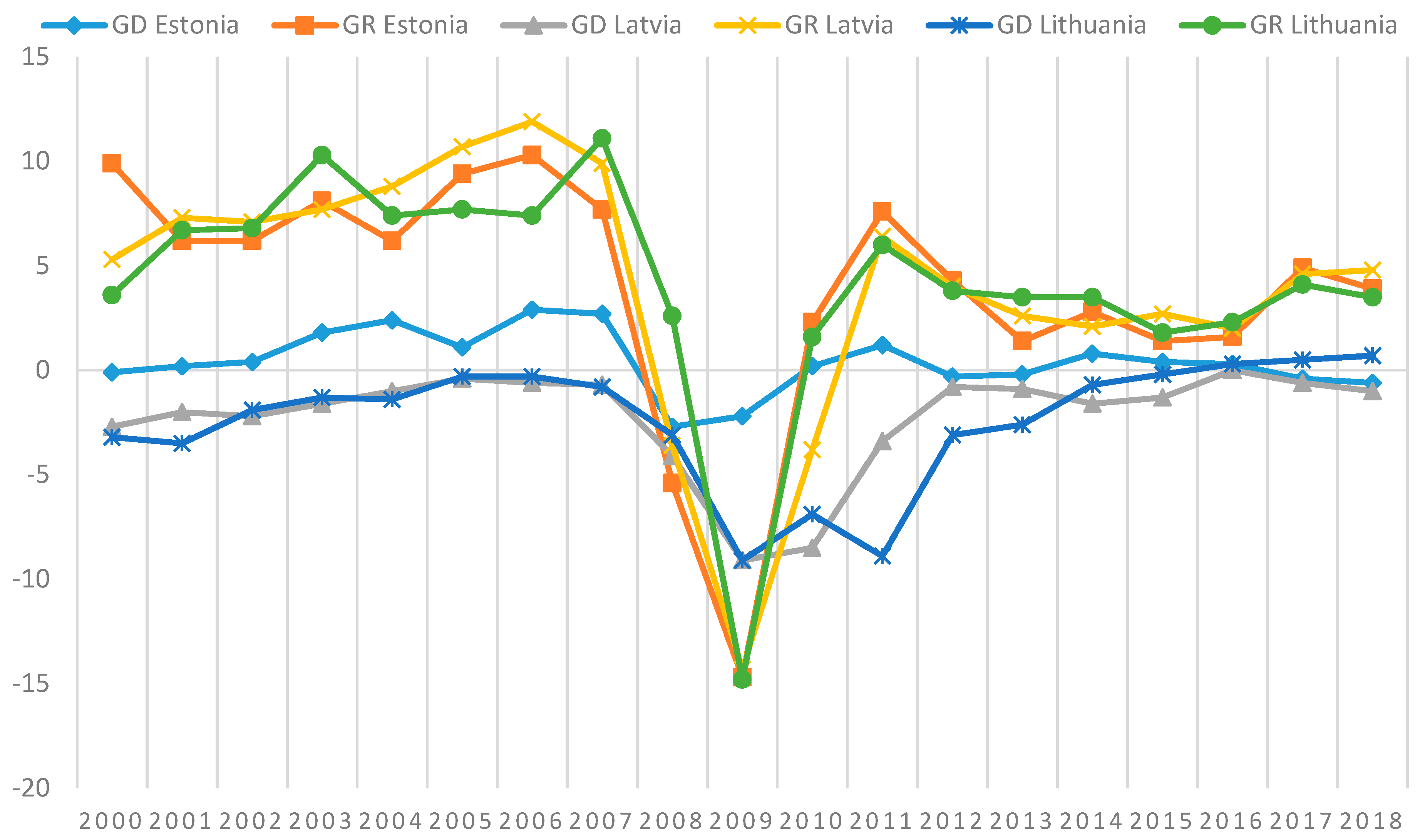
The Baltic countries had stable and normalized GGD and GD for most of the nineteen-year study (Table 1). In terms of the lowest level of GGD, Estonia was in the top position—worldwide, in fact. Its government surplus throughout all of the study remained in single digits, with the exception of 2014 when GGD reached 10.4%. Between 2000 and 2007, the country recorded exceptionally low levels of GGD before a slight augmentation during the then world financial crisis and recession period of 2009–2010 (Figure 2). As a consequence, Estonia’s growth rate remained low during the period of 2013–2018, with the GD floating around 9% of GDP—slightly higher from the previous decade, 2000–2010 (Figure 3). It should be noted that the country is in good standing in terms of GD and obtained a government surplus via its GD in 2000, 2008–2009, 2012–2013, and 2017–2018.
For the study period, both Latvia and Lithuania’s GGD remained below the recommended level of 60% (Table 1). Latvia safely controlled its GD until the financial crisis of 2008–2011, by managing to retain the recommended level after 2011 (Figure 2). On other hand, Lithuania’s GD remained higher than 3% of GDP in 2000–2001 and was up to 3% GDP between 2008 and 2012. Lithuania recorded the recommended level before the financial crisis (Figure 3). Latvia’s growth rate was high from 2000–2007 then during the recorded recession between 2008 and 2010. After 2010, the Latvian economy started to grow. Despite a slowing down from 2009, both Latvia and Lithuania recorded high growth rates up to 2007. Interestingly, Lithuania’s growth had a different accelerated rate from 1.6% to 4.1% GDP in 2010–2017. In summary on a regional scale, the Baltic countries achieved the best public financial outputs among the three regional blocks. Their economic growth was high while registering low levels of GGD and GD.
4.2. Central and Eastern European Countries
In Central and Eastern European countries, a relatively safe level of GGD was recorded—with the exception of Hungary in 2005, which had more than the recommended 60% of its GDP in 2005 (Table 2). The Czech Republic recorded a low GGD (i.e., below 30% of GDP) in 2000–2008 while maintaining a moderately high growth rate between 2003 and 2007. The world financial crisis decreased the country’s growth rate to 4.8% in 2009, which most probably forced the GGD to rise to more than 40% of its GDP in the following years. There was some fluctuation after 2009, but it stabilized after 2014, when the GGD of GDP finally decreased below 40% (Figure 4). Recently, in the last three years, a downward trend in GGD emerged from 37.2% in 2016 to 32.7% in 2018. The Czech Republic’s GD remained somewhat problematic, hovering above the recommended level of 3% of GDP in the years of 2000–2003, 2005, 2009–2010, and 2012 (Figure 5). Treads indicate the country decreased its GD from 2013 onwards, with its highest recorded GGD of 45.1% that same year.
Among all of the post-communist EU MSs, Hungary had the highest GGD. In 2000–2006, its growth rate was somewhat dynamic before decreasing from 2007—being hard hit with recession between 2009 and 2012—and somewhat bouncing back from 2016–2018. In 2013, Hungary’s GGD started to decrease, while its growth rate remained unstable (Figure 4). The country has had a persistent problem maintaining GD at the recommended level from 2000–2011; however, the GD remained below 3% of GDP in 2012–2018 (Figure 5).
By contrast, Poland and Slovakia were successful in dropping and maintaining their GGD at the recommended level throughout the whole nineteen-year study period (Figure 4). Poland had problems with an elevated GD with the exception of the years of 2007 and 2015–2018, while Slovakia exceeded the recommended level in 2000–2002, 2006, and 2009–2012 (Figure 5). In the analyzed period, Poland had an indecisive growth rate, whereas Slovakia’s was slow yet somewhat dynamic. At the regional level, an overview of the GGD among the countries shows a decreasing trend, with increasing growth rates in 2000–2008. A noticeable increment in GGD is evident after the 2008 world financial crises until 2013 before a general decrease is apparent from 2014 onward.
4.3. The Balkan Countries
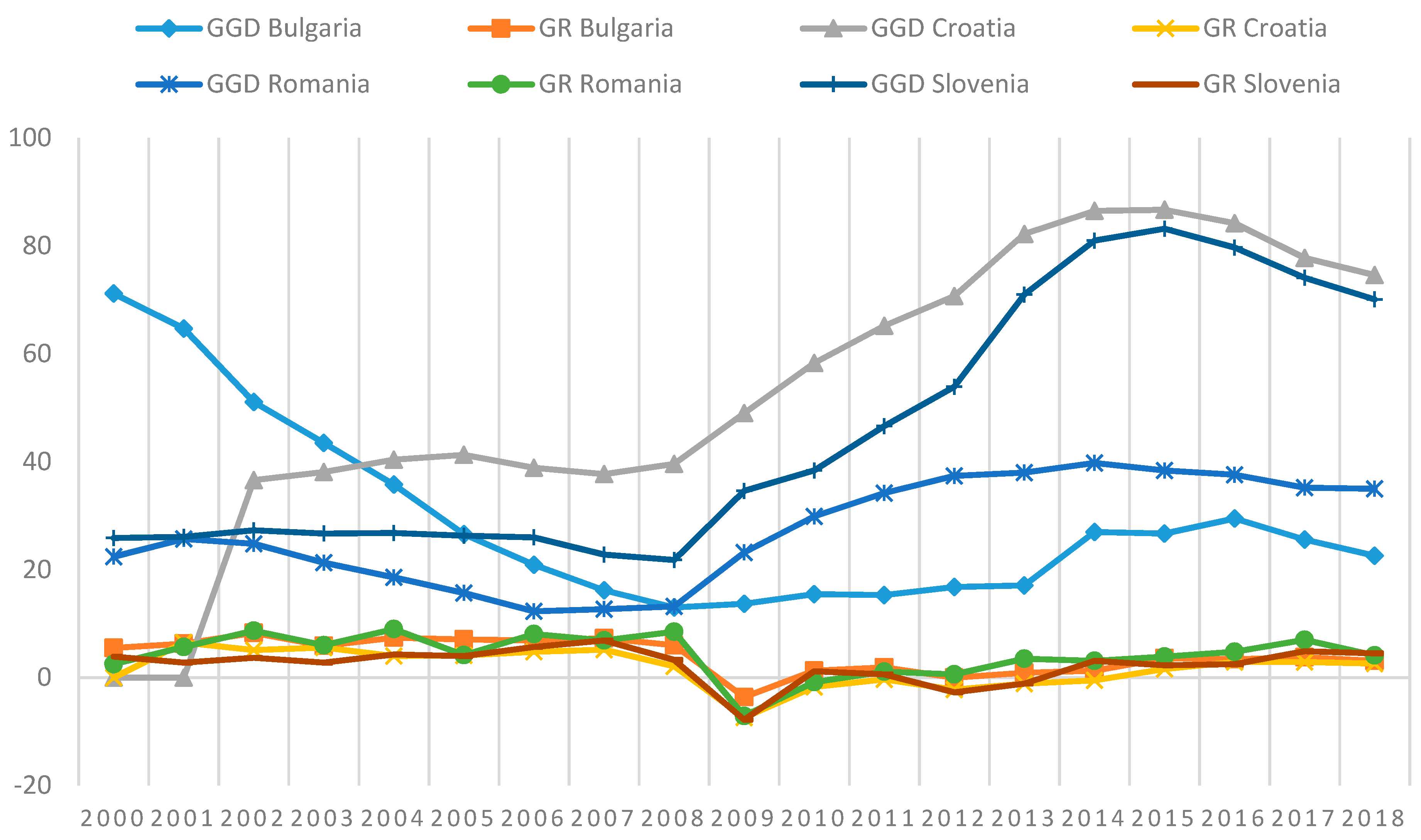
Within the four EU Balkan countries, GGD and GD as a percentage of GDP illustrated some volatility over the nineteen-year study (Table 3). Bulgaria, from 2003 onward, and Romania, throughout the whole study period, demonstrated two of the lowest GGDs EU-wide, with very dynamic growth rates throughout 2002–2008. They both experienced low growth from the recession in 2009, in which Bulgaria rose to above 3% from 2015 onward while Romania did not (Figure 6). Bulgaria’s GD was under control with the exception of when it grew up to 3% of GDP in the years of 2009–2010 and 2014. Romania’s GD remained above 3% in 2000–2001 and 2008–2012 (Figure 7). Bulgaria recorded a few years and minimal amount of government surplus, while Romania none.
The GGD in Croatia demonstrated a tendency to grow. The growth rate was dynamic from 2001–2007, after which an inversion occurs in which GGD was above the recommended level in 2011–2018 (Figure 6). The country had a problem with GD throughout the considered period with the exception of 2006–2007 and, more recently, 2016–2018 (Figure 7). The growth rate was slightly slow during the recession period of 2009–2014.
In 2000–2012, Slovenia had a low GGD before it began to grow above the recommended 60% of GDP (Figure 6). Its economic growth rate shows a dynamic fluctuation between 2000 and 2008, recession in 2009 and 2012–2013, and then growth from 2013 onward. Its GD was problematic in 2001 and from 2008–2014, with 2013 recording the worst GD result (i.e., −15.0%) study-wide (Figure 7). In summary, the Balkan countries experienced low levels of GGD and GD, allowing them to record a dynamic economic growth rate with the exception of the financial crisis period of 2009.
5. Discussion
5.1. Tax System Evaluation
An evaluation of the varying tax systems from each of the eleven EU MSs were assessed to further understand comparability and best practices. Two tax baseline indicators were considered in order to identify and better characterize how each MS acquires state-level finance (i.e., total general government revenue (GGR) and total tax and contribution rate of profit). First, an examination of the total GGR as a percentage of GDP was looked at between 2000 and 2018 (Table 4). Over the nineteen-year period, within the Baltic countries, total GGR mostly remained under 40%, with few exceptions apart from Latvia, which increased after the financial crisis of 2008 to 48.8% in 2014 and 44.7% in 2018. For Central and Eastern European countries, GGR as a percentage of GDP was generally moderate apart from the particular case of Hungary. Over the entire nineteen-year period, Hungary consistently implemented some of, and if not, the highest GGR rates of any post-communist EU MS. Hungary’s economic policy is reflective of high spending and poor fiscal management. In the case of the Balkan countries, overall, there was a distinct split between Bulgaria and Romania (i.e., two former independent communist countries) and Croatia and Slovenia (i.e., two internal former parts of Yugoslavia). Bulgaria and Romania are distinctly characterized as countries with low GGR rates, with Romania having the lowest of any country study-wide. By contract, the two ex-Yugoslavian MSs imposed inverse schemes by having some of the highest GGR rates, after Hungary, in comparison to the rest of the countries studied. In all, a generalization of the total GGR as a percentage of GDP for all of the post-communist EU MSs indicated lower rates in the north and east, mid-levels in the center, and higher in the south.
Second, a contemporary assessment of restrictive fiscal policy was compared using the indicator of total tax and contribution rate (i.e., all taxes and contributions from the private sector) as a percentage of profit in 2018 (Figure 8). The mean tax rate for the all countries was 38.5%. The Baltic and Central and Eastern European countries as well as Romania showed somewhat high private sector tax and contribution rates above 40%, with the exception of Latvia at 36.0%. Slovakia and Estonia sported particularly higher rates at 49.7% and 48.7%, respectively. These higher rates are better suited toward the Baltic countries and the Czech Republic due to fiscal policy stability and simplicity. In the Balkan countries, with the exception of Romania, we found the lowest rates of total tax and contribution from all private sector entities. Croatia sported the lowest rate, study-wide, at 20.5%, which is reflective of a high shadow-economy that parallels other ex-Yugoslavian non-EU MSs (Medina and Schneider 2018). As such, low levels indicate poor repayment financing of GDD and GD. In reflection, exploratory findings throughout the three regional blocks point toward the importance of developing effective taxation systems that are simple in structure, minimally reformed once a target level is achieved and, as a general rule, low. Recommendations would include building stable taxation that citizenry and the private sector feel is fair to accommodate inflows.
5.2. Conditions of Public Finance
Within the EU, the fiscal policy of GGD and GD is regulated and controlled under the law. EU MSs are required to respect their level of GGD and GD under the press of European institutional restrictions. This research is integral in effectively developing and adding a knowledge base within the EU’s public finance continuum and at the international level in reporting on and adding to MSs’ economic profiles. As such, a noteworthy concern is when government finance becomes excessively elevated (i.e., high GGD and GD), thereby reinforcing a need for economic policy reform of government income and expenditure. As governments continue to look for and experiment with optimal fiscal policy on how to improve and influence citizenry and the private sector, there is an important need in understanding the essence of GGD- and GD-related approaches developed to deal with these problems. At present, since economies are measured and evaluated by economic growth rate, the interdependency with GGD and GD interlaces the importance of government finance decision making. One can hypothesize public finance level in relation to GGD and GD as directly influencing economic growth. This idea expounds problems of fiscal policy and challenges a number of economic theories—specifically Keynesian theory, Ricardian theory and, to some degree, the theory of supply. As such, we treat GGD and GD as a negative problem which needs reactionary resolve via knowledgeable economic reform and policy. Explaining this viewpoint elucidates the stance and position on how potential policy recommendations can be put forth.
The idea of researching post-communist EU MSs plays on the fact that all these countries experienced, to some degree, specific transformative processes after communism and, again, with European enlargement. Three distinct transformative states exist, namely: former Soviet Union countries (i.e., Estonia, Latvia, and Lithuania), former independent communist countries that remain intact today (i.e., Poland, Hungary, Romania, and Bulgaria) and former larger communist countries that are now smaller ones (i.e., Czechoslovakia that became the Czech Republic and Slovakia, and Yugoslavia that became six countries in which only Croatia and Slovenia are EU MSs). This histo-geographical analysis is stimulating since we find the former Soviet Union countries are the only core group of countries that match this study’s regional groupings (i.e., blocks). With this in mind, a comparative examination of GGD, GD, and growth rate clearly illustrates the Baltic countries are faring best. We can infer these results are not related to being a part of the ex-Soviet Union but rather due to being relatively small in size, small in population, homogeneous, entrepreneurial, free market-friendly, noncorrupt, with a high level and regard for the law, highly educative, as well as with high levels of infrastructure throughout the three countries. The Baltic countries as a block are often noted as supportive of each other with strong infrastructural ties, which relates to a triad of economic policy that is liberal market-oriented. However, it should be stated, GGD, GD, and growth rate were generally stable in all countries—with the exceptions of Hungary, Croatia, and Slovenia. In all, negative or stagnant periods throughout the study often revealed a positive trend when digging a little deeper at the country profile level. On a wider scale, it was evident that the world financial crisis of 2008 had a deteriorative impact on growth rate on all countries—especially from 2009. The latter years of the study period presented promising findings in which a precedent amount of data gave signal to a rebirthing of stability and public finance in all MSs.
To better cognize the avoidance of problems with GGD and GD, there needs to be an open, effective free market economy. In theorizing this requisite, the need to build an equal or surplus central budget that decreases GGD is crucial. Additionally, each government should consider savings in State expenditures as well as preparing itself (i.e., internationally, nationally, and locally) to best deal with public finance crises or economic slowdown. Possible reactive securities and safety net approaches would be beneficial. A key advantage to dealing with the problems of fiscal policy is first recognizing the issues at hand and piecing together the reporting. As such, dataset collection is an important piece of the puzzle and useful tool in developing effective best practices via historical reporting. Since the problem within all post-communist EU MSs is short in comparison to Western Europe and North America, these countries have had to transform and absorb very quickly (i.e., liberal free market economics) in the past three decades. Trend-based approaches offer an immediate snapshot of what has worked versus not, consequently making it easier to manage and control GGD and GD in the future.
6. Conclusions
The reporting conducted on all eleven post-communist EU MSs, over the nineteen-year period of 2000–2018, on GGD and GD reveals a number of influencing factors relating to economic growth. The research examined different types of GGD and GD, with emphasis on MSs’ economy and government fiscal policy. It is evident that GGD and GD increase as a result of State intervention by reacting to economic fluctuations needed in fashioning more efficient fiscal policy initiatives. The data created by this study exemplify how Eurostat statistics are vital to EU progress, knowhow, and transparency. Negative or stagnant periods throughout the study revealed a general positive trend over the long term. Unmistakably, the world financial crisis of 2008 had a somewhat detrimental effect on all MSs—with some arguing Poland’s exemption. In the latter years of the data, economic promise signaled high potential for renewed public finance and stability-oriented initiatives. It was found that GGD and GD are interlaced with public finance and fundamentally influence economic growth, particularly via investment. As such, high GGD and GD can put significant pressure on economic success. The evaluation on tax systems summarizes an interwoven block-oriented scope; that is, the Baltic countries can be considered as having lower rates of total GGR as a percentage of GDP, Central and Eastern European countries mid-level rates, and the Balkan countries higher—noting a number of exemptions to this generalization.
Additional inquiries should examine tools that best alleviate GGD and GD by associating negative influences with political, historical, and traditional or cultural factors. Unfortunately, a few disadvantages of the research restricted us to using only one economic factor to interconnect with GGD and GD (i.e., economic growth rate). To improve the study, increasing the use of variables, Eurostat parameters, and overall macroeconomic data could be beneficial. Supplementary indicators could include GDP per capita, unemployment, rate of investments, rate of exchange (i.e., stable or not), and balance of payments. By adding additional indicators, a more objective and distinct evaluation of the potential influence of GGD and GD on the economy could be achieved.
Furthermore, the analyzing period could also be spread over a longer period of time, including updated annual reporting. Enlarging the study with the rest of the EU could also be undertaken, with comparative East–West differences in GGD and GD with important findings relating to GDP. As such, it would be interesting to comparatively examine the more successful and stronger market economies from Western Europe which would, inferentially, immediately move the study’s goalposts in a more competitive direction.
Author Contributions
Conceptualization, Data curation, A.P.; Methodology, Software, Validation, Formal analysis and Writing—Original Draft preparation, A.P. and G.T.C.; Investigation, Resources, Writing—Review and Editing, A.P., S.T.A., and G.T.C.; Visualization and Supervision, Project administration, and Funding acquisition, G.T.C.
Funding
This research received no external funding.
Conflicts of Interest
The authors declare no conflict of interest.
References
- Agénor, Pierre-Richard, and Peter J. Montiel. 2005. Development Macroeconomics, 4th ed. Princeton: Princeton University Press, ISBN 9780691165394. [Google Scholar]
- Alaimo, Katherine, Elizabeth Packnett, Richard A. Miles, and Daniel J. Kruger. 2008. Fruit and Vegetable Intake among Urban Community Gardeners. Journal of Nutrition Education and Behavior 40: 94–101. [Google Scholar] [CrossRef] [PubMed]
- Alesina, Alberto, and Silvia Ardagna. 1998. Tales of Fiscal Adjustment. Economic Policy 13: 487–545. [Google Scholar] [CrossRef]
- Altiparmakov, Nikola. 2018. Another Look at Causes and Consequences of Pension Privatization Reform Reversals in Eastern Europe. Journal of European Social Policy 28: 224–41. [Google Scholar] [CrossRef]
- Ardagna, Silvia. 2004. Fiscal Stabilizations: When Do They Work and Why. European Economic Review 48: 1047–74. [Google Scholar] [CrossRef]
- Ari, Ibrahim, Muammer Koc, Ibrahim Ari, and Muammer Koc. 2018. Sustainable Financing for Sustainable Development: Understanding the Interrelations between Public Investment and Sovereign Debt. Sustainability 10: 3901. [Google Scholar] [CrossRef]
- Ball, Laurence, and Nicholas Gregory Mankiw. 1995. What Do Budget Deficits Do? Cambridge: National Bureau of Economic Research. [Google Scholar] [CrossRef]
- Barro, Robert. 1988. The Ricardian Approach to Budget Deficits. Cambridge: National Bureau of Economic Research. [Google Scholar] [CrossRef]
- Barro, Robert J., and Xavier Sala-i-Martin. 2004. Economic Growth. Cambridge: MIT Press, ISBN 9780262025539. [Google Scholar]
- Brzozowski, Michał, Paweł Gierałtowski, Dominika Milczarek, and Joanna Siwińska-Gorzelak. 2006. Instytucje a Polityka Makroekonomiczna i Wzrost Gospodarczy. Warsaw: Uniwersytet Warszawski. [Google Scholar]
- Clements, Benedict, Rina Bhattacharya, and Toan Quoc Nguyen. 2003. External Debt, Public Investment, and Growth in Low-Income Countries. IMF Working Paper Number 03/249. Washington, DC, USA: Fiscal Affairs Department, International Monetary Fund. [Google Scholar]
- Compant, Stéphane, Birgit Reiter, Angela Sessitsch, Jerzy Nowak, Christophe Clément, and Essaïd Ait Barka. 2005. Endophytic Colonization of Vitis vinifera L. by Plant Growth-Promoting Bacterium Burkholderia Sp. Strain PsJN. Applied and Environmental Microbiology 71: 1685–93. [Google Scholar] [CrossRef] [PubMed]
- Ćwikliński, Henryk. 2004. Polityka Gospodarcza. Gdańsk: Wydawnictwo Uniwersytetu Gdańskiego, ISBN 83-7326-233-4. [Google Scholar]
- Deshpande, Ashwini. 1997. The Debt Overhang and the Disincentive to Invest. Journal of Development Economics 52: 169–87. [Google Scholar] [CrossRef]
- Dzwonkowski, Henryk. 2013. Deficyt i Dług Publiczny. Łódz: University of Łódz Lecture Series. [Google Scholar]
- Eaton, Jonathan. 1993. Sovereign Debt: A Primer. The World Bank Economic Review 7: 137–72. [Google Scholar] [CrossRef]
- European Council. 1997. Resolution of the European Council on the Stability and Growth Pact Amsterdam, 17 June 1997. Amsterdam: European Council. [Google Scholar]
- Gaudemet, Paul Marie, and Joel Molinier. 2000. Finanse Publiczne. Warsaw: Polskie Wydawnictwo Ekonomiczne S.A., ISBN 83-208-1234-8. [Google Scholar]
- Giavazzi, Francesco, and Marco Pagano. 1990. Can Severe Fiscal Contractions Be Expansionary? Tales of Two Small European Countries. Cambridge: MIT Press. [Google Scholar] [CrossRef]
- Gradoń, Witold. 2003. Deficyt Budżetowy—Wybrane Problemy Interpretacyjne: Deficyt Budżetowy i Dlug Publiczny w Wybranych Krajach Europejskich. Białystok: Wyższa Szkoła Finansów i Zarządzania w Białymstoku. [Google Scholar]
- Hemming, Richard, Michael Kell, and Selma Mahfouz. 2002. The Effectiveness of Fiscal Policy in Stimulating Economic Activity: A Review of the Literature. Working Paper WP/02/208. Washington, DC: International Monetary Fund. [Google Scholar]
- Högenauer, Anna-Lena, and David Howarth. 2019. The Democratic Deficit and European Central Bank Crisis Monetary Policies. Maastricht Journal of European and Comparative Law. [Google Scholar] [CrossRef]
- Hyman, Richard. 2018. What Future for Industrial Relations in Europe? Employee Relations 40: 569–79. [Google Scholar] [CrossRef]
- Kim, Dong-Hyeon, Yu-Bo Suen, Shu-Chin Lin, and Joyce Hsieh. 2018. Government Size, Government Debt and Globalization. Applied Economics 50: 2792–803. [Google Scholar] [CrossRef]
- Kneller, Richard, Michael F. Bleaney, and Norman Gemmell. 1999. Fiscal Policy and Growth: Evidence from OECD Countries. Journal of Public Economics 74: 171–90. [Google Scholar] [CrossRef]
- Kosek-Wojnar, Maria, Stanisław Owsiak, and Krzysztof Surówka. 1994. Podstawy Teorii Finansów Publicznych. Cracow: Wyd. Akademia Ekonomiczna w Krakowie. [Google Scholar]
- Krugman, Paul. 1988. Financing vs. Forgiving a Debt Overhang. Journal of Development Economics 29: 253–68. [Google Scholar] [CrossRef]
- Łaszek, Aleksander. 2013. Metodologia Szacowania Długu Ukrytego. Warsaw: Forum Obywatelskiego Rozwoju. [Google Scholar]
- Lin, Shuanglin, and Kim Sosin. 2001. Foreign Debt and Economic Growth. The Economics of Transition 9: 635–55. [Google Scholar] [CrossRef]
- Marciniak, Stefana. 2013. Makro i Mikroekonomia. Warsaw: Wydawnictwo Naukowe PWN. [Google Scholar]
- Matarese, Valerie. 2013. Using Strategic, Critical Reading of Research Papers to Teach Scientific Writing: The Reading–research–writing Continuum. In Supporting Research Writing: Roles and Challenges in Multilingual Settings. Oxford: Chandos Publishing, pp. 73–89. [Google Scholar] [CrossRef]
- Medina, Leandro, and Friedrich Schneider. 2018. Shadow Economies Around the World: What Did We Learn Over the Last 20 Years? IMF Working Paper No. 18/17. Washington, DC, USA: International Monetary Fund. [Google Scholar] [CrossRef]
- Minea, Alexandru, and Patrick Villieu. 2010. Endogenous Growth, Government Debt and Budgetary Regimes: A Corrigendum. Journal of Macroeconomics 32: 709–11. [Google Scholar] [CrossRef]
- N’Zue, Felix Fofana. 2018. The Ivorian Debt: Should We Worry? Journal of Economics and International Finance 10: 11–21. [Google Scholar] [CrossRef]
- Neck, Reinhard, and Jan-Egbert Sturm. 2008. Sustainability of Public Debt. Cambridge: MIT Press. [Google Scholar]
- Neumann, Lilia, and Andrzej Paczoski. 2014. Wskaźniki Polityki Budżetowej Państw UE Wobec Paktu Stabilności i Wzrostu Oraz Ich Wpływ Na PKB per Capita. Polityka Gospodarcza 22: 73–77. [Google Scholar]
- OECD. 2013. Fiscal Federalism 2014. Paris: Organisation for Economic Co-operation and Development, ISBN 9789264204560. [Google Scholar] [CrossRef]
- OECD. 2017. Understanding Financial Accounts. Edited by Peter van de Ven and Daniele Fano. Paris: Organisation for Economic Co-operation and Development. [Google Scholar] [CrossRef]
- Ortiz-Rodríguez, David, Andrés Navarro-Galera, and Francisco J. Alcaraz-Quiles. 2018. The Influence of Administrative Culture on Sustainability Transparency in European Local Governments. Administration & Society 50: 555–94. [Google Scholar] [CrossRef]
- Pattollo, Catherine, Hélène Poirson, and Luca Antonio Ricci. 2011. External Debt and Growth. Review of Economics and Institutions 2. [Google Scholar] [CrossRef]
- Pegkas, Panagiotis. 2018. The Effect of Government Debt and Other Determinants on Economic Growth: The Greek Experience. Economies 6: 10. [Google Scholar] [CrossRef]
- Renear, Allen H., and Carole L. Palmer. 2009. Strategic Reading, Ontologies, and the Future of Scientific Publishing. Science 325: 828–32. [Google Scholar] [CrossRef] [PubMed]
- Romer, David, Adam Szeworski, and Andrzej Malawski. 2000. Makroekonomia Dla Zaawansowanych. Warsaw: Wydawnictwo Naukowe PWN. [Google Scholar]
- Saint-Paul, Gilles. 1992. Fiscal Policy in an Endogenous Growth Model. The Quarterly Journal of Economics 107: 1243–59. [Google Scholar] [CrossRef]
- Serven, Luis. 1997. Uncertainty, Instability, and Irreversible Investment: Theory, Evidence, and Lessons for Africa. Policy Research Working Paper Series; Washington, DC: World Bank. [Google Scholar]
- Shah, Mohammad Aminur Rahman, Anisur Rahman, and Sanaul Huq Chowdhury. 2017. Sustainability Assessment of Flood Mitigation Projects: An Innovative Decision Support Framework. International Journal of Disaster Risk Reduction 23: 53–61. [Google Scholar] [CrossRef]
- Smyth, David J., and Yu Hsing. 1995. In Search Of An Optimal Debt Ratio For Economic Growth. Contemporary Economic Policy 13: 51–59. [Google Scholar] [CrossRef]
- Tobera, Paweł. 2013. Dług Publiczny—Istota, Przyczyny Powstania, Instrumenty Finansowania: Ludzie, Zarządzanie, Gospodarka. Miscellanea Oeconomicae: Studia i Materiały 1: 428–29. [Google Scholar]
- Van Der Veer, Reinout A., and Markus Haverland. 2018. Bread and Butter or Bread and Circuses? Politicisation and the European Commission in the European Semester. European Union Politics 19: 524–45. [Google Scholar] [CrossRef] [PubMed]
- Wernik, Andrzej. 2001. Deficyty Budżetowe i Metody Ich Liczenia. Biuro Studiów i Ekspertyz, Kancelaria Sejmu 239: 5–8. [Google Scholar]
- Wiśniewski, Jan. 2015. Budget Deficit and Government Debt as Major Challenges to Public Finance in Today’s Economy. Prace Naukowe Wyższej Szkoły Bankowej w Gdańsku 39: 17–25. [Google Scholar]
- Yang, Lu, Jason Ma, Shigeyuki Hamori, Lu Yang, Jason Z. Ma, and Shigeyuki Hamori. 2018. Dependence Structures and Systemic Risk of Government Securities Markets in Central and Eastern Europe: A CoVaR-Copula Approach. Sustainability 10: 324. [Google Scholar] [CrossRef]
Figure 1.
Map of the study area with defined regional blocks and relating European Union Member States.
Figure 1.
Map of the study area with defined regional blocks and relating European Union Member States.

Figure 2.
The Baltic countries’ GGD percentage of GDP versus growth rate percentage change from previous year, 2000–2018; Source: Eurostat.
Figure 2.
The Baltic countries’ GGD percentage of GDP versus growth rate percentage change from previous year, 2000–2018; Source: Eurostat.

Figure 3.
The Baltic countries’ GD percentage of GDP versus growth rate percentage change from previous year, 2000–2018; Source: Eurostat.
Figure 3.
The Baltic countries’ GD percentage of GDP versus growth rate percentage change from previous year, 2000–2018; Source: Eurostat.

Figure 4.
Central and Eastern European countries’ GGD percentage of GDP versus growth rate percentage change from previous year, 2000–2018; Source: Eurostat.
Figure 4.
Central and Eastern European countries’ GGD percentage of GDP versus growth rate percentage change from previous year, 2000–2018; Source: Eurostat.

Figure 5.
Central and Eastern European countries’ GD percentage of GDP versus growth rate percentage change from previous year, 2000–2018; Source: Eurostat.
Figure 5.
Central and Eastern European countries’ GD percentage of GDP versus growth rate percentage change from previous year, 2000–2018; Source: Eurostat.

Figure 6.
The Balkan countries’ GGD percentage of GDP versus growth rate percentage change from previous year, 2000–2018; Source: Eurostat.
Figure 6.
The Balkan countries’ GGD percentage of GDP versus growth rate percentage change from previous year, 2000–2018; Source: Eurostat.

Figure 7.
The Balkan countries’ GD percentage of GDP versus growth rate percentage change from previous year, 2000–2018; Source: Eurostat.
Figure 7.
The Balkan countries’ GD percentage of GDP versus growth rate percentage change from previous year, 2000–2018; Source: Eurostat.

Figure 8.
Total tax and contribution rate as a percentage of profit in post-communist EU MSs in 2018; Source: The World Bank.
Figure 8.
Total tax and contribution rate as a percentage of profit in post-communist EU MSs in 2018; Source: The World Bank.


Table 1.
The Baltic countries’ GGD percentage of GDP, GD percentage of GDP, and growth rate percentage change from previous year, 2000–2018.
Table 1.
The Baltic countries’ GGD percentage of GDP, GD percentage of GDP, and growth rate percentage change from previous year, 2000–2018.
| Year | Estonia | Latvia | Lithuania | ||||||
|---|---|---|---|---|---|---|---|---|---|
| GGD | GD | GR | GGD | GD | GR | GGD | GD | GR | |
| 2000 | 5.1 | −0.1 | 9.9 | 12.1 | −2.7 | 5.3 | 23.5 | −3.2 | 3.6 |
| 2001 | 4.8 | 0.2 | 6.2 | 13.9 | −2.0 | 7.3 | 22.9 | −3.5 | 6.7 |
| 2002 | 5.7 | 0.4 | 6.2 | 13.2 | −2.2 | 7.1 | 22.1 | −1.9 | 6.8 |
| 2003 | 5.6 | 1.8 | 8.1 | 13.9 | −1.6 | 7.7 | 20.4 | −1.3 | 10.3 |
| 2004 | 5.1 | 2.4 | 6.2 | 14.3 | −1.0 | 8.8 | 18.7 | −1.4 | 7.4 |
| 2005 | 4.5 | 1.1 | 9.4 | 11.8 | −0.4 | 10.7 | 17.6 | −0.3 | 7.7 |
| 2006 | 4.4 | 2.9 | 10.3 | 9.9 | −0.6 | 11.9 | 17.2 | −0.3 | 7.4 |
| 2007 | 3.7 | 2.7 | 7.7 | 8.4 | −0.7 | 9.9 | 15.9 | −0.8 | 11.1 |
| 2008 | 4.5 | −2.7 | −5.4 | 18.7 | −4.1 | −3.6 | 14.6 | −3.1 | 2.6 |
| 2009 | 7.0 | −2.2 | −14.7 | 36.6 | −9.1 | −14.3 | 29.0 | −9.1 | −14.8 |
| 2010 | 6.6 | 0.2 | 2.3 | 47.5 | −8.5 | −3.8 | 36.2 | −6.9 | 1.6 |
| 2011 | 5.9 | 1.2 | 7.6 | 42.8 | −3.4 | 6.4 | 37.2 | −8.9 | 6.0 |
| 2012 | 9.5 | −0.3 | 4.3 | 41.4 | −0.8 | 4.0 | 39.8 | −3.1 | 3.8 |
| 2013 | 9.9 | −0.2 | 1.4 | 39.1 | −0.9 | 2.6 | 38.8 | −2.6 | 3.5 |
| 2014 | 10.4 | 0.8 | 2.8 | 40.8 | −1.6 | 2.1 | 40.7 | −0.7 | 3.5 |
| 2015 | 9.7 | 0.4 | 1.4 | 36.4 | −1.3 | 2.7 | 42.7 | −0.2 | 1.8 |
| 2016 | 9.5 | 0.3 | 1.6 | 40.1 | 0.0 | 2.0 | 40.2 | 0.3 | 2.3 |
| 2017 | 9.2 | −0.4 | 4.9 | 40.0 | −0.6 | 4.6 | 39.4 | 0.5 | 4.1 |
| 2018 | 8.4 | −0.6 | 3.9 | 35.9 | −1.0 | 4.8 | 34.2 | 0.7 | 3.5 |
Source: Eurostat.
Table 2.
Central and Eastern European countries’ GGD percentage of GDP, GD percentage of GDP, and growth rate percentage change from previous year, 2000–2018.
Table 2.
Central and Eastern European countries’ GGD percentage of GDP, GD percentage of GDP, and growth rate percentage change from previous year, 2000–2018.
| Year | Czech Republic | Hungary | Poland | Slovakia | ||||||||
|---|---|---|---|---|---|---|---|---|---|---|---|---|
| GGD | GD | GR | GGD | GD | GR | GGD | GD | GR | GGD | GD | GR | |
| 2000 | 17.0 | −3.5 | 4.2 | 55.1 | −3.0 | 4.2 | 36.5 | −3.0 | 4.3 | 49.6 | −12.0 | 1.4 |
| 2001 | 22.8 | −5.3 | 3.1 | 51.7 | −4.1 | 3.7 | 37.3 | −4.8 | 1.2 | 48.3 | −6.4 | 3.5 |
| 2002 | 25.9 | −6.3 | 2.1 | 55.0 | −8.9 | 4.5 | 41.8 | −4.8 | 1.4 | 42.9 | −8.1 | 4.6 |
| 2003 | 28.1 | −6.4 | 3.8 | 57.6 | −7.1 | 3.9 | 46.6 | −6.1 | 3.9 | 41.6 | −2.7 | 4.8 |
| 2004 | 28.5 | −2.7 | 4.7 | 58.5 | −6.4 | 4.8 | 45.3 | −5.1 | 5.3 | 40.6 | −2.3 | 5.1 |
| 2005 | 28.0 | −3.1 | 6.4 | 60.5 | −7.8 | 4.0 | 46.7 | −4.0 | 3.6 | 33.9 | −2.9 | 6.7 |
| 2006 | 27.9 | −2.3 | 6.9 | 64.7 | −9.3 | 3.9 | 47.2 | −3.6 | 6.2 | 30.8 | −3.6 | 8.5 |
| 2007 | 27.8 | −0.7 | 5.5 | 65.6 | −5.1 | 0.4 | 44.2 | −1.9 | 7.0 | 29.9 | −1.9 | 10.8 |
| 2008 | 28.7 | −2.1 | 2.7 | 71.6 | −3.6 | 0.9 | 46.6 | −3.6 | 4.2 | 28.2 | −2.3 | 5.6 |
| 2009 | 34.1 | −5.5 | −4.8 | 78.0 | −4.6 | −6.6 | 49.8 | −7.3 | 2.8 | 36.0 | −7.9 | −5.4 |
| 2010 | 38.2 | −4.4 | 2.3 | 80.6 | −4.5 | 0.7 | 53.3 | −7.5 | 3.6 | 40.8 | −7.5 | 5.0 |
| 2011 | 39.9 | −2.7 | 2.0 | 80.8 | −5.5 | 1.7 | 54.4 | −4.9 | 5.0 | 43.3 | −4.1 | 2.8 |
| 2012 | 44.7 | −3.9 | −0.8 | 78.3 | −2.3 | −1.6 | 54.0 | −3.7 | 1.6 | 52.4 | −4.3 | 1.7 |
| 2013 | 45.1 | −1.3 | −0.5 | 76.8 | −2.6 | 2.1 | 56.0 | −4.0 | 1.4 | 55.0 | −2.7 | 1.5 |
| 2014 | 42.7 | −1.9 | 2.7 | 76.2 | −2.3 | 4.0 | 50.5 | −3.3 | 3.3 | 53.9 | −2.7 | 2.6 |
| 2015 | 41.1 | −0.4 | 4.5 | 75.3 | −2.0 | 3.1 | 51.3 | −2.6 | 3.8 | 52.9 | −3.0 | 3.8 |
| 2016 | 37.2 | 0.6 | 2.4 | 74.1 | −1.8 | 2.0 | 54.4 | −2.4 | 2.7 | 51.9 | −1.7 | 3.3 |
| 2017 | 34.7 | 1.6 | 4.4 | 73.4 | −2.2 | 4.1 | 50.6 | −1.5 | 4.8 | 50.9 | −0.8 | 3.2 |
| 2018 | 32.7 | 0.9 | 2.9 | 70.8 | −2.2 | 4.9 | 48.9 | −0.4 | 5.1 | 48.9 | −0.7 | 4.1 |
Source: Eurostat.
Table 3.
The Balkan countries’ GGD percentage of GDP, GD percentage of GDP, and growth rate percentage change from previous year, 2000–2018.
Table 3.
The Balkan countries’ GGD percentage of GDP, GD percentage of GDP, and growth rate percentage change from previous year, 2000–2018.
| Year | Bulgaria | Croatia | Romania | Slovenia | ||||||||
|---|---|---|---|---|---|---|---|---|---|---|---|---|
| GGD | GD | GR | GGD | GD | GR | GGD | GD | GR | GGD | GD | GR | |
| 2000 | 71.2 | −0.5 | 5.5 | N/A | N/A | N/A | 22.4 | −4.6 | 2.5 | 25.9 | 3.6 | 3.9 |
| 2001 | 64.7 | 1.1 | 6.3 | N/A | N/A | 6.5 | 25.7 | −3.4 | 5.7 | 26.1 | −3.9 | 2.8 |
| 2002 | 51.1 | −1.2 | 8.3 | 36.6 | −3.5 | 5.1 | 24.8 | −1.9 | 8.7 | 27.3 | −2.4 | 3.7 |
| 2003 | 43.5 | −0.4 | 5.9 | 38.1 | −4.7 | 5.6 | 21.3 | −1.4 | 6.0 | 26.7 | −2.6 | 2.8 |
| 2004 | 35.8 | 1.8 | 7.4 | 40.4 | −5.2 | 4.0 | 18.6 | −1.1 | 9.0 | 26.8 | −2.0 | 4.3 |
| 2005 | 26.6 | 1.0 | 7.1 | 41.3 | −3.9 | 4.1 | 15.7 | −0.8 | 4.2 | 26.3 | −1.3 | 4.0 |
| 2006 | 20.9 | 1.8 | 6.9 | 38.9 | −3.4 | 4.8 | 12.3 | −2.1 | 8.1 | 26.0 | −1.2 | 5.7 |
| 2007 | 16.2 | 1.1 | 7.3 | 37.7 | −2.4 | 5.2 | 12.7 | −2.8 | 6.9 | 22.8 | −0.1 | 6.9 |
| 2008 | 13.0 | 1.6 | 6.0 | 39.6 | −2.8 | 2.1 | 13.2 | −5.5 | 8.5 | 21.8 | −1.4 | 3.3 |
| 2009 | 13.7 | −4.1 | −3.6 | 49.0 | −6.0 | −7.4 | 23.2 | −9.5 | −7.1 | 34.6 | −5.9 | −7.8 |
| 2010 | 15.5 | −3.2 | 1.3 | 58.3 | −6.2 | −1.7 | 29.9 | −6.9 | −0.8 | 38.4 | −5.6 | 1.2 |
| 2011 | 15.3 | −2.0 | 1.9 | 65.2 | −7.8 | −0.3 | 34.2 | −5.4 | 1.1 | 46.6 | −6.7 | 0.6 |
| 2012 | 16.8 | −0.3 | 0.0 | 70.7 | −5.3 | −2.2 | 37.4 | −3.7 | 0.6 | 53.9 | −4.1 | −2.7 |
| 2013 | 17.1 | −0.4 | 0.9 | 82.2 | −5.3 | −1.1 | 38.0 | −2.1 | 3.5 | 71.0 | −15.0 | −1.1 |
| 2014 | 27.0 | −5.4 | 1.3 | 86.5 | −5.5 | −0.5 | 39.8 | −0.9 | 3.1 | 81.0 | −5.0 | 3.1 |
| 2015 | 26.7 | −2.1 | 3.6 | 86.7 | −3.2 | 1.6 | 38.4 | −0.7 | 3.9 | 83.2 | −2.9 | 2.3 |
| 2016 | 29.5 | 0.0 | 3.4 | 84.2 | −0.8 | 2.9 | 37.6 | −3.0 | 4.8 | 79.7 | −1.8 | 2.5 |
| 2017 | 25.6 | 1.2 | 3.8 | 77.8 | 0.8 | 2.9 | 35.2 | −2.7 | 7.0 | 74.1 | 0.0 | 4.9 |
| 2018 | 22.6 | 2.0 | 3.1 | 74.6 | 0.2 | 2.6 | 35.0 | −3.0 | 4.1 | 70.1 | 0.7 | 4.5 |
Source: Eurostat 2019.
Table 4.
Total GGR as a percentage of GDP for all post-communist EU MSs, 2000–2018.
| Year | Baltic Countries | Central and Eastern European Countries | Balkan Countries | ||||||||
|---|---|---|---|---|---|---|---|---|---|---|---|
| Estonia | Latvia | Lithuania | Czech Rep | Hungary | Poland | Slovakia | Bulgaria | Croatia | Romania | Slovenia | |
| 2000 | 36.4 | 34.4 | 36.2 | 37.4 | 44.1 | 39.1 | 40.0 | 40.5 | N/A | 33.9 | 42.5 |
| 2001 | 35.0 | 35.3 | 33.6 | 37.7 | 43.1 | 40.3 | 38.0 | 42.0 | 43.7 | 32.9 | 43.1 |
| 2002 | 36.1 | 37.0 | 33.3 | 38.5 | 42.0 | 40.6 | 37.1 | 38.2 | 47.0 | 33.0 | 43.4 |
| 2003 | 35.2 | 40.5 | 32.3 | 42.5 | 41.9 | 39.7 | 37.2 | 38.5 | 45.2 | 32.9 | 43.2 |
| 2004 | 34.3 | 38.5 | 32.6 | 40.2 | 42.1 | 38.5 | 35.5 | 39.9 | 43.6 | 32.7 | 43.4 |
| 2005 | 34.0 | 39.3 | 33.7 | 39.3 | 41.6 | 40.4 | 36.9 | 38.1 | 43.0 | 32.7 | 43.6 |
| 2006 | 33.6 | 38.7 | 34.0 | 39.2 | 42.2 | 41.1 | 35.2 | 35.7 | 43.1 | 33.5 | 43.0 |
| 2007 | 34.1 | 37.6 | 34.4 | 39.7 | 44.8 | 41.4 | 34.4 | 38.8 | 43.0 | 34.7 | 42.1 |
| 2008 | 39.7 | 38.4 | 35.0 | 38.7 | 45.0 | 40.7 | 34.5 | 38.7 | 42.5 | 32.3 | 42.5 |
| 2009 | 46.1 | 42.1 | 35.8 | 38.7 | 45.9 | 37.8 | 36.3 | 35.3 | 42.3 | 30.3 | 42.4 |
| 2010 | 40.5 | 42.0 | 35.4 | 39.3 | 44.8 | 38.5 | 34.7 | 33.1 | 41.7 | 33.1 | 43.6 |
| 2011 | 37.4 | 42.3 | 33.5 | 40.3 | 44.1 | 39.1 | 36.5 | 31.9 | 40.6 | 34.1 | 43.3 |
| 2012 | 39.3 | 41.9 | 33.0 | 40.5 | 46.1 | 39.1 | 36.3 | 34.1 | 42.5 | 33.7 | 44.5 |
| 2013 | 38.5 | 41.9 | 32.9 | 41.4 | 46.7 | 38.5 | 38.7 | 37.3 | 42.4 | 33.3 | 44.8 |
| 2014 | 37.8 | 48.8 | 34.0 | 40.3 | 46.9 | 38.7 | 39.3 | 37.7 | 42.9 | 34.1 | 44.4 |
| 2015 | 39.6 | 40.6 | 34.6 | 41.1 | 48.2 | 39.0 | 42.5 | 38.8 | 45.2 | 35.4 | 44.9 |
| 2016 | 39.5 | 38.0 | 34.4 | 40.2 | 45.1 | 38.9 | 39.2 | 35.2 | 46.3 | 31.8 | 43.4 |
| 2017 | 39.3 | 37.4 | 33.6 | 40.5 | 44.7 | 39.7 | 39.4 | 36.2 | 46.1 | 30.9 | 43.2 |
| 2018 | 39.5 | 44.7 | 34.7 | 41.7 | 44.2 | 41.2 | 39.9 | 36.8 | 46.6 | 32.0 | 43.1 |
Source: Eurostat 2019.
© 2019 by the authors. Licensee MDPI, Basel, Switzerland. This article is an open access article distributed under the terms and conditions of the Creative Commons Attribution (CC BY) license (http://creativecommons.org/licenses/by/4.0/).
Share and Cite
MDPI and ACS Style
Paczoski, A.; Abebe, S.T.; Cirella, G.T. Debt and Deficit Growth Rate Reporting for Post-Communist European Union Member States. Soc. Sci. 2019, 8, 173. https://doi.org/10.3390/socsci8060173
AMA Style
Paczoski A, Abebe ST, Cirella GT. Debt and Deficit Growth Rate Reporting for Post-Communist European Union Member States. Social Sciences. 2019; 8(6):173. https://doi.org/10.3390/socsci8060173
Chicago/Turabian StylePaczoski, Andrzej, Solomon T. Abebe, and Giuseppe T. Cirella. 2019. "Debt and Deficit Growth Rate Reporting for Post-Communist European Union Member States" Social Sciences 8, no. 6: 173. https://doi.org/10.3390/socsci8060173
Note that from the first issue of 2016, this journal uses article numbers instead of page numbers. See further details here.