
Design and Analysis of an Active Disturbance Rejection Robust Adaptive Control System for Electromechanical Actuator


1
School of Energy and Power Engineering, Wuhan University of Technology, Wuhan 430036, China
2
Laboratory of Aerospace Servo Actuation and Transmission, Beihang University, Beijing 100191, China
*
Author to whom correspondence should be addressed.
Actuators 2021, 10(12), 307; https://doi.org/10.3390/act10120307
Submission received: 11 October 2021
/
Revised: 19 November 2021
/
Accepted: 21 November 2021
/
Published: 23 November 2021
(This article belongs to the Section Control Systems)
Abstract
:Airline electromechanical actuators (EMAs), on the task of controlling flight surfaces, hold a great promise with the development of more- and all-electric aircraft. Notwithstanding, the deficiencies in both robustness and adaptability of control algorithms prevent EMAs from extensive use. However, the state-of-the-art control schemes fail to precisely compensate the system nonlinear uncertainties of servo control. In this paper, from the innovation point of view, we tend to put forward the foundation of devising an active disturbance rejection robust adaptive control (ADRRAC) strategy, whose main purpose is to deal with the position servo control of EMA. Specifically, an adaptive control law is designed and deployed for resolving not only the nonlinear disturbance, but also the parameter uncertainties. In addition, an extended disturbance estimator is employed to estimate the external disturbance and thus eliminate its impact. The proposed controlling algorithm is deemed best able to address the external disturbance based on the nonlinear uncertainty compensation. With the input parameters and control commands, the ADRRAC strategy maintains servo system stability while approaching the controlling target. Following the algorithm description, a proof of the controlling stability of ADRRAC strategy is presented in detail as well. Experiments on a variety of tracking tasks are conducted on a prototype of an EMA to investigate the working performance of the proposed control strategy. The experimental outcomes are reported, which verify the effectiveness of the ADRRAC strategy, compared to widely applied control strategies. According to the data analysis results, our controller is capable of obtaining an even faster system response, a higher tracking accuracy and a more stable system state.
1. Introduction
Actuation systems for more electrical aircraft must balance requirements of high power, light weight, safety, fast response and continuity of service. The trend towards more- and all-electrical aircraft is gradually being accomplished with backup or substitute mechanical actuators with electric solutions [1]. As such, electromechanical actuators (EMAs) are considered as a leap forward and receive interest because of their higher efficiency and reduction in both weight and maintenance time compared with hydraulic actuators [2,3,4]. The famous Dreamliner, Boeing 787, employs EMAs in its landing gear braking and spoiler actuating [5]. Thereby, research remains ongoing to develop EMAs with better working performance.
While once restricted to working performance, employment of EMAs has greatly progressed with advances in control technology. In the context of permanent magnet synchronous motor studying, its position servo control during the work phase is most pronounced. The continuously increasing demand for control accuracy accelerates the devising and deploying of control strategies [6,7,8]. In line with the control strategy design process, research on EMAs focuses on the use of the state-of-the-art controllers. In industrial practice, conventional control strategies (i.e., PID control, fuzzy control, etc.), modern control strategies (sliding mode control, robust control, adaptive control, active disturbance rejection control, etc.) as well as their integration with intelligent algorithms, are employed for servo control in a variety of domains [9,10,11,12,13,14]. Specifically, Kumar and Rani reported a neural network-based adaptive control scheme in terms of position and force control, aiming to overcome the defects of the model-dependent controller via the intelligent techniques [15]. Furthermore, a synthesized controlling system, integrating proportion-integral-differential controller, H∞ controller and H∞ hybrid controller, is performed, which can favorably solve actual problems for the EMAs of spacecraft [16]. Gollapudi et al. introduced a way of driving four electromechanical actuation elements using an active fault-tolerance controller [17]. In addition, Wrat et al. applied a synthesized position control strategy to ensure the working performance under model uncertainties and dynamical load disturbance [18].
Notwithstanding, the applications of position servo control in EMA are still limited, basically due to its deficiency in high-robust control. In addition, control adaptability for uncertain and variable parameters is also a well-documented weakness of most control strategies. According to [19], strong robust control of uncertainties of an EMA on aircraft is critical for handling parameter perturbation and load disturbance. That is, an active disturbance rejection robust adaptive controller (ADRRAController) that robustly depends on the working properties of the position servo system has the potential to contribute to the evolution of EMAs.
This work starts with concentrating on the working principle of the position servo in EMA systems as well as its control law. Correspondingly, an active disturbance rejection robust adaptive control (ADRRAC) strategy is dedicatedly designed and deployed, targeting at addressing the position servo issues in EMA control. To this end, the nonlinear uncertainties of the system, together with their compensation, are integrated into the control strategy as well.
The rest of this paper is organized as follows: In Section 2, we introduce the background knowledge of position servo systems. Section 3 describes the system architecture of the RAC strategy. In Section 4, we explore the working performance achieved in the modeling and numerical simulation with the analysis of the controller. Finally, we conclude the research and describe some future work in Section 5.
2. EMA Architecture
A typical EMA system contains a mechanical actuation assembly, a controller and sensing elements. Distinctively, the mechanical actuation assembly is generally composed of mechanical components (such as a gearbox, lead screws, etc.) and a servo motor [20,21]. In general, EMAs are developed for flight control applications to drive a surface or an actuating component according to the control commands, as depicted schematically in Figure 1. The control commands, which can drive the motor to rotate forward and reverse, is the output of the controller [22,23]. In this instance, we take a classical planetary roller screw mechanism (PRSM) as the transmission component [24,25]. More details of PRSM are accessible in [26,27].
3. Proposed ADRRAC System for Position Servo Control
In terms of actuating, the nonlinearity and time-variation of EMAs can influence the system dynamics as well as the accuracy of servo control. This section introduces the architecture of the ADRRAC strategy and its working principle in detail. The system notations in the following description are presented in Table 1.
3.1. System Modeling
The mathematical modeling of EMA is established already. Let represent the basic system parameters of EMA. We thus have:
Notably, Equation (1) indicates the transmission of PRSM, which transforms the rotation to linear displacement. Further, the relationship between the electromagnetic torque and the current of the motor is given in Equation (2). In such a manner, the PRS is driven by the motor operation. Both and are unknown variables. The former ranges from 0 to the maximum output, and the latter can be estimated via adaptive control [28,29]. The motor dynamics are performed using both the voltage and the current of motor, as presented in Equation (3).
To facilitate the controller design, we shall re-define the system parameters as:
From Equations (5) and (6), we have , , , and . In addition, represents the external load of the system. In this way, the EMA model is performed for further processing.
3.2. Projection Mapping
At this stage, we employ the projection mapping before the controller deployment, which is computationally efficient to work with. Formally, is the estimation of whilst is the estimation error. Their relationship is conveyed as:
Specifically, the parametric adaptive law will be synthesized for . In ADRRAC strategy, is selected as the adaptive parameter due to its functioning as the damping of the controller [30]. As such, is applied to regulate the controlling precision in tracking cases.
A typical is defined as th component of vector . The projection, which is a discrete function, is presented in Equation (8):
As expected, , representing the adaptation law, is able to comply with the following condition:
where stands for a gain matrix and represents an adaptative control matrix.
3.3. Control Strategy Establishment
Seeing that the external load is an unknown variable, an extended disturbance estimator (EDE) is proposed to facilitate the computation. In line with the EMA model, we have:
together with
where stands for the gain of EDE.
We tend to set the control command as a given input of the system displacement The closer approaches , the higher accuracy the controller obtains. The control objective is to get an output tracking error equaling 0, as shown in Equation (12).
For , we can derive:
Suppose that
with
Only if , can we derive . In this way, the system error can be determined.
For , we can also deliver the dynamics of as:
Similarly, we define
where is taken as a virtual input variable. To support the resolution of , we also introduce two more parameters, namely and .
where
and
Consequently, Equation (16) is re-written as:
where , and .
Based on Equation (20), we can get via Equation (22) as well:
where is given as:
with
and
Substantially, we have:
where and stand for the calculable and incalculable component of , respectively. With such a definition, seeing that is a parameter with respect to time, the calculable part , based on partial differential, can be expressed as:
Correspondingly, the incalculable part resolved by the robust term is:
In line with this procedure, it is clear that can also be transformed to:
where .
According to the working principle of EDE, we now define the observer error as:
Similarly, for other system parameters, the observer errors can be:
and
On this occasion, the vector is taken to characterize the system state. Then, the dynamics of the observer error are performed as:
where , and .
The diagram of the proposed control strategy is exhibited in Figure 2 based on the above devising.
3.4. Main Results
The purpose for controlling is that all closed loop system signals are bounded while asymptotic output tracking can be achieved [30]. To this end, we primarily carry out a Lyapunov candidate [31] to investigate the system stability. Firstly, a matrix is introduced, which satisfies:
For , the Lyapunov function is written as:
Then the time derivate of is given as:
Conforming to Equation (34) as well as the parameter properties, falls into:
Based on the adaptive control law of ADRRAC, we have:
In this case, the upper bound of is revised to:
with
where and .
On the other hand, for , the corresponding Lyapunov function is performed, i.e.,
in relation to and , Equation (40) is revised to:
As such, the time derivate of satisfies:
Let
and is arbitrary big. Thus, is derived from:
By defining and , we thus have:
According to Equation (44), is bounded by:
where . In this way, the system can achieve asymptotic stability.
4. Experiments
4.1. Experimental Setup
In order to verify the technical efficacy of the proposed control strategy, the test rig is built up. Fundamental experiments are conducted to demonstrate the working performance of the EMA system. The hardware architecture is presented in Figure 3 while the test rig together with the experimental components is illustrated in Figure 4.
In terms of this experiment, a U30720A AC servo motor is employed for EMA driving, whose no-load rotating speed is 1500 r/min and the torque constant is 3.61 N·m/A. The PRS in the EMA has a maximum static output of 116,400 N and a continuous output of 17,800 N. The intrusion detection of the cylinder displacement conducted [32,33], which employs the GEL235 Multi-turn type absolute encoder from Lenord, Bauer & Co. [34]. The signal detector and controller are integrated into one industrial computer with different A/D and D/A cards installed. Both cards are of 16 bits. Control commands are generated on the host computer beforehand with a sampling rate of 200 Hz. Subsequently, reference inputs are sent to the motor of the EMA via the transfer of the controller in real time [35]. According to the control commands, the EMA can be operated in distinctive working mode. Meanwhile, the position information of the cylinder is delivered as the system feedback to the control strategy by the signal detecting component. In this way, the controller output can be regulated.
4.2. Result Analysis
In the task of performing the ADRRAC for EMA position servo control, we take two other comparative control strategies, which are PID (Proportional Integral Derivative) control and ARC (Adaptive Robust Control). In practical use, the former is of high robustness and high reliability [36,37] while the latter is known for its stability and accuracy [38,39]. Specifically, the Ziegler-Nichols tuning method is applied to the PID controller for parameter tuning, based on which to reduce the oscillation and improve the robustness [40]. With a 200 N external load applied in advance, four sets of comparative tests are conducted:
- (1)
- A position reference of 0.2 Hz sinusoidal signal is employed to verify the tracking performance.
- (2)
- A position reference of 1 Hz sinusoidal signal is employed to evaluate the tracking performance.
- (3)
- A position reference of 1 Hz sinusoidal signal with a disturbance of at 2 s is employed to evaluate the robustness.
- (4)
- A position reference of 10 mm step signal is employed to verify the tracking performance.
The results of the first evaluation set are shown in Figure 5, Figure 6 and Figure 7. It is obvious that the proposed control strategy outperforms other controllers in low-frequency signal tracking. There is a substantial gap between the position error of the ADRRAC strategy and the other two. Following the reference control command, the error of the proposed controller is restricted to the range of . The main reason for this is due to the application of the adaptive control law. The ADRRAC strategy shows its superiority in system compensation in spite of the external load disturbance.
Similarly, in terms of the reference input with 1 Hz frequency, ADRRAC is still the best-performing model. The outcomes of the 1 Hz sinusoidal signal of the three control strategies are presented in Figure 8, Figure 9 and Figure 10. Although the tracking error increases with the increasing of control frequency, the position error of ADRRAC, compared to other baseline controllers, kept within 0.000161 m. In contrast, the maximum error for PID and ARC are 0.000778 m and 0.000438 m, respectively. Clearly, the proposed controller is a better alternative to the classical control strategies. The adaptive law provides a more stable response in system tracking. Since our controller is more accurate and more capable in dealing with the nonlinear disturbance, it is reasonable to expect better robustness against external uncertainties and thus better performance, as is the case.
To further investigate the robustness of ADRRAC strategy, a 700 N external disturbance is applied to the three controllers during the tracking of sinusoidal signal. When the EMA moves in the forward and backward direction, the system responses of different control strategies with respect to time are presented in Figure 11, Figure 12 and Figure 13. According to Figure 11, in line with the disturbance, the position error of PID control strategy reaches 0.0673 m and fluctuates within this value. The fluctuation of PID controller lasts until the end of the test. For the ARC strategy, the error rises to 0.0336 m at first and then decreased to nearly 0.01 m gradually (Figure 12). By contrast, our controller has a 0.0155 m tracking error with the disturbance implementing (Figure 13). Subsequently, the error is suppressed and drops to 0 within a short time. In such a way, the system stays stable and retains a consistent response. More indicators to demonstrate the control performance are given in Table 2. We generally take absolute peak value, average value and standard deviation of the 1 Hz sinusoidal input tracking errors. Notably, the outcome differences between ARC and ADRRAC are minor in the basic sinusoidal tracking task. The average error of ARC is even smaller than that of our controller. Furthermore, our controller can still maintain certain robustness to the external uncertainties as well as system parameter variation during a disturbance. The performance gaps between ADRRAC and ARC are 0.0145 for the average error and 0.0181 for the peak error, which are significant.
Based on the results in Figure 13, it can be observed that the robust item, together with the EDE, is capable of eliminating the tracking error and shortening the settling time. Specifically, the estimation of external disturbance of the EDE is presented in Figure 14. In addition, by exploiting the EDE in ADRRAC, the involved parameters are regulated to adapt to the distinguishing inputs. The variation of five parameters in our controller is exhibited in Figure 15. One can easily see that all these parameters vary conforming to the external disturbance. According to Figure 15 and Figure 16, during the performing of control strategy, the parameter estimation involves not just the external impacts, but also the parameter adaption. Distinctively, the large gradually converges to its initial value with the application of ; and pulse to the disturbance and stabilized in different values; and oscillate around the output and further preserve constant within 0.2 s. As such, all the parameters in our controller adapt to a compromise to reduce the tracking error and optimize the disturbance estimation. With the joint effect of the parameters, the ADRRAC strategy outperforms other baseline methods in maintaining the system stability and obtaining a faster response.
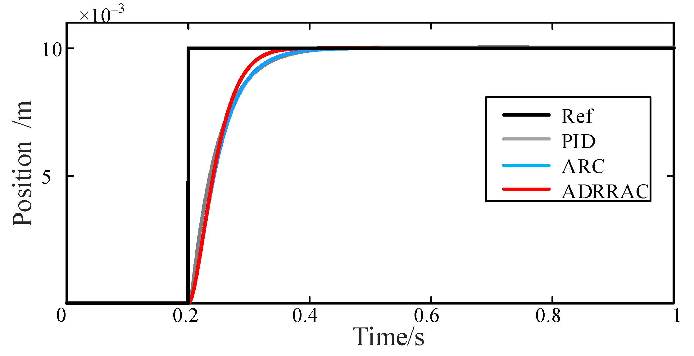
In addition to the sinusoidal signal tracking task, a step command experiment is also conducted. The tracking performance of the four controllers is presented in Figure 16. Notably, all these controllers have no overshoots due to the small inertia of EMA system. For system rapidity description, our controller has the fastest response with the settling time of 3.67 s. Compared to the PID and ARC strategy, the proposed ADRRAC strategy still obtains a better result in step signal tracking.
Based on the experimental results above, we thus conclude that the proposed control strategy, performing compensations for the external uncertainties, is effective in precisely tracking with respect to servo control in EMA systems.
5. Conclusions
In this work, a robust adaptive control for position servo control for an electro-mechanical actuator operation is established. During the devising process, the adaptive control law is integrated with the nonlinear controller, in which way the parametric uncertainties and unmodeled disturbances can be addressed. Further, the application of the EDE is capable of estimating the external disturbance and maintaining the system reliability. The proof of controlling stability indicates that the ADRRAC strategy can effectively reduce the integration difficulties between parametric-adaptive based and disturbance-based control. Experimental results verify the technical efficacy of ADRRAC strategy. In comparison to the baseline controllers, our method shows its distinctiveness in tracking accuracy. Specifically, the use of the adaptive control law together with the EDE results in an even better working performance in dealing with system uncertainties. For the task of position servo control, the proposed control strategy is taken as the best alternative when tacking the nonlinear external disturbance.
Author Contributions
Conceptualization, Q.C., H.C., D.Z. and L.L.; methodology, L.L. and Q.C.; software, L.L. and H.C.; validation, D.Z.; formal analysis, Q.C.; investigation, H.C.; resources, D.Z.; data curation, L.L. and Q.C.; writing—original draft preparation, L.L. and H.C.; writing—review and editing, L.L., Q.C. and D.Z.; visualization, L.L. and H.C.; supervision, H.C., Q.C. and D.Z.; project administration, H.C. All authors have read and agreed to the published version of the manuscript.
Funding
No fundings of this work.
Institutional Review Board Statement
Not applicable.
Informed Consent Statement
Not applicable.
Data Availability Statement
Not available.
Conflicts of Interest
The authors declare no conflict of interest.
References
- Villani, M.; Tursini, M.; Fabri, G.; Castellini, L. Electromechanical actuator for helicopter rotor damper application. IEEE Trans. Ind. Appl. 2014, 50, 1007–1014. [Google Scholar] [CrossRef]
- Qiao, G.; Liu, G.; Shi, Z.; Wang, Y.; Ma, S.; Lim, T.C. A review of electromechanical actuators for More/All Electric aircraft systems. Proc. Inst. Mech. Eng. Part C J. Mech. Eng. Sci. 2018, 232, 4128–4151. [Google Scholar] [CrossRef] [Green Version]
- Koopmans, M.T.; Tumer, I.Y. Function-Based Analysis and Redesign of a Flyable Electromechanical Actuator Test Stand. In Proceedings of the ASME 2010 International Design Engineering Technical Conferences & Computers and Information in Engineering Conference, Montreal, QC, Canada, 15–18 August 2010; pp. 977–988. [Google Scholar]
- Woodburn, D.; Wu, T.; Zhou, L.; Hu, Y.; Lin, Y.-R.; Chow, L.; Leland, Q. High-Performance Electromechanical Actuator Dynamic Heat Generation Modeling. IEEE Trans. Aerosp. Electron. Syst. 2014, 50, 530–541. [Google Scholar] [CrossRef]
- Giangrande, P.; Galassini, A.; Papadopoulos, S.; Al-Timimy, A.; Calzo, G.L.; Degano, M.; Galea, M.; Gerada, C. Considerations on the Development of an Electric Drive for a Secondary Flight Control Electromechanical Actuator. IEEE Trans. Ind. Appl. 2019, 55, 3544–3554. [Google Scholar] [CrossRef]
- Manohar, G.A.; Vasu, V.; Srikanth, K. Development of a high redundancy actuator with direct driven linear electromechanical actuators for fault-tolerance. Procedia Comput. Sci. 2018, 133, 932–939. [Google Scholar] [CrossRef]
- Zhang, Q.; Zhou, C.; Xiong, N.; Qin, Y.; Li, X.; Huang, S. Multimodel-Based Incident Prediction and Risk Assessment in Dynamic Cybersecurity Protection for Industrial Control Systems. IEEE Trans. Syst. Man Cybern. Syst. 2015, 46, 1429–1444. [Google Scholar] [CrossRef]
- Fu, J.; Maré, J.-C.; Fu, Y. Modelling and simulation of flight control electromechanical actuators with special focus on model architecting, multidisciplinary effects and power flows. Chin. J. Aeronaut. 2017, 30, 47–65. [Google Scholar] [CrossRef] [Green Version]
- Ji, H.; Wei, Y.; Fan, L.; Liu, S.; Wang, Y.; Wang, L. Disturbance-Improved Model-Free Adaptive Prediction Control for Discrete-Time Nonlinear Systems with Time Delay. Symmetry 2021, 13, 2128. [Google Scholar] [CrossRef]
- Lu, H.; Li, Y.; Zhu, C. Robust synthesized control of electromechanical actuator for thrust vector system in spacecraft. Comput. Math. Appl. 2012, 64, 699–708. [Google Scholar] [CrossRef] [Green Version]
- Özkan, B. Control of an Electromechanical Control Actuation System Using a Fractional Order Proportional, Integral, and Derivative-Type Controller. IFAC Proc. Vol. 2014, 47, 4493–4498. [Google Scholar] [CrossRef] [Green Version]
- Borawski, K. State-Feedback Control in Descriptor Discrete-Time Fractional-Order Linear Systems: A Superstability-Based Approach. Appl. Sci. 2021, 11, 10568. [Google Scholar] [CrossRef]
- Wrat, G.; Bhola, M.; Ranjan, P.; Mishra, S.K.; Das, J. Energy saving and Fuzzy-PID position control of electro-hydraulic system by leakage compensation through proportional flow control valve. ISA Trans. 2020, 101, 269–280. [Google Scholar] [CrossRef] [PubMed]
- Landau, I.D.; Constantinescu, A.; Rey, D. Adaptive narrow band disturbance rejection applied to an active suspension—an internal model principle approach. Automatica 2005, 41, 563–574. [Google Scholar] [CrossRef]
- Kumar, N.; Rani, M. Neural network-based hybrid force/position control of constrained reconfigurable manipulators. Neurocomputing 2021, 420, 1–14. [Google Scholar] [CrossRef]
- Wang, C.; Jiao, Z.; Quan, L. Nonlinear robust dual-loop control for electro-hydraulic load simulator. ISA Trans. 2015, 59, 280–289. [Google Scholar] [CrossRef]
- Gollapudi, A.M.; Velagapudi, V.; Korla, S. Modeling and simulation of a high-redundancy direct-driven linear electromechanical actuator for fault-tolerance under various fault conditions. Eng. Sci. Technol. Int. J. 2020, 23, 1171–1181. [Google Scholar] [CrossRef]
- Das, E.; Delice, I.I.; Keles, M. Analysis and robust position control of an electromechanical control actuation system. Trans. Inst. Meas. Control 2020, 42, 628–640. [Google Scholar] [CrossRef]
- Fu, J.; Maré, J.-C.; Fu, Y. Incremental Modeling and Simulation of Mechanical Power Transmission for More Electric Aircraft Flight Control Electromechanical Actuation System Application. In Proceedings of the ASME 2016 International Mechanical Engineering Congress and Exposition, Phoenix, AZ, USA, 11–17 November 2016; pp. 1–10. [Google Scholar]
- Fu, X.; Liu, G.; Ma, S.; Tong, R.; Lim, T.C. A Comprehensive Contact Analysis of Planetary Roller Screw Mechanism. J. Mech. Des. 2017, 139, 012302. [Google Scholar] [CrossRef]
- Yerlikaya, Ü.; Balkan, R.T. Dynamic Modeling and Control of an Electromechanical Control Actuation System. In Proceedings of the ASME 2017 Dynamic Systems and Control Conference, Tysons, VA, USA, 11–13 October 2017; pp. 1–10. [Google Scholar]
- Li, Y.; Lu, H.; Tian, S.; Jiao, Z.; Chen, J.-T. Posture Control of Electromechanical-Actuator-Based Thrust Vector System for Aircraft Engine. IEEE Trans. Ind. Electron. 2011, 59, 3561–3571. [Google Scholar] [CrossRef]
- Giangrande, P.; Madonna, V.; Sala, G.; Kladas, A.; Gerada, C.; Galea, M. Design and Testing of PMSM for Aerospace EMA Applications. In Proceedings of the 44th Annual Conference of the IEEE Industrial Electronics Society, Washington, DC, USA, 21–23 October 2018; pp. 2038–2043. [Google Scholar]
- Ma, S.; Peng, C.; Li, X.; Liu, G. Dynamic Stiffness Model of Planetary Roller Screw Mechanism with Clearance, Geometry Errors and Rolling-Sliding Friction. In Proceedings of the ASME 2017 International Design Engineering Technical Conferences and Computers and Information in Engineering Conference, Cleveland, OH, USA, 6–9 August 2017; pp. 1–10. [Google Scholar]
- Fu, X.; Liu, G.; Ma, S.; Tong, R.; Lim, T.C. Kinematic Model of Planetary Roller Screw Mechanism with Run-Out and Position Errors. J. Mech. Des. 2018, 140, 032301. [Google Scholar] [CrossRef]
- Jones, M.H.; Velinsky, S.A.; Lasky, T.A. Dynamics of the Planetary Roller Screw Mechanism. J. Mech. Robot. 2016, 8, 014503. [Google Scholar] [CrossRef]
- Qiao, G.; Liu, G.; Ma, S.; Shi, Z.; Lim, T.C. Friction Torque Modelling and Efficiency Analysis of the Preloaded Inverted Planetary Roller Screw Mechanism. In Proceedings of the ASME 2017 International Design Engineering Technical Conferences and Computers and Information in Engineering Conference, Cleveland, OH, USA, 6–9 August 2017; pp. 50–62. [Google Scholar]
- Temiz, H.; Keysan, O.; Demirok, E. Adaptive controller based on grid impedance estimation for stable operation of grid-connected inverters under weak grid conditions. IET Power Electron. 2020, 13, 2692–2705. [Google Scholar] [CrossRef]
- Wang, C.; Quan, L.; Jiao, Z.; Zhang, S. Nonlinear Adaptive Control of Hydraulic System with Observing and Compensating Mismatching Uncertainties. IEEE Trans. Control Syst. Technol. 2017, 26, 927–938. [Google Scholar] [CrossRef]
- Yao, J.; Deng, W. Active Disturbance Rejection Adaptive Control of Hydraulic Servo Systems. IEEE Trans. Ind. Electron. 2017, 64, 8023–8032. [Google Scholar] [CrossRef]
- Wimatra, A.; Margolang, J.; Sutrisno, E.; Nasution, D.; Turnip, A. Active suspension system based on Lyapunov method and ground-hook reference model. In Proceedings of the International Conference on Automation, Cognitive Science, Optics, Micro Electro-Mechanical System, and Information Technology, Bandung, Indonesia, 29–30 October 2015; pp. 101–105. [Google Scholar]
- Huang, K.; Zhang, Q.; Zhou, C.; Xiong, N.; Qin, Y. An Efficient Intrusion Detection Approach for Visual Sensor Networks Based on Traffic Pattern Learning. IEEE Trans. Syst. Man Cybern. Syst. 2017, 47, 2704–2713. [Google Scholar] [CrossRef]
- Wu, W.; Xiong, N.; Wu, C. Improved clustering algorithm based on energy consumption in wireless sensor net-works. IET Netw. 2017, 6, 47–53. [Google Scholar] [CrossRef] [Green Version]
- Encoders. Available online: https://www.lenord.de/en/products/encoders (accessed on 10 September 2013).
- Shahzad, A.; Lee, M.; Lee, Y.K.; Kim, S.; Xiong, N.; Choi, J.Y.; Cho, Y. Real time MODBUS transmissions and cryptography security designs and en-hancements of protocol sensitive information. Symmetry 2015, 7, 1176–1210. [Google Scholar] [CrossRef] [Green Version]
- Miguel-Escrig, O.; Romero-Pérez, J.-A. Regular quantisation with hysteresis: A new sampling strategy for event-based PID control systems. IET Control Theory Appl. 2020, 14, 2163–2175. [Google Scholar] [CrossRef]
- Mohammed, A.; Eltayeb, A. Dynamics and control of a two-link manipulator using PID and sliding mode control. In Proceedings of the International Conference on Computer Control, Electrical, and Electronics Engineering, Khartoum, Sudan, 12–14 August 2018; pp. 1–5. [Google Scholar]
- Yao, B.; Tomizuka, M. Adaptive robust control SISO nonlinear systems in a semi-strict feedback form. Automatica 1997, 33, 893–900. [Google Scholar] [CrossRef]
- Yao, B.; Bu, F.; Reedy, J.; Chiu, G.T.-C. Adaptive robust motion control of single-rod hydraulic actuators: Theory and experiments. IEEE/ASME Trans. Mechatron. 2000, 5, 79–91. [Google Scholar]
- Patel, V.V. Ziegler-Nichols Tuning Method: Understanding the PID Controller. Resonance 2020, 25, 1385–1397. [Google Scholar] [CrossRef]
Figure 1.
Schematic diagram of an EMA.

Figure 2.
Diagram of Proposed ADRRAC Strategy.

Figure 3.
Schematic of Experimental Hardware Architecture.
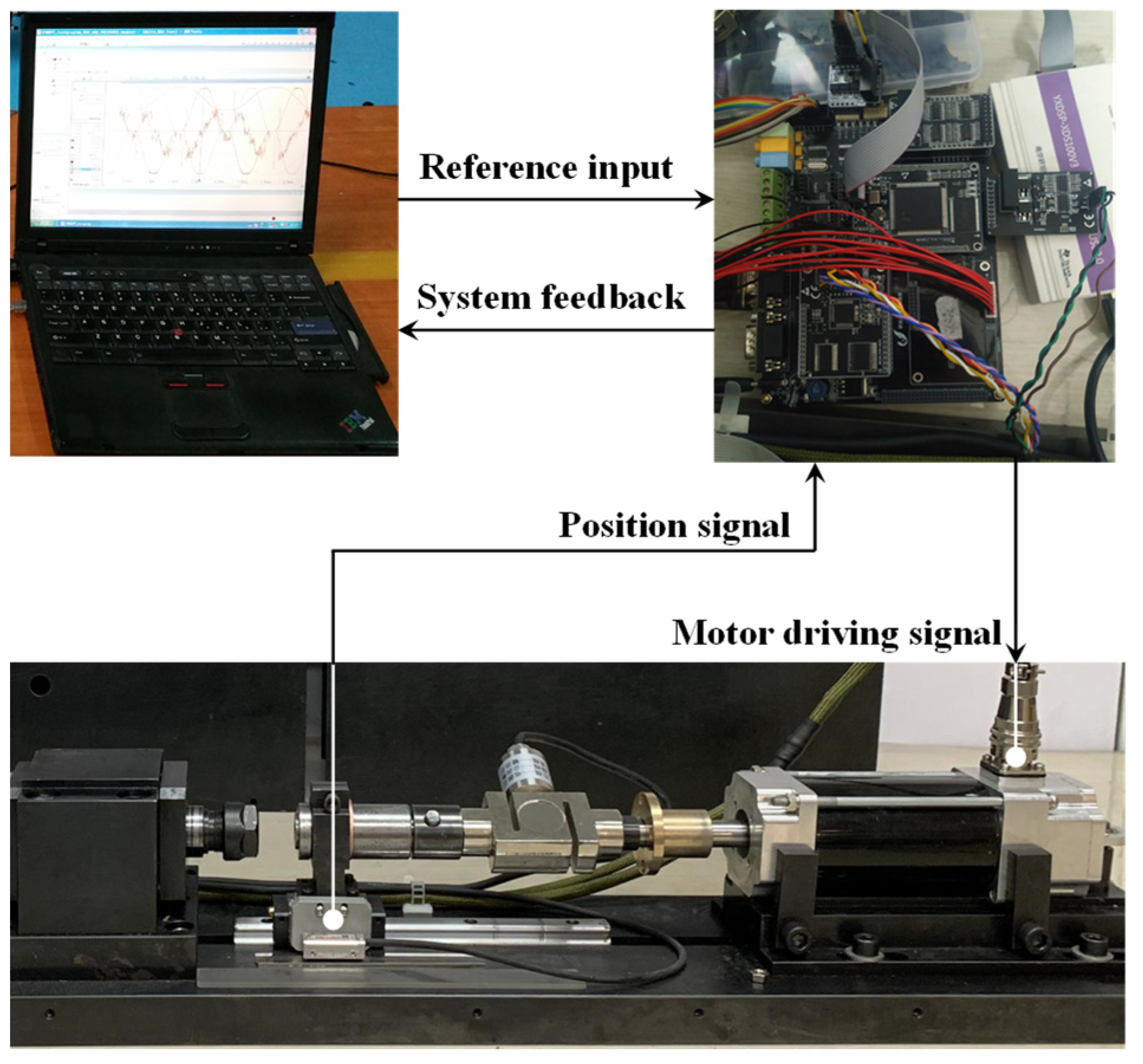
Figure 4.
Photograph of Test Rig.
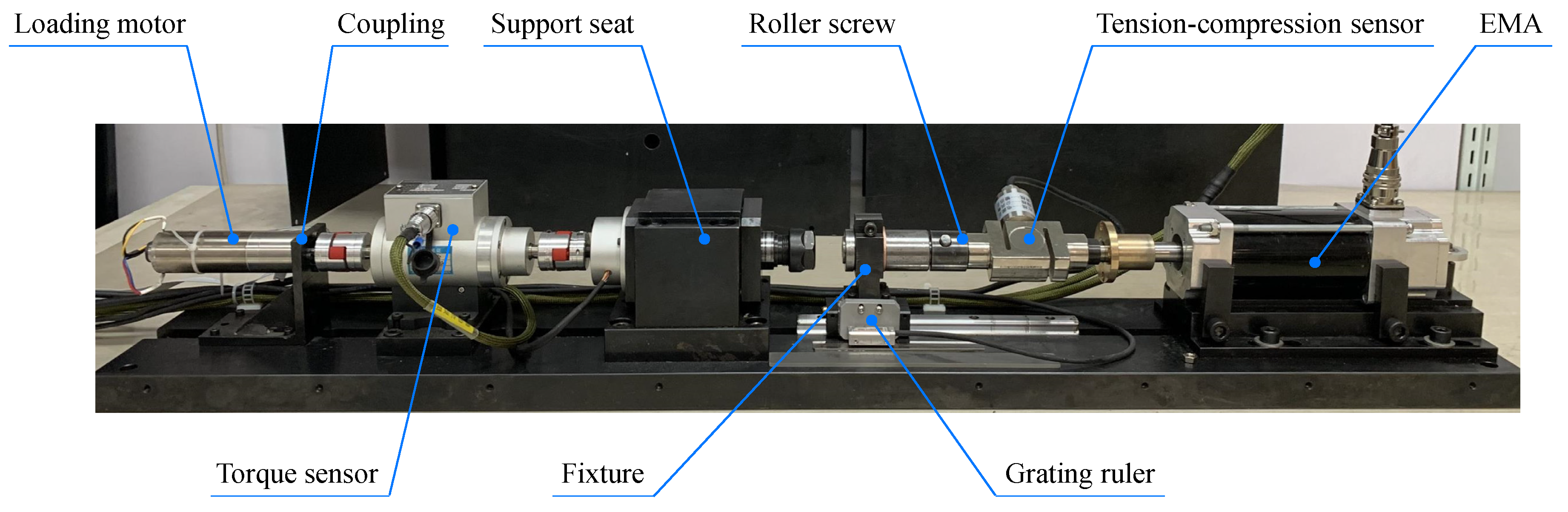
Figure 5.
PID Tracking Error of 0.2 Hz Sinusoidal Signal.

Figure 6.
ARC Tracking Error of 0.2 Hz Sinusoidal Signal.
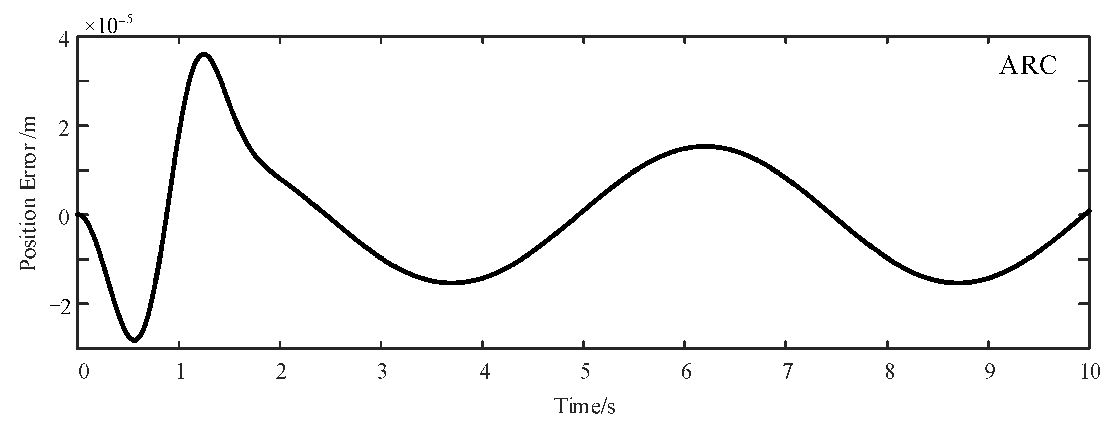
Figure 7.
ADRRAC Tracking Error of 0.2 Hz Sinusoidal Signal.
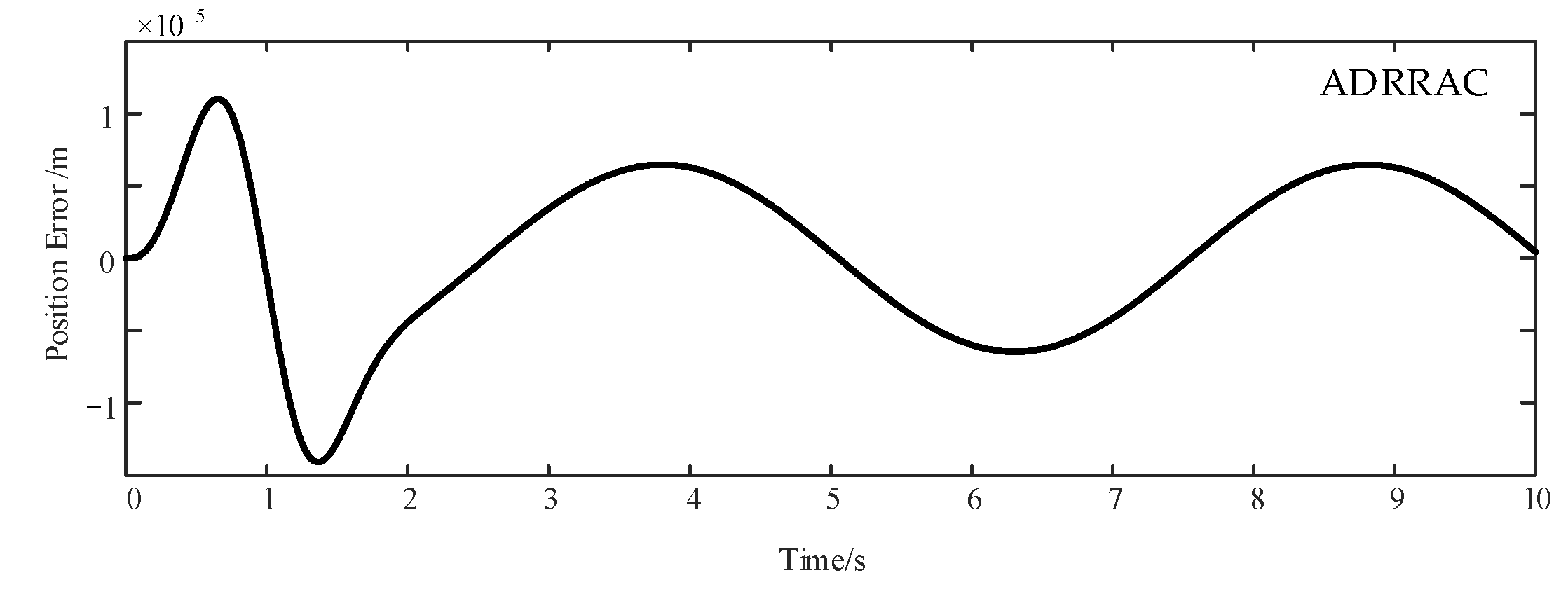
Figure 8.
PID Tracking Error of 1 Hz Sinusoidal Signal.
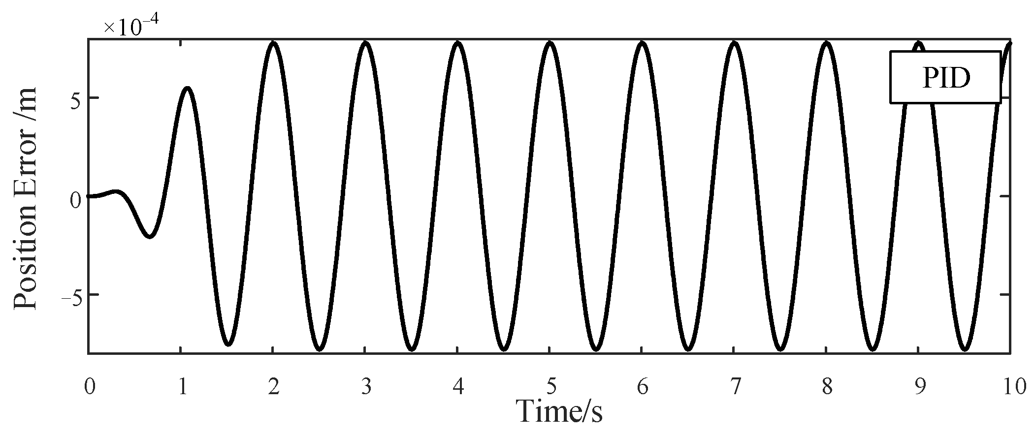
Figure 9.
ARC Tracking Error of 1 Hz Sinusoidal Signal.
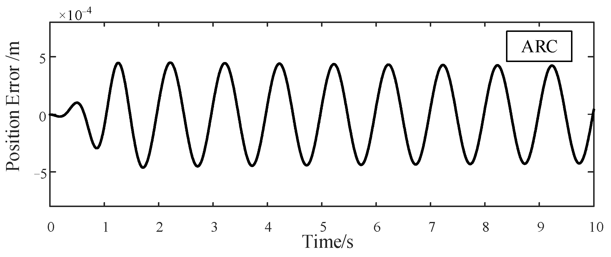
Figure 10.
ADRRAC Tracking Error of 1 Hz Sinusoidal Signal.

Figure 11.
PID Tracking Error of 1 Hz Sinusoidal Signal with 700 N External Disturbance.
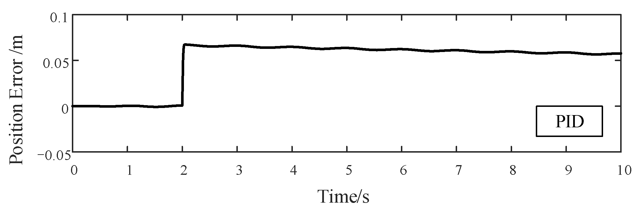
Figure 12.
ARC Tracking Error of 1 Hz Sinusoidal Signal with 700 N External Disturbance.
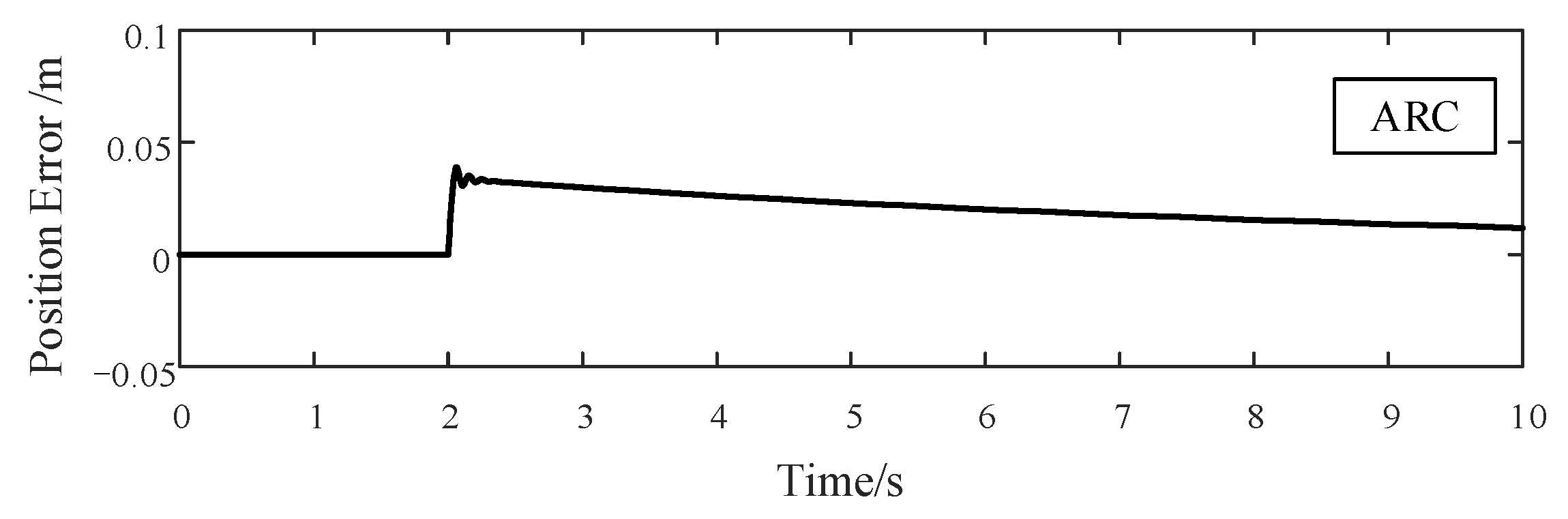
Figure 13.
ADRRAC Tracking Error of 1 Hz Sinusoidal Signal with 700 N External Disturbance.
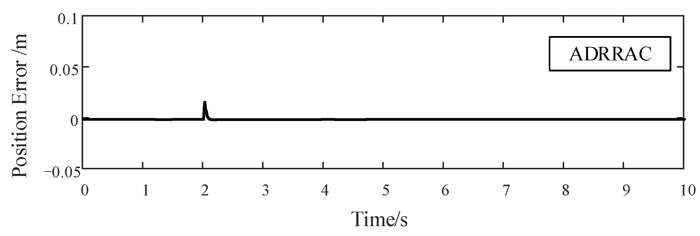
Figure 14.
Estimation of external disturbance of EDE.
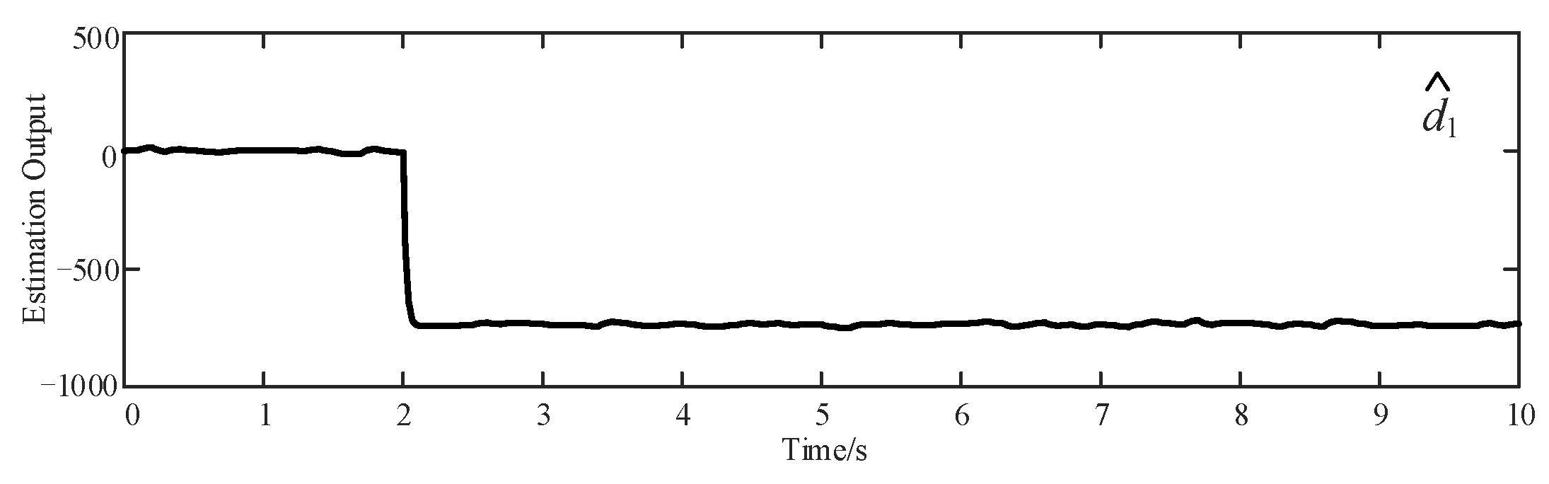
Figure 15.
Parameter Variation of ADRRAC Strategy.
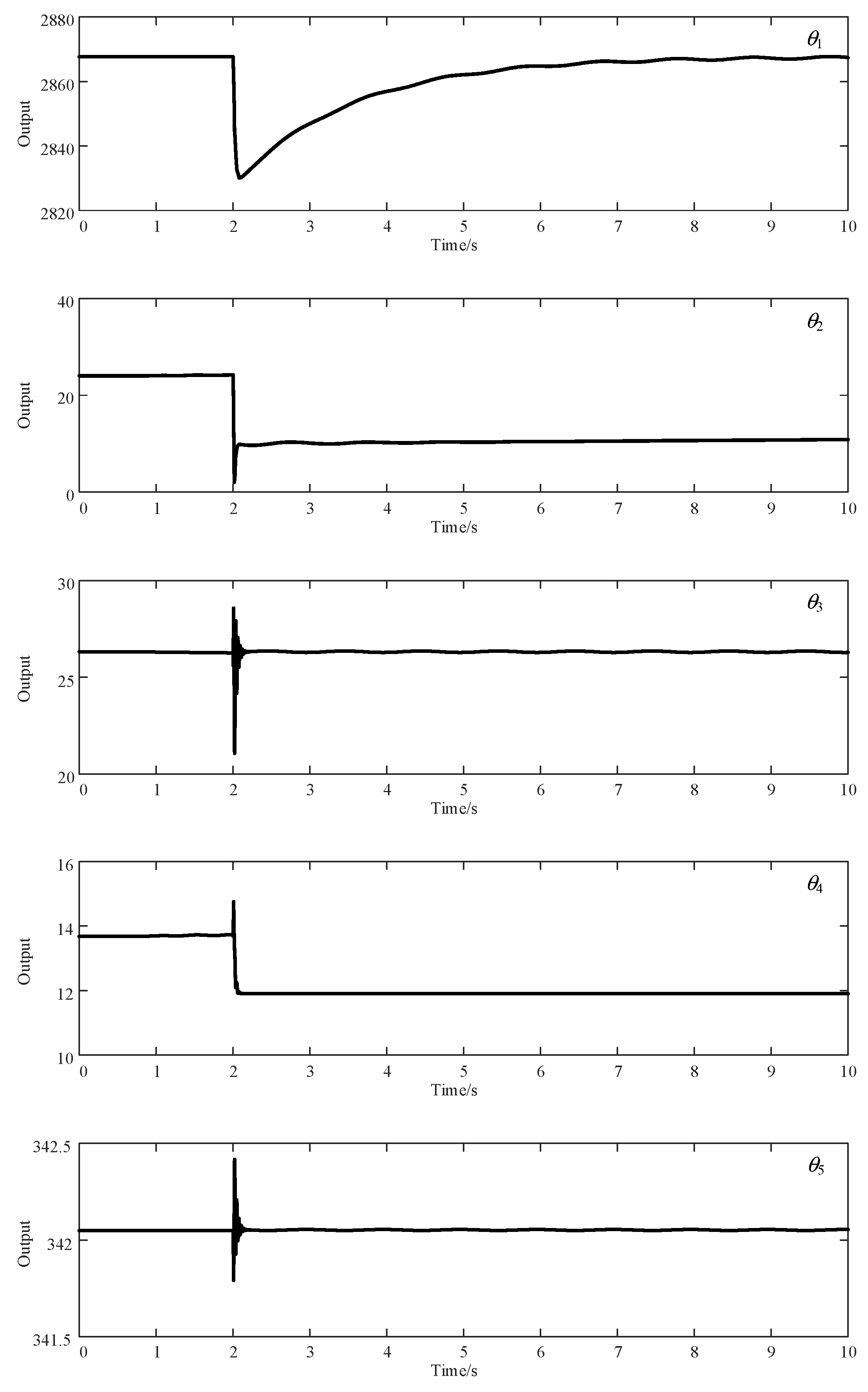
Figure 16.
Tracking Performance of 10 mm Step Signal.

Table 1.
Notations used for ADRRAC system.
| Symbol | Definition |
|---|---|
| Output displacement | |
| Output velocity | |
| Output accelerate | |
| Transmission efficiency | |
| External load | |
| Total inertia | |
| Viscosity coefficient | |
| Motor torque coefficient | |
| Screw transmission ratio | |
| System inductance | |
| System resistance | |
| Back EMF coefficient |
Table 2.
Performance indicators of 1 Hz sinusoidal inputs.
| Without Load | PID | ARC | ADRRAC |
|---|---|---|---|
| Average error | |||
| Peak error | |||
| Standard deviation | |||
| With Load | PID | ARC | ADRRAC |
| Average error | |||
| Peak error | |||
| Standard deviation |
Publisher’s Note: MDPI stays neutral with regard to jurisdictional claims in published maps and institutional affiliations. |
© 2021 by the authors. Licensee MDPI, Basel, Switzerland. This article is an open access article distributed under the terms and conditions of the Creative Commons Attribution (CC BY) license (https://creativecommons.org/licenses/by/4.0/).
Share and Cite
MDPI and ACS Style
Chen, Q.; Chen, H.; Zhu, D.; Li, L. Design and Analysis of an Active Disturbance Rejection Robust Adaptive Control System for Electromechanical Actuator. Actuators 2021, 10, 307. https://doi.org/10.3390/act10120307
AMA Style
Chen Q, Chen H, Zhu D, Li L. Design and Analysis of an Active Disturbance Rejection Robust Adaptive Control System for Electromechanical Actuator. Actuators. 2021; 10(12):307. https://doi.org/10.3390/act10120307
Chicago/Turabian StyleChen, Qinan, Hui Chen, Deming Zhu, and Linjie Li. 2021. "Design and Analysis of an Active Disturbance Rejection Robust Adaptive Control System for Electromechanical Actuator" Actuators 10, no. 12: 307. https://doi.org/10.3390/act10120307
Note that from the first issue of 2016, this journal uses article numbers instead of page numbers. See further details here.