Abstract
Convolutional Neural Networks (CNNs) and Deep Learning (DL) revolutionized numerous research fields including robotics, natural language processing, self-driving cars, healthcare, and others. However, DL is still relatively under-researched in physics and engineering. Recent works on DL-assisted analysis showed enormous potential of CNN applications in electrical engineering. This paper explores the possibility of developing an end-to-end DL analysis method to match or even surpass conventional analysis techniques such as finite element analysis (FEA) based on the ability of CNNs to predict the performance characteristics of electric machines. The required depth in CNN architecture is studied by comparing a simplistic CNN with three ResNet architectures. Studied CNNs show over 90% accuracy for an analysis conducted under a minute, whereas a FEA of comparable accuracy required 200 h. It is also shown that training CNNs to predict multidimensional outputs can improve CNN performance. Multidimensional output prediction with data-driven methods is further discussed in context of multiphysics analysis showing potential for developing analysis methods that might surpass FEA capabilities.
1. Introduction
Convolutional Neural Networks (CNNs) and Deep Learning (DL) have revolutionized various research fields becoming indispensable for computer vision, natural language processing, healthcare, robotics, and others real-life applications [1,2,3]. However, future saturation in conventional research areas is expected along with the growth of DL applications in areas where DL is currently underrepresented, including physics and various engineering fields [4,5,6,7]. Recent engineering applications include fault detection and material characterization along with DL-assisted analysis techniques [8,9,10].
DL methods allow making predictions for complex systems with various non-explicitly connected parameters, making them also promising for high-accuracy, fast, low-cost electromagnetic analysis. The latter is extremely important for the design of high-density high-efficiency electric machines that have various industrial applications. Interior permanent magnet synchronous motors (IPMSMs) are highly valued for high power density, torque density, and energy efficiency owing to the properties of strong rare earth permanent magnets (PMs) [11,12]. They are widely used as traction motors for transport vehicles and in-wheel motors for electric vehicles [13]. Due to low-weight and compact size, IPMS motors and generators have been gaining increasing attention for more electric aircraft applications where compact lightweight high-torque machines are needed [14,15].
However, the design of IPMSMs involves geometry optimization for various output parameters including average torque maximization, torque ripple minimization, harmonic quality of back electromotive force (emf), and others. Furthermore, there are other important parameters such as overall efficiency, thermal stability, economic and environmental effects, and other parameters that are hard to account for using conventional design techniques [16]. Thus, for DL to be applied to electric motor design, an ability of a DL analysis tool to accurately predict multidimensional outputs must be investigated [17].
Nowadays, finite element analysis (FEA) is the most widely applied method for the analysis and design of electric machines due to its high accuracy. This method is also remarkably versatile, being applied to electrical, mechanical, fluid dynamics, and other analysis types. FEA uses numerical methods to find an approximate solution to field problems guided by, for instance, Maxwell equations in electromagnetism that have no analytical solution. However, the high accuracy comes at a price of enormous computational time resulting in high computational costs.
Whereas FEA finds the solution by minimizing errors over numerous iterations, the computation results are eventually dismissed and never used for future analyses. Therefore, solving a problem for which a solution is known requires as much time as solving it for the first time. However, if there existed a method that could take advantage of previous computations to speed up future analyses, the prior data could be used to develop a high-accuracy high-speed analysis tool.
DL can facilitate such tools because after a time-consuming training stage, the prediction stage can be performed extremely fast. DL previously was applied to predict the distribution of arterial stresses as mechanical FEA surrogate model [18]. This work is computationally similar to electromagnetic field distribution prediction with DL [19]. In both cases, comprehensive information about the mechanical stress distribution or electromagnetic fields can be obtained. However, field distribution analysis approaches are hardware-demanding due to extremely large size of input and output data vectors and high complexity of DL models.
Recently, DL methods were applied to assist the optimization of high performance electric motors for traction and in-wheel motors. A custom CNN named multi-layer perceptron (MLP) was used to speed up the geometry parameter search for PMSM rotor geometry optimization for EV applications in [17]. Sasaki and Igarashi [20] used DL to assist the topology optimization using rotor RGB images as input data and optimizing for highest average torque. Similar work was done by Doi et al. [21] and Asanuma et al. [22] who also included torque ripple into DL predictor and achieved up to 30% faster optimization owing to the minimization of the number of FEA subroutine calls. Remarkably, the datasets used for DL training were about 5000 samples in size, showing the possibility of DL training on modest datasets for engineering analysis purposes, unlike extremely large million sample datasets commonly used in other research areas [23,24]. This is significant due to extremely high cost and time demands associated with dataset collection in engineering fields.
In the aforementioned papers, DL CNNs were primarily used to assist the analysis and the final results were still obtained using FEA. However, there is an enormous potential in developing end-to-end DL methods [9,25,26,27]. In this paper, DL CNNs are used for high-accuracy IPMSM output prediction. It is shown that training DL CNNs to predict multidimensional outputs, e.g., torque curves in case of this study, improves the analysis accuracy and allows for more comprehensive information about the IPMSM performance to be obtained.
Predicting torque curves rather than average torque or torque ripple is advantageous for electric machine performance analysis [28]. Several DL CNN architectures are studied to determine the required architecture complexity, including a simplistic custom architecture and ResNets of varying depth. A modest 4000 sample dataset collected using FEA is used for training, and the difficulties associated with collecting large datasets are discussed. Furthermore, different types of data normalization, dataset balancing, and potential errors associate with CNN training are also discussed. Finally, the high accuracy of CNN torque prediction is shown and the advantages over FEA are discussed along with future potential of DL CNNs to exceed FEA capabilities.
2. FEA Analysis of IPMSMs
2.1. IPMSM Rotor Geometries in JMAG Designer
In DL CNN training, typical IPMSM motor geometries were generated using JMAG Designer [29]. This tool provides an initial geometry shown in Figure 1, and several parameters that can be varied including stator and rotor diameters, numbers of poles and slots, slot size, permanent magnet (PM) size, and size of rotor slits.
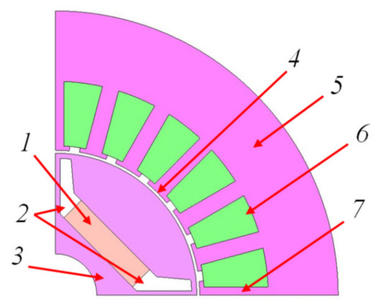
Figure 1.
Initial interior permanent magnet synchronous motors (IPMSM) geometry in JMAG Designer that includes the permanent magnet (PM) (1), rotor slits (2), rotor core (3), air gap (4), stator back iron (5), stator slots (6), and stator teeth (7).
This study focuses exclusively on rotor geometry, so stator parameters remain unchanged for all models. Furthermore, rotor outer diameter remains constant, leading to the position and size of the PM, and size and geometry of air slits being the variables. Table 1 summarizes the FEA parameters and parameter variation ranges for studied IPMSMs used to collect the training data. Stator current and PM grade remain unchanged for all experiments. The same approach can be used to obtain reluctance motor rotor geometries for DL studies [30]. Three-phase 60 Hz excitation is used in all models.

Table 1.
Finite element analysis (FEA) design parameters of studied IPMSMs.
As the purpose of electromagnetic analysis is to find the geometries that ensure high-performance of the motor, it might be tempting to exclusively use such geometries for DL model training. However, this might lead to DL developing bias towards predicting high-torque outputs, potentially predicting good results for geometries for which extremely low performance is realistically expected. To address this potential issue, an unbiased approached to data collection is utilized in this study, resulting in both optimal and suboptimal geometries shown in Figure 2 analyzed for DL training. This approach allows the features leading to both positive and negative results to be learned by the DL CNNs, thus accurately analyzing a large variety of low- and high-torque IPMSM rotor geometries.
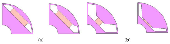
Figure 2.
Example IPMSM rotor geometries for (a) high torque positive and (b) extremely low torque negative examples.
For example, Figure 2a shows rotor designs with wide PMs positioned near the outer diameter of the rotor and slits focusing the PM flux into the air gap. These topologies produce high torque, and thus correspond to positive examples. On the contrary, Figure 2b shows small PMs positioned deep inside the rotor with unrealistically large slits. These topologies produce extremely low torque and are not realistically feasible. As mentioned above, such negative examples are included to teach the DL CNNs the features that lead to low torque, distinguishing them from the ones shown in Figure 2a.
2.2. FEA Model Parameters
FEA utilizes numerical methods, therefore its accuracy must be considered when preparing the training data. To ensure low computational errors and reasonable analysis time, a mesh study was conducted resulting in 6300 element (3700 nodes) mesh and analysis time of 2 s per step, 91 steps per geometry to obtain smooth torque curves.
The analysis time was approximately 3 min per model. Torque curves can be used to calculate the maximum torque, average torque, and torque ripple but provide additional essential information about harmonic spectrum of the torque and its distribution, which can be extremely valuable for IPMSM design.
It should be mentioned that unlike the models used in this study, an extremely high accuracy analysis may require hours for a single model to converge [31]. However, even 3 min per model still yields 200 h needed to analyze the 4000 sample dataset used in this study not including the FEA model setup time, loading time, exporting and interpreting the results, and other ancillary but necessary operations. This illustrates the difficulties associated with collecting large datasets for DL electrical engineering applications.
3. Preparing the Training Data
3.1. Arranging Rotor Images and Torque Curves for DL Training
DL CNNs take advantage of training on large datasets, and deep models are often characterized by an extremely large number of parameters and layers making their implementation computationally demanding. In this study, the experiments are conducted with smaller input image size to reduce the hardware requirements and training time while ensuring that the accuracy of input data representation is not compromised. Similar approaches to data preparation were previously implemented by other researchers [22,30].
With JMAG Designer it is possible to export rotor geometries as RGB images with default resolution of approximately 180 × 180 pixels. However, this resolution was found suboptimal due to large size and no information carried by color channels. Thus, the input images are resized to 56 × 56 pixel resolution and converted to grayscale as shown in Figure 3. The resolution was also chosen to be a divisible of the default input of ResNets to apply the latter without modifying the filters.
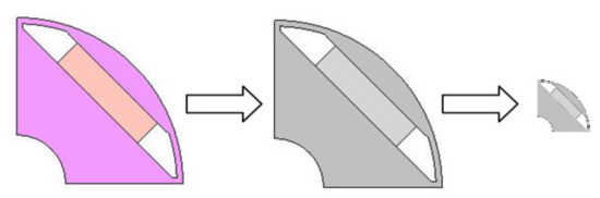
Figure 3.
Preparing rotor images for convolutional neural network (CNN) training by converting to grayscale and resizing JMAG Designer exported rotor geometries.
Pytorch 1.4.0 is used in this study for DL CNN implementation, training, and data preparation [32]. The grayscale rotor geometry images are first converted to numpy arrays and paired with corresponding output torque data [33]. Data normalization and torque clipping discussed in the next subsection are also performed on this stage. The dataset is later converted to Pytorch tensors for DL model training. Numpy arrays and Pytorch tensors with the dataset prepared for training can be exported and saved for later use by various CNN models.
It should be stressed that a simplistic geometry presented in Section 2.1 is chosen because the main purpose of this paper is to explore the possibility of predicting multidimensional outputs with CNNs. When a successful method is developed it could be applied to more complex geometries that might include flux barriers, Halbach array magnets, and other novel flux-focusing techniques [34,35]. When figures are used as input data, all relevant features are extracted by the DL model. This would not be the case when a vector of predefined design parameters is used. Whereas the latter could lead to smaller size of data vectors and potentially faster training, generalization of such method would be impossible as adding new parameters would require retraining the DL model. On the contrary, using figures does not define the parameters explicitly allowing for better generalization.
3.2. Min-Max and Offset Torque Normalization Techniques
In electric machines, the output torque range can be extremely large, especially for diverse datasets with negative examples contributing to very low torque values as well as near-optimal geometries with high torques. This is drastically different from DL classification where binary 0 or 1 outputs have to be predicted.
Predicting the exact numerical output values for electric machines is a regression problem. Whereas it is in principle possible to predict any numerical value with CNNs, they perform better when an arbitrary range of outputs is normalized using, for instance, min-max normalization [36]:
where is normalized torque, and and are minimum and maximum torque values in the dataset, respectively. This leads to being within the 0–1 range.
In case of torque calculation, the exact numerical values in output layers of CNN are compared with dataset torques. It was noticed that predicting a large data range with high precision was challenging, as shown in Section 5. This might be due to disproportional contribution of smaller values to relative error metric.
However, accurately predicting extremely small torque values is not important because they are associated with negative examples. Furthermore, it is desired to predict large outputs of optimal geometries with the highest possible accuracy. Thus, the use of a different normalization that reduces the effect of low torque samples on DL training can be proposed. An offset in normalization range can be introduced so that
where is normalization offset parameter so that . Using (2) essentially leads to all torques being treated in exactly the same manner, hence removing the strain of predicting their exact values accurately. The normalized outputs predicted by DL CNN can be then recalculated into the real ones as
It was observed that training DL CNNs on the data normalized using (2) led to higher prediction accuracy and faster convergence. It should be mentioned that using (2) results in additional errors for values close to when calculating real values using (3). Therefore, should be chosen so errors are large only in regions where high accuracy is not required. Choosing a small does not result in error increase for average and large torque samples.
Alternatively, the dataset can be clipped for low torques so that
where is a threshold parameter. The effect of is similar to the effect of , so accuracy at extremely low torques is disregarded to ease the training for the rest of data range. However, no additional error is introduced for unlike in case of offset normalization, making torque clipping a better option.
It should be noted that losing accuracy at low torques is acceptable in this study because associated geometries are flawed and correspond to negative examples. However, applying (2) may result in poor accuracy when only positive examples are used to train the model, or the complete torque range needs to be predicted with the same accuracy.
3.3. Data Balancing for Training and Testing
DL CNNs can potentially overfit the training data leading to the model performing well on the training set, but failing on any example outside the initial dataset. Thus, the complete dataset is divided into training, validation, and test sets. The majority of available data is usually allocated for training. In this study, 80% of the dataset is training data. In case the training data is limited, the validation and training sets can be merged, which applies to 4000 sample dataset used in this study. Thus, 20% of dataset is allocated for validation and validation accuracy is used to calculate the accuracy metrics.
Before dividing into training and validation, the dataset is shuffled to avoid clustering of similar examples. Both training and validation sets are checked for balance, meaning that all types of data (low, average, and high torque samples) are equally represented to ensure unbiased training and validation.
4. DL CNN Architectures and Training Parameters
Electric machine researchers previously used very deep architectures such as GoogLeNet [21,37], and even VGG 16 that has 138 m parameters [22,38]. However, smaller custom architectures were also used successfully [30]. Thus, it is currently hard to determine the optimal CNN architecture required for electric machine design projects.
To address this problem, a custom simplistic low-demand CNN is compared with different ResNet architectures. The torque prediction accuracies are compared along with size, complexity, and hardware requirements of the architectures.
4.1. Custom Simplistic Architecture
In this study, a simplistic CNN shown in Figure 4 is used to evaluate the possibility of training shallow networks for electric machine design projects. Table 2 shows that this CNN consists of three convolutional and two fully connected (linear) layers and has less than 1 million parameters. The ratio of the number of channels in convolutional and linear layers mimics the intermediate layers of AlexNet [39]. This architecture was inspired by the success of shallow networks on image classification tasks.
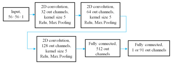
Figure 4.
Architecture of the 5 layer Simplistic CNN with less than 1 million parameters.
Table 2.
Comparison of parameters of studied DL CNN architectures.
The advantage of using shallow CNNs is fast training and low memory demands. A small size of this architecture allows training to be performed reasonably fast even on CPU, unlike deeper architectures for which CPU training takes unreasonably long and GPU training is strongly recommended.
4.2. ResNets
ResNets [40] are deep residual CNNs that were developed to explore the relation between the depth and image classification accuracy inspired by the evidence of accuracy degradation for extremely deep architectures [41]. ResNets introduced bypass connections and trained network to learn desired change of activations instead of activations themselves. The architectures consist of blocks of convolutional layers with block types and their number specifying particular architectures. All ResNets have one initial convolutional layer and one linear output layer, with aforementioned blocks of convolutional layers allocated between them. The softmax operation on the output layer used by classifiers is removed for regression problems.
ResNet-50 and more complex architectures utilize four bottleneck-type blocks with two identity mappings surrounding a 3 × 3 convolution. The ResNet-50 parameters can be encoded as [3, 4, 6, 3] with each number corresponding to the number of blocks of each type. Table 2 shows that ResNet-50 has 50 layers, of which 49 are convolutional. This is the deepest architecture among the architectures studied in this paper with almost 24 million parameters.
Less deep ResNet architectures use basic blocks with two 3 × 3 convolutions per block. Table 2 shows that ResNet-18 utilizes two blocks of each type and has roughly half the ResNet-50 parameters. In addition, an even shallower architecture is considered with only one block per type, resulting in the total of 10 layers, labeled ResNet-10.
4.3. DL CNN Training Parameters
CNN training, as training of any artificial neural network, is an optimization process where errors calculated during forward pass are backpropagated to update the network weights and minimize errors. Adam optimizer is used for all experiments in this study [42].
There are several important hyperparameters that affect the training. First, learning rate determines the step size in optimization process. On one hand, large learning rate facilitates faster training but may result in oscillations and divergence leading to unstable training. On the other hand, small learning rate may lead to very slow training or solutions stuck at saddle points. Thus, it is often recommended to monitor variation in training and validation losses and update the learning rate, respectively. This can be done manually or automated using learning rate decay [43].
For most experiments on ResNets, a common 0.01 initial learning rate and 0.1 learning rate multiplier were found effective. However, for the Simplistic CNN, the latter settings often resulted in poor convergence. A 0.5 initial learning rate and 0.2 learning rate multiplier were empirically found to perform better.
Second, a loss function is used for error computation and CNN parameter adjustment during training. For regression problems, least absolute deviation (L1) and least square error (L2) loss functions are primarily used. In this study, nearly no difference was observed after comparing the two loss functions. However, L2 loss can be recommended because errors for high torques gain more weight compared to L1 loss, which is desired for accurate prediction in high-torque region.
Training CNNs can be very computationally expensive and requires high-end hardware. However, recent improvements in GPU training allowed fast training on affordable machines, or on GPU clusters for extremely large datasets. This is particularly relevant for CUDA-accelerated GPUs [44]. In this study, a NVIDIA GeForce GTX 1660 Ti GPU and CUDA 11.0 were used for all experiment.
The GPU memory should still be carefully managed when working with large datasets. Thus, training data is passed to the CNN using mini-batches, and mini-batch size is the third important hyperparameter. In Pytorch, a dataloader can also be used to automate the dataset splitting. In this study, a mini-batch size of 64 was used for all experiments. Whereas more shallow architectures allow mini-batch size to be increased, it was kept constant for clarity of comparison. To ensure that relatively small batch size did not result in added errors for shallow architectures, experiments on the Simplistic CNN were also conducted using batch sizes up to 256 which showed no significant deviation.
All CNNs were trained over 100 ÷ 180 epochs monitoring both training and validation losses with the termination point determined by the decay in the learning rate. As might be expected, training deeper CNNs took longer, with ResNet-50 training taking almost 6 times longer than the training of the Simplistic CNN.
4.4. Accuracy Metrics for Regression Models
Because training and validation losses are hard to interpret, the accuracy is calculated for final result interpretation using specific accuracy metrics. For classification problems, the percentage of correct predictions is the most commonly used accuracy metric. However, this is different for regression problems where purpose-driven metrics are needed. Whereas a single comprehensive accuracy metric for electric machine design problems is hard to propose, analyzing multiple metrics simultaneously can provide vital information about DL CNN performance.
First, mean average percentage error (MAPE) can be used [30,45] so that
where n is dataset size, and and are expected and predicted torque values, respectively. The accuracy is calculated using (5) as
Second, the accuracy of predicting the results within an error margin can be calculated as
where
and is error margin.
The gives a more general overview and is often used to analyse the accuracy of conventional modeling techniques. However, for a large dataset it can give misleading results when errors are localized in a particular part of the dataset.
5. DL CNN Torque Prediction Results
5.1. Comparison of Accuracy of Average Torque and Torque Curve Prediction by Different CNNs
In order to determine how dimensions of the output affect the CNN training, the Simplistic CNN along with ResNet-10 and ResNet-50 were trained to predict torque curves and average torques. For the latter experiment, the dimension of output layer was reduced from 91 to 1. The effects of the min-max and offset normalization were also studied by training the CNNs on differently normalized datasets.
The analysis results are summarized in Table 3 with accuracy calculated using (6). The experiments conducted on conventional (min-max) normalized datasets are labeled “conv.” in Table 3. It should be noted that the offset normalization and torque clipping discussed in Section 3 had nearly identical effects on CNN training, so “cust.” results in Table 3 are relevant for both techniques.
Table 3.
A1 average torque and torque curve prediction accuracy using conventional and custom normalization.
Table 3 shows that all CNNs performed better when trained to predict torque curves rather than average torques which might be not an intuitive finding. This can be explained by the multidimensionality of torque curves that provides CNNs with more information to learn the features from. This aligns with multi-task learning approach where training on several similar tasks in some cases provides better performance than training for a single task [46,47,48], or a single torque as in case of this study. Thus, training CNNs to predict output curves, or any type of distributed parameters potentially including different parameters types, is easier compared to predicting average values.
Furthermore, all models performed better when offset normalization or torque clipping were used. This can be attributed to the reduction in the variations in output torque. On one hand, Table 3 shows that accuracy of min-max normalized data prediction was gradually increasing with CNN depth, and it might be expected that deeper architectures with more parameters could perform better on such datasets. However, the accuracy exhibits saturation for extremely deep networks [40]. Furthermore, deeper networks are associated with more computational demands, longer training and higher costs. Therefore, introducing a meaningful threshold in the torque range can reduce the analysis costs by making CNN training faster and less dependent on the architecture depth.
5.2. Accuracy of Torque Curve Prediction
The accuracy of different CNNs predicting torques curves is summarized in Table 4. Accuracy metrics are applied to the complete dataset, and also exclusively to the high-torque samples. The latter allows the CNN performance in the region of interest to be evaluated with higher precision.
Table 4.
Torque curve prediction accuracy by different DL models.
First, Table 4 shows that the Simplistic CNN could not provide sufficient prediction accuracy. Whereas its overall MAPE accuracy is over 60%, it performs extremely poorly in mid- and high-torque ranges, as illustrated by other metrics. Figure 5 shows all models performing similarly on a low-torque sample, implying that the Simplistic CNN could successfully identify negative examples by predicting low torques and distinguishing such geometries from average-torque ones. This can be illustrated by Figure 6. However, Figure 7 shows that sometimes the Simplistic CNN was giving completely incorrect predictions. On the other hand, Figure 8 shows reasonable accuracy similar to Figure 6. So, whereas some success in identifying positive and negative examples qualitatively is shown by this architecture, it cannot be recommended for a quantitative analysis.
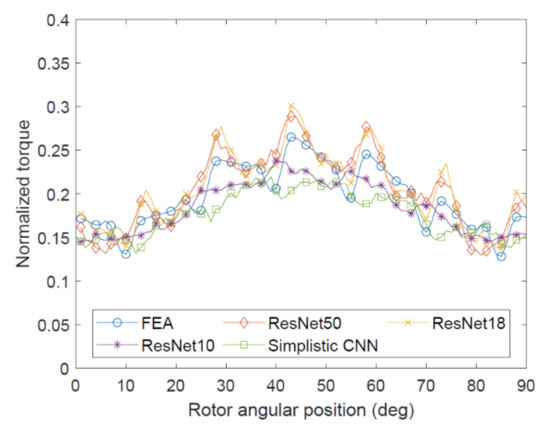
Figure 5.
Example of CNN outputs in low-torque region. All architectures show similar accuracy.
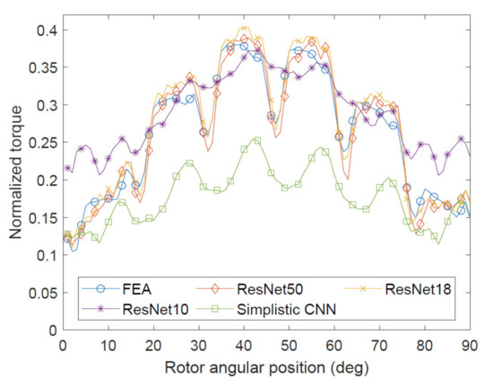
Figure 6.
Example of CNN outputs in low-mid torque region.
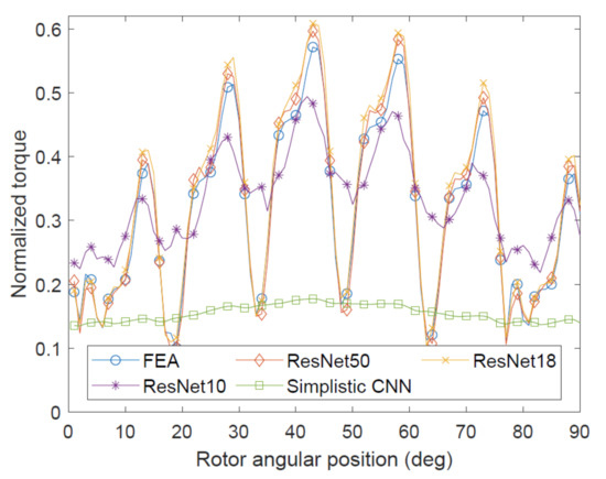
Figure 7.
Example of CNN outputs in mid-torque region.
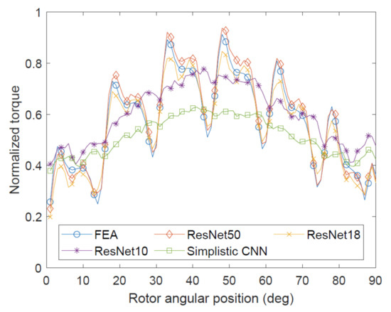
Figure 8.
Example of CNN outputs in high-torque region.
All ResNet architectures performed well on the dataset, showing MAPE accuracy of 88% or higher. However, some deviations illustrated by Figure 6, Figure 7 and Figure 8 were observed. It can be noticed that ResNet-10 tends to predict the torque magnitude reasonably well, but does not capture the shapes of the torque curves. This implies that the ResNet-10 parameters are not sufficient to capture all torque variations in the dataset, yet those are crucial for electric machine torque harmonic spectrum analysis. Low performance of ResNet-10 on error margin accuracy metrics also suggests that it tends to predict average values over groups of input samples, without further refinement into special features of particular geometries and their effects on the output torque.
On the contrary, ResNet-18 and ResNet-50 showed good agreement with FEA by capturing magnitudes and shapes of torque curves. As might be expected, ResNet-50 outperformed ResNet 18, but the latter still shows almost 90% accuracy on 20% error margin metric on the complete dataset, and about 80% accuracy on the 10% one.
It thus can be concluded that deep CNNs are capable of predicting output torque curves with high accuracy. The accuracy is proportional to CNN depth, and for sufficiently deep CNNs the number of CNN parameters correlates with the accuracy of curve shape prediction. However, this effect exhibits saturation as shown by the similar performance of ResNet-18 and ResNet-50.
5.3. Analysis Time of CNNs and FEA
Whereas ResNets show accuracy comparable to FEA, the analysis (torque prediction) time is significantly reduced when using CNNs, as shown by Table 5. Evaluating the complete dataset even with ResNet-50 takes less than 1 min, whereas FEA requires 200 h of computations. Furthermore, the FEA models used in this study were relatively compact, whereas extremely high-accuracy FEA may take up to 1 h per model or even longer, further escalating the difference between FEA and CNN prediction times. However, CNNs can be trained on the data obtained using high-accuracy FEA models, and then reused taking advantage of extremely fast CNN prediction speeds.
Table 5.
Analysis time of FEA and different CNN architectures.
Because of high speed of CNN analysis, IPMSM rotor geometry optimization can be performed extremely fast when FEA is substituted for a DL tool and optimization algorithms are applied. Whereas DL CNNs were previously used to speed up the optimization while final results were obtained using FEA [20,22], this paper shows the possibility of accurately evaluating rotor geometries using DL CNNs. Thus, the previously reported DL-accelerated optimization results can be further improved by developing a complete FEA-free end-to-end DL analysis method.
6. Discussion
6.1. Comparison of the Proposed End-to-End Method with Existing DL-Assisted Methods
DL-assisted design has gained popularity in recent years. As right now the field is rapidly progressing, it is worth comparing this paper’s results with the previously published ones. In some of previous works, namely, those in [20,21,22], DL classifiers were used instead of DL regression algorithms. However, using a classifier allows only a torque range to which a particular design correspond to rather than the exact torque values to be predicted, thus compromising the prediction accuracy. Using classifiers in those papers was possible because final results were still computed using FEA, and the role of DL was to reduce the number of steps in optimization algorithm rather than predicting final output values. In [20,21,22], the reduction in the analysis time was found to be 10–33% depending on a particular study. However, Table 5 shows that the analysis can be accelerated much more when DL-exclusive analysis methods are used and no additional calls to FEA are required. Furthermore, the works in [20,21,22] as well as in [30] focused on predicting only average torque and torque ripple values, so only two output parameters were predicted by CNNs. On the contrary, CNNs in this study predict torque curves constituted of 91 data points per curve. This result is also very important not only for torque curve prediction, but for multiparameter prediction in general, as discussed in detail in the next subsection.
Regarding CNN complexity, the works in [20,21,22] used extremely deep networks like VGG16. However, Section 4 and Section 5 show that more shallow networks are sufficient for analysis and design projects because prediction accuracy exhibits saturation. Using more shallow CNNs speeds up the analysis, as shown in Table 5. This result is also supported by the findings in [30] where an average depth custom CNN was found sufficient for high accuracy prediction that also sped up the analysis by almost 20 times.
It is interesting that the authors of [22] reported that the analysis accuracy improved when different rotor geometries, those with D- and V-shaped magnets, were included into the same training dataset. Therefore, the prediction accuracy of DL methods increases for datasets with various rotor geometries. It also increases with more output parameters, as shown in Section 5 of this paper. Therefore, DL methods are extremely promising when analyzing different machine types with a variety of output parameters.
It is important that the authors of [9,17,20,21,22,30] showed that DL methods can be seamlessly combined with optimization algorithms, implying that the method proposed in this paper would have such property, too. Indeed, full advantage of rapid output parameter prediction using CNNs will be taken when it is combined with optimization algorithms. Whereas optimizers are inherently fast, the requirement of conventional methods to make calls to FEA slows down the analysis due to high computational costs of the latter. Therefore, fast DL predictors combined with rapid optimization could be the key for extremely low computational cost analyses. However, predicting distribution of output parameters discussed in this paper is essential for developing comprehensive DL predictors. Ultimately, multiparameter predictors that can be easily combined with optimization algorithms are desired. The capability of the results presented in Section 5 to be extended to multiparameter analysis is discussed in the next subsection.
6.2. Potential Application of DL Tools to Multiparameter Multiphysics Analysis
Whereas up to this point CNN training to predict a single output type, namely, torque values and torque curves, was discussed, there are many more parameters of interest in machine design, including efficiency, reliability, potential overheating, mechanical loads, and others. For instance, efficiency map prediction with CNNs was reported in [9].
DL techniques inherently do not have restrictions on types of data they are trained to predict. In case of image recognition, every point in the output vector corresponds to a different class of objects being recognized requiring no correlation between the classes. For machine design, this implies that the output vector could include all meaningful information about the machine. As it was shown in Section 5 that multidimensional outputs could be predicted with high accuracy for machine performance evaluation projects, this indicates a possibility of conducting multiparameter multiphysics analyses potentially surpassing the capabilities of conventional analysis methods.
In case of FEA, the possibility of solving multiphysics problems is limited by the availability of mathematical correlations between parameters. On one hand, this limits the number of physical processes that could be analyzed in a single model. On the other hand, this also typically prevents combining quantitative parameters with the qualitative ones. This makes the topics of reliability and economic or ecological aspects hard to incorporate with conventional methodologies requiring techniques different from the ones dedicated to machine performance evaluation. However, with DL even the data types with no apparent correlation could be combined, assuming the required datasets are available.
For quantitative multiparameter multiphysics analysis, the above discussion can be illustrated by the following example. When output torque is calculated using FEA as discussed in Section 3, another important parameter that can be extracted is back emf V curve. In this case, V and would have different magnitudes, but the same time step between points in the output vector due to the correlation between rotor angular position and time.
However, when thermal analysis of IPMSM motor is considered, the time over which the results should be collected must be increased significantly because thermal processes take longer than the electromagnetic ones. Conducting the analysis over one electrical period is insufficient to show the temperature change. Therefore, adding thermal analysis to the previously discussed experiment would be suboptimal either from electromagnetic or thermal analysis perspective. A similar problem can be encountered in case of mechanical strength analysis where, for instance, a mechanical stress on the rotor is analyzed. For the discussed experiment the mechanical stress is independent of time and can be represented by a single value.
However, the abovementioned parameters can be conveniently combined into a single predictor vector η for CNN training as shown in Figure 9. In this case, the time, or other parameter over which the results are obtained, is represented by the position i in η. By normalizing every parameter in η independently, their values become unitless and restricted to the [0, 1] region. For the above experiment, η can be constructed from different physical parameters as
where , , and are normalized values of torque, back emf, temperature, and mechanical stress, respectively. It should be stressed that each of the above parameters is normalized independently relative to, for instance, min-max values in their own datasets using (1). and indicate the beginning of a new parameter in η. CNN is then trained to predict η, which in general might contain data other than mentioned in this example. Real parameter values can be calculated from the predicted ones using an operation g converting normalized values to real ones as
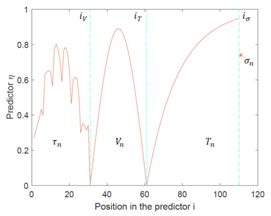
Figure 9.
Forming a single predictor vector η using normalized data corresponding to torque, back emf, temperature, and mechanical stress.
Function g would depend on normalization method for every parameter. Equation (3) is an example of .
It should be stressed that for CNNs the task of predicting η which encodes different types of data is computationally no different from predicting only the torque . When the data forming η is appropriately normalized (e.g., using Equation (9)), CNNs treat every point in η equally regardless of its physical meaning before normalization. This is an advantage of data-driven methods that allows the limitations related to mathematical formulations of couples analyses to be avoided. Thus, the fast high-accuracy prediction results in Section 5 could potentially be relevant for complex multiphysics analysis.
Similar methodology can be used to train CNN on datasets obtained by means other than FEA. The advantage of data-driven methods like DL methods is that accuracy does not depend on the type of data used for training. DL methods excel at finding correlation between input and output data regardless of its kind. Thus, when experimental datasets are used to train CNNs, the same >90% accuracy reported in this paper can be expected. Therefore, the method will perform well on experimental data, as it has been shown for other DL methods in the material study fields where experimental data is more readily available [25,26,27].
The main problem with training CNNs on experimental data is the current lack of suitable datasets. It was previously mentioned that in other research fields large datasets were collected and freely shared to facilitate the research. Therefore, the community effort is also required in engineering fields because collecting thousands to hundreds of thousands experimental and computational data samples is not feasible for a single research group. The success of DL multiphysics analysis tools strongly depends on the availability of suitable training data. Whereas it is possible to combine multiple data types into a single DL predictor, the initial data to train CNNs is still needed. Thus, collecting comprehensive datasets is essential for the successful development of generalized DL analysis tools in the future.
6.3. Current Limitations of DL Analysis Methods
However, there are several limitations that should be addressed for successful development of comprehensive DL design tools. First, in this paper, as well as in similar works on this topic, only the geometry serves as input data for CNN training. Table 1 shows that electrical current and material properties are constant, but different material combinations and operating regimes must also be considered for realistic design tasks. Thus, it is important to incorporate this information into the training data.
It can be recommended to use image channels to store this data. For conventional images the information in channels translates into colors. However, channels can be used to store any data, including additional machine or regime parameters. To avoid encountering associated increase in data loading time, data tensors with additional channels should be exported for future analyses as recommended in Section 3.1.
Second, a key to evaluating the real dimensions of the machine should also be stored in the channels when DL analysis is conducted on large datasets with different machine types, sizes, and power levels. As training is done on figures, there is a possibility that geometries that could be converted one into another via scaling become indistinguishable. Having an estimate of real machine size would allow this issue to be avoided.
Third, DL methods provide statistical accuracy. Section 5 shows that whereas the average prediction accuracy is high, the accuracy distribution could vary significantly throughout the dataset. Therefore, it is important to understand the degree of confidence towards particular predictions. It was recently proposed to provide an uncertainty measure in the CNN outputs providing a quantitative estimate of possible prediction errors [9].
Finally, as DL methods are data-driven, they would inherit errors associated with the training data collection method. In case of training on FEA data, this translates to inheriting computational errors inevitably associated with numerical methods. One potential solution is using extremely high-accuracy FEA to obtain high quality training data. Alternatively, training can be done on data obtained by other means, for instance, experimentally. However, conducting thousands of experiments on different machines is extremely expensive and time-consuming. Nevertheless, it should be considered that with the emersion of novel analysis methods new data acquisition techniques might provide the key to solving currently unresolved problems.
7. Conclusions
This paper investigates the possibility of predicting multidimensional outputs of electric machines with a DL CNNs. Four DL CNNs were trained to predict output torque curves of IPMSM showing over 90% prediction accuracy. It was shown that training CNNs to predict curves rather than single values (e.g., average torque and torque ripple) improves the prediction accuracy by providing more data for a CNN to extract the features from. The comparison of DL architectures investigates the required CNN depth for accurate torque prediction showing saturation for extremely deep CNNs. A custom normalization technique and an approach to dataset balancing are proposed showing positive effects on CNN training and torque prediction accuracy. In addition to high prediction accuracy, CNNs were evaluating torque curves 10,000 times faster compared to FEA.
The full advantage of the proposed method can be taken when it is combined with optimization algorithms. Furthermore, whereas the method is developed for IPMSM motors, it can also be used for other types of electric machines and other electromagnetic actuators. High-accuracy fast low-cost electromagnetic analysis is extremely important for the design of high-density high-efficiency electric machines that have various industrial applications. These include traction motors for transport vehicles, in-wheel motors for EV, low-weight compact high power density motors and generators used in more electric aircraft and ships. The method can also be applied to other types of electromagnetic actuators, such as stepping motors used in robotics, and high-precision linear actuators used in biomedical applications, assuming that relevant training data is used for CNN training.
Currently a great problem associated with the development of a comprehensive DL design tools is the lack of datasets for training. In other fields, where DL methods are already well-established, the research community efforts were undertaken to collect large datasets using which state-of-art DL CNNs were developed and tested. Thus, researchers in engineering fields are also encouraged to share their data so the same becomes possible for engineering design tasks. This paper shows that DL analysis tools are naturally capable of multiparameter multiphysics analysis and can include parameters that have no explicit mathematical correlation having potential to become major next generation analysis method for electric machines and other engineering applications.
Author Contributions
Conceptualization, N.G.; methodology, N.G. and A.V.; data acquisition, N.G. and S.M.; software, N.G. and S.M.; validation, N.G. and A.V.; formal analysis, N.G.; investigation, N.G.; writing—original draft preparation, N.G.; writing—review and editing, N.G., S.M. and A.V.; visualization, N.G. All authors have read and agreed to the published version of the manuscript.
Funding
This research received no external funding.
Institutional Review Board Statement
Not applicable.
Informed Consent Statement
Not applicable.
Data Availability Statement
The data presented in this study are openly available in Mendeley Data, doi:10.17632/j7bbrmmn4k.1.
Conflicts of Interest
The authors declare no conflict of interest.
References
- Lin, H.I. Learning on robot skills: Motion adjustment and smooth concatenation of motion blocks. Eng. Appl. Artif. Intell. 2020, 91, 103619. [Google Scholar] [CrossRef]
- Fink, O.; Wang, Q.; Svensén, M.; Dersin, P.; Lee, W.-J.; Ducoffe, M. Potential, challenges and future directions for deep learning in prognostics and health management applications. Eng. Appl. Artif. Intell. 2020, 92, 103678. [Google Scholar] [CrossRef]
- Bousquet-Jette, C.; Achiche, S.; Beaini, D.; Law-Kam Cio, Y.S.; Leblond-Ménard, C.; Raison, M. Fast scene analysis using vision and artificial intelligence for object prehension by an assistive robot. Eng. Appl. Artif. Intell. 2017, 63, 33–44. [Google Scholar] [CrossRef]
- Mehta, P.; Bukov, M.; Wang, C.H.; Day, A.G.R.; Richardson, C.; Fisher, C.K.; Schwab, D.J. A high-bias, low-variance introduction to Machine Learning for physicists. Phys. Rep. 2019, 810, 1–124. [Google Scholar] [CrossRef]
- Yin, J.; Zhao, W. Fault diagnosis network design for vehicle on-board equipments of high-speed railway: A deep learning approach. Eng. Appl. Artif. Intell. 2016, 56, 250–259. [Google Scholar] [CrossRef]
- Dong, Y. Implementing Deep Learning for comprehensive aircraft icing and actuator/sensor fault detection/identification. Eng. Appl. Artif. Intell. 2019, 83, 28–44. [Google Scholar] [CrossRef]
- Chen, H.; Jiang, B.; Zhang, T.; Lu, N. Data-driven and deep learning-based detection and diagnosis of incipient faults with application to electrical traction systems. Neurocomputing 2020, 396, 429–437. [Google Scholar] [CrossRef]
- Carpenter, H.J.; Gholipour, A.; Ghayesh, M.H.; Zander, A.C.; Psaltis, P.J. A review on the biomechanics of coronary arteries. Int. J. Eng. Sci. 2020, 147, 103201. [Google Scholar] [CrossRef]
- Khan, A.; Mohammadi, M.H.; Ghorbanian, V.; Lowther, D. Efficiency map prediction of motor drives using Deep Learning. IEEE Trans. Magn. 2020, 56, 7511504. [Google Scholar] [CrossRef]
- Omari, M.A.; Almagableh, A.; Sevostianov, I.; Ashhab, M.S.; Yaseen, A.B. Modeling of the viscoelastic properties of thermoset vinyl ester nanocomposite using artificial neural network. Int. J. Eng. Sci. 2020, 150, 103242. [Google Scholar] [CrossRef]
- Soliman, H.M. Improve the performance characteristics of the IPMSM under the effect of the varying loads. IET Electr. Power Appl. 2019, 13, 1935–1945. [Google Scholar] [CrossRef]
- Strinić, T.; Silber, S.; Gruber, W. The flux-based sensorless field-oriented control of permanent magnet synchronous motors without integrational drift. Actuators 2018, 7, 35. [Google Scholar] [CrossRef]
- Xu, X.; Zhang, G.; Li, G.; Zhang, B. Performance analysis and temperature field study of IPMSM for electric vehicles based on winding transformation strategy. IET Electr. Power Appl. 2020, 14, 1186–1195. [Google Scholar] [CrossRef]
- Madonna, V.; Giangrande, P.; Galea, M. Electrical power generation in aircraft: Review, challenges, and opportunities. IEEE Trans. Transp. Electrif. 2018, 4, 646–659. [Google Scholar] [CrossRef]
- Circosta, S.; Galluzzi, R.; Bonfitto, A.; Castellanos, L.M.; Amati, N.; Tonoli, A. Modeling and validation of the radial force capability of bearingless hysteresis drives. Actuators 2018, 7, 69. [Google Scholar] [CrossRef]
- Ilka, R.; Alinejad-Beromi, Y.; Yaghobi, H. Techno-economic design optimisation of an interior permanent-magnet synchronous motor by the multi-objective approach. IET Electr. Power Appl. 2018, 12, 972–978. [Google Scholar] [CrossRef]
- You, Y.M. Multi-objective optimal design of permanent magnet synchronous motor for electric vehicle based on deep learning. Appl. Sci. 2020, 10, 482. [Google Scholar] [CrossRef]
- Liang, L.; Liu, M.; Martin, C.; Sun, W. A deep learning approach to estimate stress distribution: A fast and accurate surrogate of finite-element analysis. J. R. Soc. Interface 2018, 15, 20170844. [Google Scholar] [CrossRef]
- Khan, A.; Ghorbanian, V.; Lowther, D. Deep learning for magnetic field estimation. IEEE Trans. Magn. 2019, 55, 7202304. [Google Scholar] [CrossRef]
- Sasaki, H.; Igarashi, H. Topology optimization accelerated by deep learning. IEEE Trans. Magn. 2019, 55, 7401305. [Google Scholar] [CrossRef]
- Doi, S.; Sasaki, H.; Igarashi, H. Multi-objective topology optimization of rotating machines using deep learning. IEEE Trans. Magn. 2019, 55, 7202605. [Google Scholar] [CrossRef]
- Asanuma, J.; Doi, S.; Igarashi, H. Transfer Learning through Deep Learning: Application to Topology Optimization of Electric Motor. IEEE Trans. Magn. 2020, 56, 7512404. [Google Scholar] [CrossRef]
- Deng, J.; Dong, W.; Socher, R.; Li, L.-J.; Li, K.; Li, F-F. ImageNet: A large-scale hierarchical image database. In Proceedings of the 2009 IEEE Conference on Computer Vision and Pattern Recognition, Miami, FL, USA, 20–25 June 2009; pp. 248–255. [Google Scholar]
- Google Open Source, Open Images Dataset. Available online: https://opensource.google/projects/open-images-dataset (accessed on 22 May 2020).
- Kusne, A.G.; Gao, T.; Mehta, A.; Ke, L.; Nguyen, M.C.; Ho, K.M.; Antropov, V.; Wang, C.Z.; Kramer, M.J.; Long, C.; et al. On-the-fly machine-learning for high-throughput experiments: Search for rare-earth-free permanent magnets. Sci. Rep. 2014, 4, 6367. [Google Scholar] [CrossRef] [PubMed]
- Gusenbauer, M.; Oezelt, H.; Fischbacher, J.; Kovacs, A.; Zhao, P.; Woodcock, T.G.; Schrefl, T. Extracting Local Switching Fields in Permanent Magnets Using Machine Learning. 2019. Available online: http://arxiv.org/abs/1910.09279 (accessed on 6 July 2020).
- Exl, L.; Fischbacher, J.; Kovacs, A.; Özelt, H.; Gusenbauer, M.; Yokota, K.; Shoji, T.; Hrkac, G.; Schrefl, T. Magnetic microstructure machine learning analysis. J. Phys. Mater. 2018, 2, 014001. [Google Scholar] [CrossRef]
- Kwang, T.C.; Jamil, M.L.M.; Jidin, A. Torque improvement of PM motor with semi-cycle stator design using 2D-finite element analysis. Int. J. Electr. Comput. Eng. 2019, 9, 5060–5067. [Google Scholar] [CrossRef]
- JSOL Corporation, JMAG Designer. Available online: https://www.jmag-international.com/products/jmag-designer/ (accessed on 4 June 2020).
- Barmada, S.; Fontana, N.; Sani, L.; Thomopulos, D.; Tucci, M. Deep Learning and Reduced models for fast optimization in electromagnetics. IEEE Trans. Magn. 2020, 56, 7513604. [Google Scholar] [CrossRef]
- Gabdullin, N.; Ro, J.S. Novel Non-linear transient path energy method for the analytical analysis of the non-periodic and non-linear dynamics of electrical machines in the time domain. IEEE Access 2019, 7, 37833–37854. [Google Scholar] [CrossRef]
- PyTorch—An Open Source Machine Learning Framework. Available online: https://pytorch.org/ (accessed on 26 May 2020).
- Numpy—Open Source Numerical Computation Library. Available online: https://numpy.org/ (accessed on 28 May 2020).
- Sayed, E.; Yang, Y.; Bilgin, B.; Bakr, M.H.; Emadi, A. A comprehensive review of flux barriers in interior permanent magnet synchronous machines. IEEE Access 2019, 7, 149168–149181. [Google Scholar] [CrossRef]
- Zhang, X.; Zhang, C.; Yu, J.; Du, P.; Li, L. Analytical model of magnetic field of a permanent magnet synchronous motor with a trapezoidal halbach permanent magnet array. IEEE Trans. Magn. 2019, 55, 8105205. [Google Scholar] [CrossRef]
- Grus, J. Data Science from Scratch; O’Reilly: Sebastopol, CA, USA, 2015; ISBN 978-1-491-90142-7. [Google Scholar]
- Szegedy, C.; Liu, W.; Jia, Y.; Sermanet, P.; Reed, S.; Anguelov, D.; Erhan, D.; Vanhoucke, V.; Rabinovich, A. Going deeper with convolutions. In Proceedings of the IEEE Conference on Computer Vision and Pattern Recognition, Boston, MA, USA, 7–12 June 2015; pp. 1–9. [Google Scholar] [CrossRef]
- Simonyan, K.; Zisserman, A. Very deep convolutional networks for large-scale image recognition. arXiv 2014, arXiv:1409.1556. [Google Scholar]
- Krizhevsky, A.; Sutskever, I.; Hinton, G.E. ImageNet classification with Deep Convolutional Neural Networks. Adv. Neural Inf. Process. Syst. 2012, 25, 1097–1105. [Google Scholar] [CrossRef]
- He, K.; Zhang, X.; Ren, S.; Sun, J. Deep residual learning for image recognition. In Proceedings of the IEEE Conference on Computer Vision and Pattern Recognition, Las Vegas, NV, USA, 26 June–1 July 2016; pp. 770–778. [Google Scholar] [CrossRef]
- He, K.; Sun, J. Convolutional neural networks at constrained time cost. In Proceedings of the CVPR, Boston, MA, USA, 7–12 June 2015; pp. 5353–5360. [Google Scholar]
- Kingma, D.P.; Ba, J.L. Adam: A method for stochastic optimization. In Proceedings of the ICLR, San Diego, CA, USA, 7–9 May 2015; pp. 1–15. [Google Scholar]
- Duchi, J.C.; Hazan, E.; Singer, Y. Adaptive subgradient methods for online learning and stochastic optimization. J. Mach. Learn. Res. 2011, 12, 2121–2159. [Google Scholar]
- CUDA—A parallel Computing Platform. Available online: https://developer.nvidia.com/cuda-zone (accessed on 31 May 2020).
- Myttenaere, A. De; Golden, B.; Grand, B. Le; Rossi, F.; Myttenaere, A. De; Golden, B.; Grand, B. Le; Rossi, F. Mean Absolute percentage error for regression models. Neurocomputing 2016, 192, 38–48. [Google Scholar] [CrossRef]
- Ruder, S. An Overview of Multi-Task Learning in Deep Neural Networks. 2017. Available online: http://arxiv.org/abs/1706.05098.
- Tan, Z.; De, G.; Li, M.; Lin, H.; Yang, S.; Huang, L.; Tan, Q. Combined electricity-heat-cooling-gas load forecasting model for integrated energy system based on multi-task learning and least square support vector machine. J. Clean. Prod. 2020, 248, 119252. [Google Scholar] [CrossRef]
- Li, M.; Chen, D.; Liu, S.; Liu, F. Grain boundary detection and second phase segmentation based on multi-task learning and generative adversarial network. Measurement 2020, 162, 107857. [Google Scholar] [CrossRef]
Publisher’s Note: MDPI stays neutral with regard to jurisdictional claims in published maps and institutional affiliations. |
© 2021 by the authors. Licensee MDPI, Basel, Switzerland. This article is an open access article distributed under the terms and conditions of the Creative Commons Attribution (CC BY) license (http://creativecommons.org/licenses/by/4.0/).