
Analytical and Experimental Investigations of Novel Maglev Coupling Based on Opposed Halbach Array for a 2D Valve


College of Mechanical Engineering, Zhejiang University of Technology, Hangzhou 310023, China
*
Author to whom correspondence should be addressed.
Actuators 2021, 10(3), 61; https://doi.org/10.3390/act10030061
Submission received: 15 February 2021
/
Revised: 12 March 2021
/
Accepted: 16 March 2021
/
Published: 17 March 2021
(This article belongs to the Section High Torque/Power Density Actuators)
Abstract
:In this paper, a novel maglev coupling based on the opposed Halbach array is proposed as the interface between the linear electro-mechanical converter and 2D valve body. This non-contact maglev coupling possesses several advantages over existing mechanical couplings such as zero friction and wear, low vibration and noise, and no lubrication, which is expected to greatly improve the control accuracy and life cycle of the 2D valve. A detailed analytical model of maglev coupling is established based on the electro-magnetic theory. Firstly, the permanent magnets of the Halbach array is decomposed into several types of basic elements to obtain their individual analytical expressions, which are then re-superimposed into the whole coupling to obtain the analytical formula of torque–displacement characteristics. In order to obtain maximum output torque of maglev coupling, a parametric analysis was performed using an analytical model and optimal pitch angle and shifted distance was explored and found. To verify the correctness of the analytical modelling and parametric analysis results, the torque–displacement characteristics were also studied through both the FEM simulation and experimental approach. The results of analytical modelling, FEM simulation and experiment were in a good agreement, which shows that the maximum magnetic torque can reach about 0.579 N·m when the external armature displacement is 1 mm. The research work provides an important reference for the future application of maglev coupling in a 2D valve.
1. Introduction
The electro–hydraulic control system has been widely used in crucial industries such as aerospace, defense, ship, large-scale power plant, and material testing machines [1,2,3]. As key control components, electro–hydraulic servo and proportional valves play a decisive role for the performance of the whole system [4,5]. In order to further improve the power-to-weight ratio and thus obtain competitive advantages over electrical drive technology, the electro–hydraulic servo and proportional valves have striven for the capability of high pressure and large flow rate since its advent [6,7,8]. Since the magnetic force generated by the electro-mechanical converter (EMC) is not sufficient enough to directly conquer the influence of Bernoulli force and friction force brought by high pressure and large flow rate condition, these valves need to be designed as pilot operated configuration where an extra pilot stage is supplemented so that the magnetic force of EMC can be effectively amplified to a sufficient level to actuate the main spool [9,10]. The pilot operated servo valves can be divided into nozzle-flapper valves, jet-pipe valves and deflector-jet valve, all of which are actuated by the torque motor. These valves are primarily aiming at aviation industry and therefore feature very fast dynamic response and high control accuracy [11,12]. However, they still have some disadvantages [13,14,15]. The first issue was the leakage flow of the pilot stage which could cost a considerable proportion of the input power given the system is idle for long periods. The second issue is the torque motor assembly that include some precise mechanical and electrical parts, which sacrifice simplicity, set-up and manufacturing costs. After World War II, the demand for low-cost and robust electro–hydraulic control technology from the civil industry was growing strongly, and the proportional valve appeared accordingly where the low-cost proportional solenoid was used as a valve EMC [16,17]. Similarly, some proportional valves used a pilot control approach to obtain a large flow rate. With the integration of the servo valve and proportional valve, the so-called industry servo valve emerged, where the high-performance linear force motor was used to directly actuate the valve and a linear variable differential transformer (LVDT) sensor was introduced to form closed loop control for the valve spool position [18,19]. Compared to the proportional valve, it possesses better static and dynamic response, while its advantages in terms of cost, stability and simplicity over the traditional servo valve remains. In order to simplify valve structure and obtain fast dynamics response, some novel valve configurations adopt functional materials as actuator to replace electro-magnetic EMCs [20,21,22,23]. However, the performance of such actuators is heavily influenced by limited working stroke and nonlinear hysteresis, which is still a long way to go from real industrial application.
For traditional hydraulic valve, the spool motion could be either singly translational or rotational inside the sleeve or valve body. However, these two distinct motions can be utilized simultaneously to constitute a novel pilot operated valve, which could be denoted as two-dimensional valve (2D valve) [24,25]. Since the spool of the 2D valve physically functions as both the pilot stage and main stage, therefore, it features simplicity and high power-to-weight ratio [26,27]. Nevertheless, this configuration needs to design a spiral-shape sensing groove on the sleeve inner surface in order to regulate pressure in the control chamber. The manufacturing cost of such a groove is high since a special machining tool is usually needed. Moreover, the valve needs to be driven by a rotary electro-mechanical converter (REMC) to rotate spool firstly to actuate “2D” mechanism. However, the REMC has the disadvantages of a small market and therefore high cost because it is not so popular as linear electro-mechanical converter (LEMC) such as proportional solenoid [28]. Overall, this valve configuration is more appropriate for applications such as the aviation and military industry where performance occupies top priority and costs are less sensitive.
The civil servo industry usually prefers a low-cost product. In order to promote a 2D valve to the industrial hydraulic field, a special coupling was introduced between EMC and the valve body to realize the spool position feedback and motion conversion. The advantage of this configuration was that the original spiral sensing groove can be simplified as a simple, rectangular sensing groove and a commercial proportional solenoid can be available as an EMC, which could reduce both the costs of manufacturing and valve EMC. There were several types of such mechanical couplings proposed in the literature, such as the coupling of roller and sliding-wedge pair [29], the coupling of ball screw pair and coupling of leaf spring [30], as shown in Figure 3b. The main defect of these couplings lies that the friction and wear coming from the mechanical contact has obvious influence on the valve control accuracy. Moreover, the mechanical couplings usually require lubrication, and accompanying vibration and noise also affect the service life of the valve.
In order to eliminate the unfavorable influence from the friction and wear of mechanical coupling, novel maglev coupling based on the opposed Halbach array was proposed in this paper, which was used to suspend the internal armature-spool assembly in the middle position using magnetic repulsive force and realize the function of spool position feedback and motion conversion by a non-contact way. Compared to the existing mechanical couplings, this non-contact maglev coupling possesses several advantages such as zero friction and wear, low vibration and noise, and no lubrication, which is expected to greatly improve the control accuracy and life cycle of the 2D valve.
The rest of this paper is organized as follows: in Section 2, the configuration and working principle of maglev coupling is introduced. In Section 3, a detailed analytical model of maglev coupling is established based on the electro-magnetic theory. In Section 4, a parametric analysis is performed using analytical model and optimal pitch angle and shifted distance are searched and found. In Section 5, an FEM simulation is performed to validate analytical modelling and parametric analysis results. In Section 6, a prototype of maglev coupling is manufactured, and the torque–displacement characteristics are studied through experimental approaches. Finally, some conclusions of this work are drawn in Section 7.
2. Configuration and Working Principle
Figure 1 illustrates the configuration of maglev coupling, which mainly includes external armature, internal armature, permanent magnets (PMs), linear bearing, and guide pin. The pole surfaces of the external armature and internal armature are deliberately designed to be inclined with pitch angle , where these angles are all the same and arranged by a 180° array. One end of the guide pin is fixed with the valve body cover, and the other end is inserted into the linear bearing, thus the external armature is guided to move linearly only, while the internal armature can move both linearly and rotationally. The pole surfaces of the external armature and internal armature are all inserted with several PMs. In order to increase magnetic intensity in the air gap, an opposed Halbach array is adopted for the arrangement of these PMs. Figure 2 illustrates the detailed configuration and magnetization directions where at least three different PMs are used to constitute each part of Halbach array. Note that more PMs are also feasible, however, it would increase assembly difficulties. The magnetic forces generated by upper section and the lower section of Halbach array should be mutually repulsive so that the internal armature can be levitated in the middle of the external armature in a non-contact way.
Figure 3a shows a schematic for the configuration of a novel 2D valve based on maglev coupling. It is composed of linear electro-mechanical converter (LEMC), maglev coupling and a 2D valve body. The LEMC is connected with external armature, whose output force is transferred to the displacement of external armature via a compressed spring. The 2D valve body mainly consists of spool and valve sleeve. Two tiny rectangular holes called the hp-hole and lp-hole were manufactured on the right spool land and ported to oil supply and reservoir, respectively. There is a rectangular sensing groove machined on the inner surface of the sleeve, which is piloted to the control chamber on the right end of spool. The oil supply pressure is led to the hp-hole and high-pressure chamber through hole a and hole b. In the equilibrium position, the hp-hole and lp-hole were located on the two sides of rectangular groove and constitute two tiny overlapping openings, which forms a half-hydraulic resistance bridge. The output pressure of the resistance bridge is then ported to the control chamber. Neglecting Bernoulli’s force and friction force and set the area of the control chamber as twice as that of the high-pressure chamber, so the spool can be in a hydrostatic force balance.
Figure 4a,b illustrate the detailed force analysis for maglev coupling. The magnetic repulsive forces generated by the Halbach array, i.e., , , , can be further resolved into axial components , , , and tangential components , , , . When LEMC is not electrified, the magnetic repulsive forces are equal, as shown in Figure 4a, and the hp-hole has the same overlapping height with respect to the sensing groove as does the lp-hole. Therefore, the pressure of the control chamber regulated together by the hp-hole and lp-hole is , and the pressure area of the left high-pressure chamber is half of the right control chamber. Thus, the assembly of the internal armature-spool is under a state of static balance. When LEMC is electrified, the external armature moves , and the , , , decreases and the , , , increases, as shown in Figure 4b. Among them, the resulting force of axial components would be compensated by the Bernoulli force , and the resultant force of tangential components would generate a torque to drive the spool to rotate clockwise, as shown in Figure 4c, and this rotary motion changes two overlapping openings differentially, which varies the control chamber pressure and causes the imbalance of hydrostatic force acting on the spool, therefore the spool moves towards the right. This linear motion of the spool again results in the changes of magnetic repulsive forces, which leads to the reverse rotation of the spool until these forces return to their initial value, and the overlapping openings of hp-hole and lp-hole with sensing groove equals again. As a result, the force balance is re-established and the spool is in a new equilibrium position.
3. Analytical Modelling
3.1. Analytical Modelling of Permanent Magnet Units
Figure 5 demonstrate two infinitesimals of permanent magnet (denoted as IPM) with unit length in the y axis direction, where , are the area of IPM-1 and IPM-2, respectively; , are the residual magnetic induction intensity of IPM-1 and IPM-2, respectively; , is the angle between , and the positive direction of x axis; is the distance between IPM-1 and IPM-2 in the xoz plane; is the angle between and the positive direction of the x axis. According to the theory of point magnetic charge, if IPM-2 is placed in the magnetic field generated by IPM-1, the interaction force will be generated and the magnetic common energy can be expressed as [31,32]
where:
Substituting Equations (2) and (3) into Equation (1), it yields:
where is the vacuum permeability.
Integrating Equation (4) with regard to two arbitrarily sections and , the total magnetic common energy between two parallel rectangular PMs per unit length can be calculated as
where is the total length of PM.
According to the principle of virtual work, the magnetic force between two parallel rectangular PMs per unit length can be obtained by calculating the partial derivatives of Equation (5) for x and z, respectively:
By integrating upon different regions, Equations (6) and (7) can be used to solve the magnetic force of PMs with different shapes and different magnetizing directions. The PMs used in the opposite Halbach array of maglev coupling described in Figure 1 can be decomposed into several triangular and rectangular permanent magnet units (denoted as PMUs), and PMUs with different shapes constitute the combination of a permanent magnet unit (denoted as a CPMU). The magnetic force between different CPMUs can be calculated first. Then, with the superimposition, the total magnetic force of the whole Halbach array can be obtained. Finally, the driving torque of the maglev coupling can be derived.
3.1.1. Rectangular–Rectangular CPMUs
Figure 6 illustrates the schematic diagram of rectangular–rectangular CPMUs. Substituting the integration area into Equations (6) and (7), it yields [33]:
where and are the magnetic force of the rectangular–rectangular CPMUs in the x and z directions, respectively. and are the intermediate expressions introduced in order to simplify Equations (8) and (9) after multiple integrals.
3.1.2. Triangular–Rectangular CPMUs
Figure 7 illustrates the schematic diagram of four different types of triangular–rectangular CPMUs. Similarly, substituting the integration area into Equations (6) and (7), it yields:
where and are the magnetic force of triangular–rectangular CPMUs in x and z directions, respectively. and are the intermediate expressions introduced in order to simplify Equations (10) and (11) after multiple integrals. , , and are the intermediate parameters introduced to distinguish a different integration area and triangular–rectangular CPMUs, whose values are listed in Table 1. is the distance between the left vertex of the hypotenuse and the vertical edge of the triangle; is the distance between the lower vertex of the hypotenuse and the horizontal edge of the triangle; is the distance between the lower vertex of triangle hypotenuse and z axis; is the slope of triangle hypotenuse.
3.1.3. Triangular–Triangular CPMUs
Figure 8 illustrates the schematic diagram of four different types of triangular–triangular CPMUs. Similarly, substituting the integration area into Equations (6) and (7), it yields:
where and are the magnetic force of the triangular–triangular CPMUs in the x and z directions, respectively. and are the intermediate expressions introduced in order to shorten Equations (10) and (11) after multiple integrals. , , and are the intermediate parameters introduced to distinguish the different integration area and triangular–rectangular CPMUs, whose values are listed in Table 2. is the distance between the left vertex of the hypotenuse and the vertical edge of the green color triangle; is the distance between the lower vertex of the hypotenuse and the horizontal edge of the green color triangle; is the distance between the lower vertex of green color triangle hypotenuse and z axis; is the slope of green color triangle hypotenuse.
3.2. Superimposition of CPMUs
Since the magnetic force between the permanent magnets follows the principle of superposition, based on the analytical model of Equations (8)–(13), the total magnetic forces of the opposed Halbach array of maglev coupling can be calculated. Figure 9 illustrates the two opposed Halbach arrays located on same side of maglev coupling, which are denoted as array-1 and array-2, respectively. Since the structure is axisymmetric, only array-1 is used for the following analysis. Figure 10 shows the schematic diagram of decomposing of array-1, where the PMs of the upper part and lower part are decomposed into PMUs of , , , , and , , , , , respectively, and any interaction force of these different PMUs can be calculated by one of Equations (8)–(13). In Figure 10, is the initial shifted distance on x–axis direction between the upper part and lower part; is the initial air gap height of coupling in the z axis direction; is the moving displacement of external armature in the axis direction; is the pitch angle of coupling. The coordinate system is oriented for the arrangement of the Halbach array and the is oriented for the displacement of the external armature and valve spool.
According to the superposition principle, the magnetic force in the x axis directions , as shown in Figure 9, can be calculated as
(rectangular–rectangular CPMUs, i 2, 3, 4 and j 2, 3, 4)
(triangular–rectangular CPMUs, i 2, 3, 4 and j 1, 5)
(rectangular–triangular CPMUs, i 1, 5 and j 2, 3, 4)
(triangular–triangular CPMUs, i 1, 5 and j 1, 5)
(rectangular–rectangular CPMUs, i 2, 3, 4 and j 2, 3, 4)
(rectangular–triangular CPMUs, i 2, 3, 4 and j 1, 5)
(triangular–rectangular CPMUs, i 1, 5 and j 2, 3, 4)
(triangular–triangular CPMUs, 1, 5 and j 1, 5)
When the external armature moves a distance of , we have:
where is the shifted distance in the axis direction between the upper part and lower part; is the air gap height of array-1 in the axis direction.
Therefore, and can be expressed as
Referring to Figure 9 and projecting and in the axis direction, we have:
where is the resultant force of and onto the axis direction.
Similarly, we have:
where is the shifted distance in the axis direction between the upper part and lower part of array-2; is the air gap height of array-2 in the axis direction.
The magnetic forces and can be written as
The resultant force of and onto the axis direction can be expressed as
The total driving torque of maglev coupling can be written as
Equation (26) can be rewritten as
Equations (8)–(27) constitute the analytical model of maglev coupling based on the opposed Halbach array, which will be used to rapidly calculate the driving torque of maglev coupling with different structural parameters including , and analyze the influence of these parameters on .
4. Parametric Analysis
The ideal working state of maglev coupling using the opposed Halbach array is that once the external armature has linear displacement, the internal armature would immediately generate sufficient torque to overcome the resistance force of the valve spool in order to drive and rotate it, so that the internal armature can follow the external armature’s movement. Some key structural parameters have crucial influence on the output torque of maglev coupling. According to Equation (26), once the shape and dimension of PMs are determined, the magnitude of would be solely dependent on the values of . Among these four parameters, and are highly related to the spool displacement, which is pre-determined and thus there is not too much margin for optimization. Therefore, the pitch angle and shifted distance are the key parameters to be analyzed to obtain the maximum output torque.
The analytical model of maglev coupling is programmed based on the platform of Mathematica software so that the output torque with different parameters can be rapidly calculated. Since the value of is set as constant, we can obtain the whole cluster of surface curves showing the relationship between , and for the value of being taken as all integers in the range of 0°–90°. The values of key structural parameters used in the calculation are shown in Table 3. Figure 11a–d shows the surface curves of the output torque with being 20°, 40°, 60° and 80°, respectively. With these surface curves, the value of maximum torque can be collected and the value of that corresponds to can also be obtained. Figure 12 illustrates the relationship between and , and the relationship between and optimized , respectively. It can be seen that increases with an increase of when is in the range of 0°–40°; when = 40°, has its peak value of 0.64 N·m; after that, decreases slowly with the increase of . Moreover, the optimized can be determined, which is 0.35 mm.
5. Finite Element Simulation
Although computationally time-consuming, the finite element method (FEM) [34] can precisely calculate the magnetic force and provide the corresponding magnetic field distribution. In this paper, it was used to validate analytical modelling results. The FEM model was established using electromagnetic-field finite-element software Ansoft Maxwell. Since the only excitation source for novel maglev coupling are permanent magnets, the FEM model can be categorized as a low frequency static magnetic field simulation. Figure 13 shows the 2D Maxwell simulation which illustrates magnetic flux line diagram and contour plot of maglev coupling with different and corresponding optimal , where the quantity is vector magnetic potential (Wb/m) and is magnetic field intensity(A/m). The value of optimal is taken from the blue curve in Figure 12.
When LEMC’s coil is not electrified, as shown in Figure 13a,c,e, the external armature is in the neutral position, and the magnetic flux lines and magnetic field strength of the Halbach array are distributed symmetrically. Therefore, the internal armature is in the force-balanced state and there is no output torque. Once the LEMC’s coil is electrified, such symmetrical distribution will be broken, as shown in Figure 13b,d,f. When the external armature moves 1 mm, the magnetic flux density on the left air gap enhances and the magnetic field intensity becomes stronger, while the counterparts on the right gap changes in reverse. This difference changes on both sides of coupling causes the internal armature to output torque. The results of the FEM simulation are consistent with the working principle discussed in Section 2. In addition, the variation of and also have influence on the magnetic field of Halbach array, which are not so obvious as that of . This also reveals that the FEM simulation is incapable of obtaining optimal and , which further demonstrates the meaning of analytical modelling approach.
The pitch angle and the shifted distance have a significant influence on the performance of the maglev coupling. In order to further verify the analytical modelling results in Section 3, the torque–displacement characteristics are simulated where = 30°, = 40°, = 50° and corresponding optimal and − 2, + 2, − 4, + 4 are selected.
Figure 14 illustrates the comparison results. It can be seen that the FEM-simulated results are very close to the analytical ones, which verifies the correctness of analytical modelling. Varying and greatly changes the torque, regardless of the values of and , and the torque–displacement characteristics increase linearly. Figure 14a shows the influence of on the torque–displacement characteristics of the 30° maglev coupling. When varies from −2.78 to 1.22 mm, the output torque increases, and when varies from 1.22 to 5.22 mm, the output torque decreases, which verifies the one of the conclusions of Figure 12: when = 1.22 mm, the output torque of 30° maglev coupling is the largest. Similarly, Figure 14b verifies that when = 0.35 mm, the output torque of 40° maglev coupling is the largest, and Figure 14c verifies that when = −0.49 mm, the output torque of 50° maglev coupling is the largest. Comparing the red lines in Figure 14a–c shows that the output torque is the largest when = 40°, = 0.35 mm, which is consistent with the conclusion in Section 3.
6. Experimental Study
Based on the analytical modelling and FEM simulation, the main structural parameters of maglev coupling are determined, as shown in Table 4. Then, prototypes of maglev coupling with different and corresponding optimal are designed and manufactured, as shown in Figure 15. A special experimental platform for torque–displacement characteristics of maglev coupling is also designed and built, as shown in Figure 16. The experimental platform mainly includes an oscilloscope (MSO-X3054A), linear micrometer (HYB10-60LN) and torque sensor (DRFL-I-5-n-K) with its power supply (HY-250A-24) and voltage converter. The function of voltage converter is to convert the voltage of the power supply (24 V) into the voltage of the torque sensor (5 V). The external armature is fixed on a linear micrometer with a measuring range from −30 mm to 30 mm and an accuracy of 0.01 mm. The internal armature is magnetically suspended in the external armature, and its output shaft is connected with the torque sensor. By manually adjusting the linear micrometer, the external armature can move axially relative to the internal armature, and its displacement can be read by the linear micrometer. The output torque of internal armature can be measured by the torque sensor. The oscilloscope is used to display signals and collect data. In this way, the torque–displacement characteristics under different and corresponding optimal can be obtained.
Figure 17 shows a comparison between the analytical, FEM simulated and experimental results of the torque–displacement characteristics of maglev coupling under different and corresponding optimal . Table 5 summarize the values of output torque when is 0.5 mm and 1 mm, respectively. It can be seen that as the displacement of the external armature increases, the curve shows a monotonous and linear upward trend. When = 40°, the maximum torque of the maglev coupling is larger than the maximum torque of = 30° and = 50°. This also proves the conclusion in Section 3: the torque of maglev coupling is the largest for = 40° and = 0.35 mm. In addition, the experimental maximum magnetic torque can reach about 0.579 N·m when the external armature displacement is 1 mm. In addition, the analytical modelling, the FEM simulation and the experimental results are in good agreement with the maximum difference of 13.04%, which also verifies the accuracy of the analytical modelling of maglev coupling. The main reason for the difference between analytical modelling results and experimental ones might lie in two aspects: first one is that some real material properties of prototypes might not be completely consistent with the parameters used in the analytical model since they are mainly from an engineering manual or Maxwell software database. If the value parameters of permanent magnets such as residual magnetic flux intensity and coercivity can be measured in house, the analytical modelling accuracy is expected to be further improved. The second one is that there might be some machining differences between the design scheme and real prototype. Possible installation errors of the prototype and experimental platform could also slightly increase the difference.
7. Conclusions
(1) A novel maglev coupling based on the opposed Halbach array is proposed as the interface between the linear electro-mechanical converter and 2D valve body. This non-contact maglev coupling possesses several advantages over existing mechanical couplings such as zero friction and wear, low vibration and noise, and no lubrication, which is expected to greatly improve the control accuracy and life cycle of the 2D valve.
(2) A detailed analytical model of the maglev coupling is established based on the electro-magnetic theory, then it is realized on the platform of Mathematica software. In order to obtain the maximum output torque of maglev coupling, a parametric analysis is performed using analytical model and optimal pitch angle and shifted distance are found, where for = 40° and = 0.35 mm, the torque of maglev coupling is the largest.
(3) To verify the analytical model, the prototypes of maglev coupling are machined and the experiment is performed. Results of analytical modelling, FEM simulation and experiment are in a good agreement, which shows that the maximum magnetic torque can reach about 0.579 N·m when the external armature displacement is 1 mm. The research work provides an important reference for the application of maglev coupling in the 2D valve.
Author Contributions
Conceptualization, B.M.; methodology, C.Z.; formal analysis, C.Z.; investigation, C.Z.; resources, B.M.; software, C.Z. and M.D.; validation, C.Z.; data curation, S.L.; writing—original draft preparation, C.Z. and H.X.; writing—review and editing, B.M.; supervision, B.M.; project administration, S.L. and B.M.; funding acquisition, S.L. and B.M. All authors have read and agreed to the published version of the manuscript.
Funding
This research was funded by the National Key Research and Development Program of China, grant number 2019YFB2005200 and Open Funding of Key Laboratory of Special Purpose Equipment and Advanced Processing Technology, Ministry of Education and Zhejiang Province, Zhejiang University of Technology, grant number EM2020120105.
Institutional Review Board Statement
Not applicable.
Informed Consent Statement
Not applicable.
Data Availability Statement
Not applicable.
Conflicts of Interest
The authors declare no conflict of interest.
Abbreviations
The following abbreviations are used in this manuscript:
| 2D | Two-dimensional |
| EMC | Electro-mechanical converter |
| LVDT | Linear variable differential transformer |
| LEMC | Linear electro-mechanical converter |
| REMC | Rotary electro-mechanical converter |
| PM | Permanent magnet |
| IPM | Infinitesimals of permanent magnet |
| PMU | Permanent magnet unit |
| CPMU | Combination of permanent magnet unit |
| FEM | Finite element Method |
Nomenclature
| Bernoulli force | |
| Output torque | |
| Pitch angle of maglev coupling | |
| Magnetic common energy | |
| Residual magnetic induction intensity of IPM-1 | |
| Residual magnetic induction intensity of IPM-2 | |
| Magnetic field intensity generated by IPM-1 | |
| Magnetizing angle of IPM-1 | |
| Magnetizing angle of IPM-2 | |
| Angle between the point magnetic charges | |
| Distance between point magnetic charges | |
| Area of IPM-1 | |
| Area of IPM-2 | |
| Magnetic permeability of vacuum | |
| Length of PM (Y direction) | |
| distance between the left vertex of the hypotenuse and the vertical edge of the triangle | |
| distance between the lower vertex of the hypotenuse and the horizontal edge of the triangle | |
| distance between the lower vertex of triangle hypotenuse and z axis | |
| slope of triangle hypotenuse | |
| distance between the left vertex of the hypotenuse and the vertical edge of the green color triangle | |
| distance between the lower vertex of the hypotenuse and the horizontal edge of the green color triangle | |
| distance between the lower vertex of green color triangle hypotenuse and z axis | |
| slope of green color triangle hypotenuse | |
| Initial shifted distance of array-1 and array-2 | |
| Shifted distance of array-1 after moving | |
| Shifted distance of array-2 after moving | |
| Initial air gap height of array-1 and array-2 | |
| Air gap height of array-1 after moving | |
| Air gap height of array-2 after moving | |
| Moving displacement of external armature on axis direction | |
| Moving displacement of external armature on axis direction | |
| Moving displacement of external armature on axis direction | |
| X direction interaction force of array-1 | |
| Z direction interaction force of array-1 | |
| X direction interaction force of array-2 | |
| Z direction interaction force of array-2 | |
| Lever of force |
References
- Vyas, J.J.; Gopalsamy, B.; Joshi, H. Electro-Hydraulic Actuation Systems: Design, Testing, Identification and Validation; Springer Press: Singapore, 2018; ISBN 9789811325465. [Google Scholar]
- Xu, B.; Shen, J.; Liu, S.; Su, Q.; Zhang, J. Research and Development of Electro-hydraulic Control Valves Oriented to Industry 4.0: A Review. Chin. J. Mech. Eng. 2020, 33, 1–20. [Google Scholar] [CrossRef] [Green Version]
- Yang, H. Review of intelligent manufacturing and intelligent hydraulic components. Chin. Hydraul. Pneum. 2020, 1, 1–9. [Google Scholar]
- Tamburrano, P.; Plummer, A.R.; Distaso, E.; Amirante, R. A review of electro-hydraulic servovalve research and development. Int. J. Fluid. Power. 2018, 19, 1–23. [Google Scholar] [CrossRef]
- Tamburrano, P.; Plummer, A.R.; Distaso, E. A review of direct drive proportional electrohydraulic spool valves: Industrial state-of-the-art and research advancements. J. Dyn. Syst. Meas. Control 2019, 141, 020801. [Google Scholar] [CrossRef]
- Liu, X.; Shang, Y.; Jiao, Z.; Tang, H. Aircraft anti-skid braking control with flow servo-valve. In Proceedings of the 2015 International Conference on Fluid Power and Mechatronics (FPM), Harbin, China, 5 August 2015; pp. 536–541. [Google Scholar]
- Man, Z.; Ding, F.; Liu, S. Design and experiment on large-flow-rate electro-hydraulic control valve. Trans. Chin. Soc. Agric. Mach. 2015, 46, 345–351. [Google Scholar]
- Liu, W.; Wei, J.; Fang, J.; Li, S. Hydraulic-feedback proportional valve design for construction machinery. Proc. Inst. Mech. Eng. Part C J. Eng. Mech. Eng. Sci. 2015, 229, 3162–3178. [Google Scholar] [CrossRef]
- Zhang, J.; Lu, Z.; Xu, B.; Su, Q. Investigation on the dynamic characteristics and control accuracy of a novel proportional directional valve with independently controlled pilot stage. ISA Trans. 2019, 93, 218–230. [Google Scholar] [CrossRef]
- Wang, S.; Weng, Z.; Jin, B. A Performance Improvement Strategy for Solenoid Electromagnetic Actuator in Servo Proportional Valve. Appl. Sci. 2020, 10, 4352. [Google Scholar] [CrossRef]
- Li, C.; Yin, Y.; Wang, M. Influence of high temperature on couples matching and characteristics of jet pipe electrohydraulic servovalve. Chin. J. Mech. Eng. 2018, 54, 251–261. [Google Scholar] [CrossRef]
- Yan, H.; Wang, F.J.; Li, C.C. Research on the jet characteristics of the deflector–jet mechanism of the servo valve. Chin. Phys. B 2017, 26, 252–260. [Google Scholar] [CrossRef]
- Liu, C.; Jiang, H. A seventh-order model for dynamic response of an electro-hydraulic servo valve. Chin. J. Aeronaut. 2014, 27, 1605–1611. [Google Scholar] [CrossRef] [Green Version]
- Zhang, S.; Aung, N.Z.; Li, S. Reduction of undesired lateral forces acting on the flapper of a flapper–nozzle pilot valve by using an innovative flapper shape. Energy Conv. Manag. 2015, 106, 835–848. [Google Scholar] [CrossRef]
- Yin, Y. Electro Hydraulic Control Theory and Its Applications under Extreme Environment; Butterworth-Heinemann: Oxford, UK, 2019. [Google Scholar]
- Huang, L.; Ji, H.; Zhu, Y. Analysis of effective working characteristic of the proportional solenoid. In Proceedings of the 2017 International Conference on Green Energy and Applications (ICGEA), Singapore, 11 May 2017; pp. 35–38. [Google Scholar]
- Meng, B.; Lai, Y.J.; Qiu, X.G. Regulation Method for Torque–Angle Characteristics of Rotary Electric–Mechanical Converter Based on Hybrid Air Gap. Chin. J. Mech. Eng. 2020, 33, 1–11. [Google Scholar] [CrossRef]
- Li, Y.; Ding, F.; Cui, J. Low power linear actuator for direct drive electrohydraulic valves. J. Zhejiang Univ. SC A 2008, 9, 940–943. [Google Scholar] [CrossRef]
- Direct Drive Servo Valves D633/D634. Available online: https://www.heash-tech.com/uploads/59ba1fb5e65b8717954917.pdf (accessed on 27 January 2021).
- Han, C.; Choi, S.; Han, Y. A piezoelectric actuator-based direct-drive valve for fast motion control at high operating temperatures. Appl. Sci. 2018, 8, 1806. [Google Scholar] [CrossRef] [Green Version]
- Yang, Z.; He, Z.; Yang, F.; Rong, C.; Cui, X. Design and analysis of a voltage driving method for electro-hydraulic servo valve based on giant magnetostrictive actuator. Int. J. Appl. Electromagn. Mech. 2018, 57, 439–456. [Google Scholar] [CrossRef]
- Hu, G.; Zheng, K. Pressure drop and response time analysis of magnetorheological valve with mosquito-plate fluid flow channels. Trans. Chin. Soc. Agric. Mach. 2019, 50, 401–409. [Google Scholar]
- Shi, H. Magneto-mechanical behavior of magnetic shape memory alloy and its application in hydraulic valve actuator. J. Mech. Eng. 2018, 54, 235–244. [Google Scholar] [CrossRef]
- He, J.; Chen, X.; Lu, P. Theoretical analysis and experimental study on two-dimensional cartridge servo valve. Acta Aeronaut. Astronaut. Sin. 2019, 40, 282–292. [Google Scholar]
- Ren, Y.; Ruan, J. Theoretical and experimental investigations of vibration waveforms excited by an electro-hydraulic type exciter for fatigue with a two-dimensional rotary valve. Mechatronics 2016, 33, 161–172. [Google Scholar] [CrossRef] [Green Version]
- Li, S.; Ruan, J.; Meng, B. Two-dimensional electro-hydraulic proportional directional valve. Chin. J. Mech. Eng. 2016, 52, 202–212. [Google Scholar] [CrossRef]
- Zuo, X.; Ruan, J.; Liu, G. Characteristics of direct-acting airborne 2D electro-hydraulic pressure servo valve. Acta Aeronaut. Astronaut. Sin. 2017, 38, 421294. [Google Scholar]
- Jiang, W.; Chen, P.; Qiu, X.; Lai, Y.; Zhou, J. Research on static characteristics of a novel rotating proportional electro-mechanical converter. Chin. J. Sci. Instrum. 2018, 40, 107–114. [Google Scholar]
- Li, W. Design and Study of Large Flow 2D Electro-Hydraulic Proportional Directional Valves; Zhejiang University of Technology: Hangzhou, China, 2013; pp. 15–17. [Google Scholar]
- Zuo, Q. Principle, Theoretical Analysis and Experimental Study on Half-Bridge Pilot 2D Electro-Hydraulic Proportional Directional Valve; Zhejiang University of Technology: Hangzhou, China, 2014; pp. 16–20. [Google Scholar]
- Tian, L.; Yang, X.; Li, Y.; Tian, Q.; Li, H.; Zhang, X.W. Analytical magnetic force model for permanent magnetic Guide way and permanent magnetic bearings. Tribology 2008, 28, 73–77. [Google Scholar]
- Yonnet, J.P. Permanent magnet bearings and couplings. IEEE Trans. Magn. 1981, 17, 1169–1173. [Google Scholar] [CrossRef]
- Tian, L. Permanent Magnet Suspension Bearing and Track and Permanent Magnetic Analytical Model; Science Press: Beijing, China, 2018; pp. 92–214. [Google Scholar]
- Zhao, B.; Zhang, H.L. Application of Ansoft 12 in Engineering Electromagnetic Field; China Water & Power Press: Beijing, China, 2010; pp. 192–266. [Google Scholar]
Figure 1.
Schematic of maglev coupling.

Figure 2.
Schematic of the opposed Halbach array.
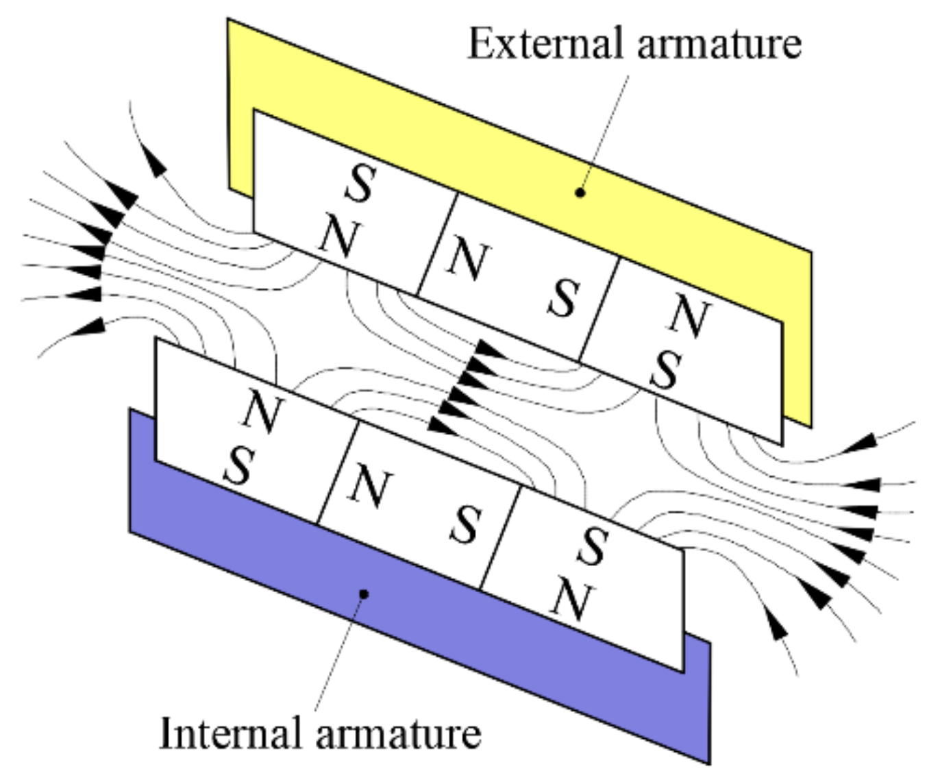
Figure 3.
Schematic diagram of the 2D valve: (a) 2D maglev valve; and (b) 2D mechanical valve.
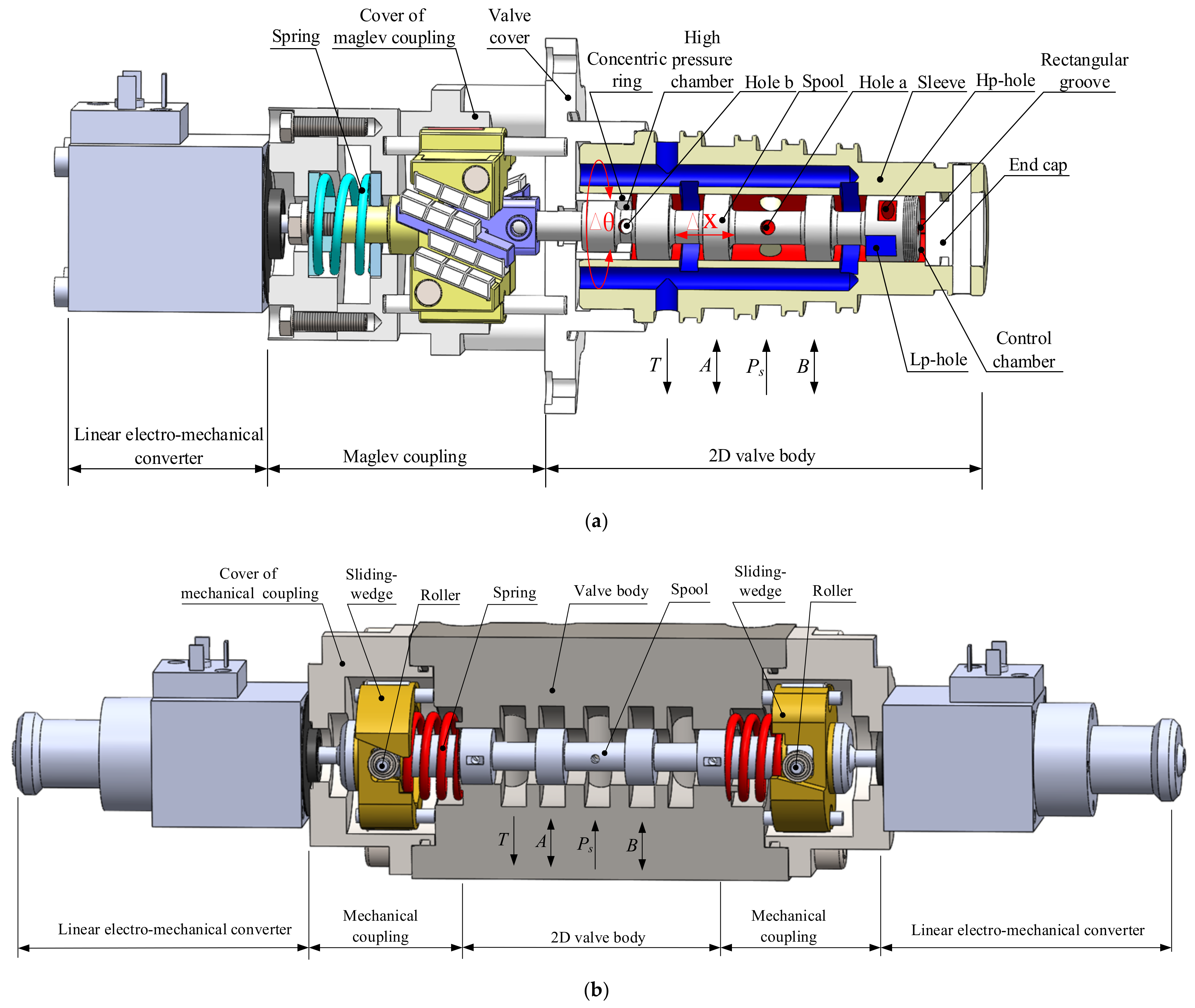
Figure 4.
Force analysis of maglev coupling: (a) front view and rear view when not electrified; (b) front view and rear view when electrified; and (c) side view when electrified.
Figure 4.
Force analysis of maglev coupling: (a) front view and rear view when not electrified; (b) front view and rear view when electrified; and (c) side view when electrified.

Figure 5.
Schematic diagram of infinitesimals of permanent magnet (IPM)-1 and IPM-2.

Figure 6.
Schematic diagram of rectangular–rectangular combinations of permanent magnet units (CPMUs).
Figure 6.
Schematic diagram of rectangular–rectangular combinations of permanent magnet units (CPMUs).
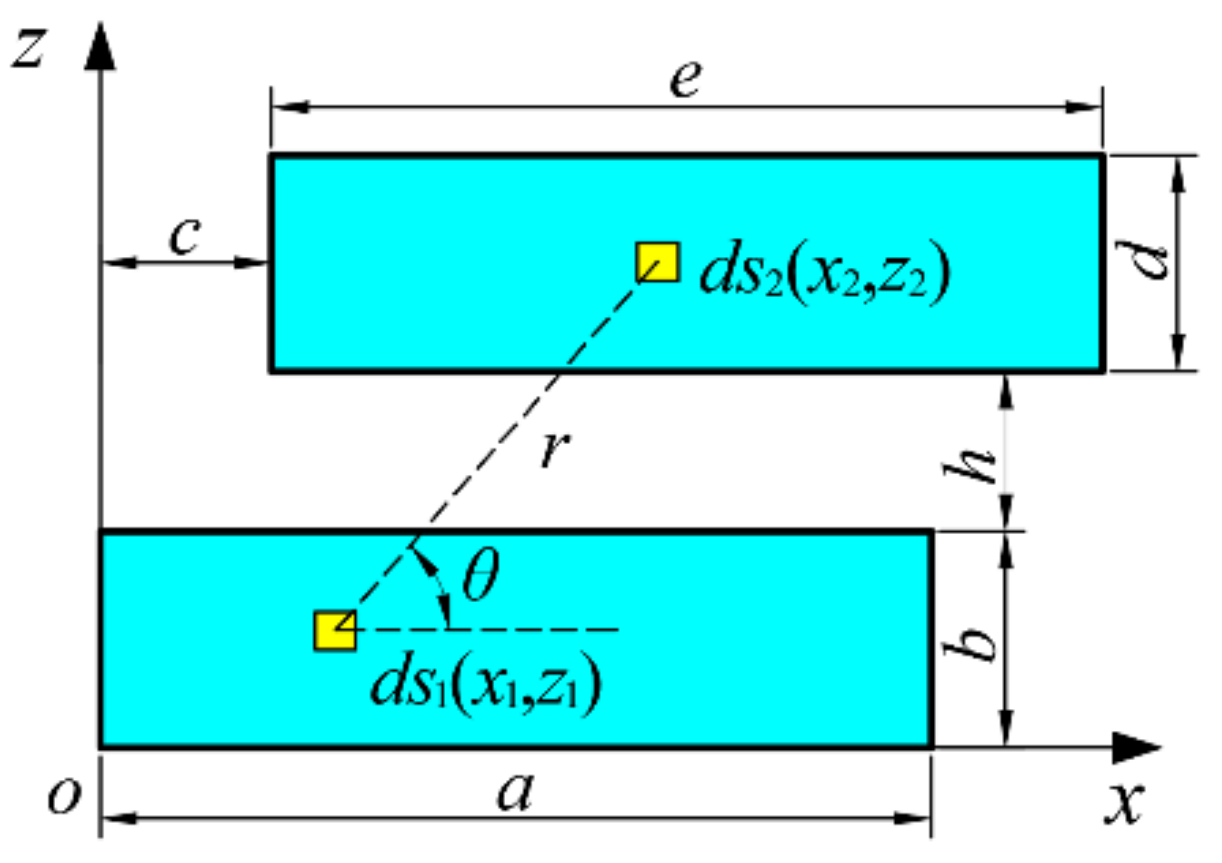
Figure 7.
Schematic diagram of triangular–rectangular CPMUs.
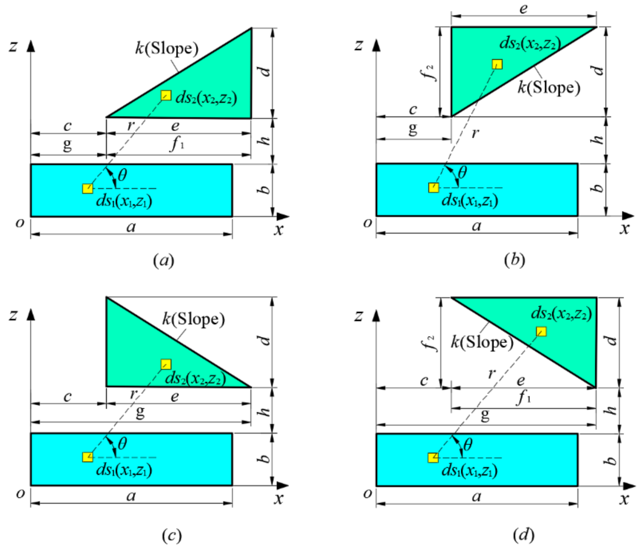
Figure 8.
Schematic diagram of triangular–triangular CPMUs.

Figure 9.
Two opposed Halbach arrays on same side.

Figure 10.
Decomposition of array-1.
Figure 11.
Surface curve of the output torque: (a) = 20°; (b) = 40°; (c) = 60°; and (d) = 80°.
Figure 12.
Relationship between , and .

Figure 13.
Magnetic flux line diagram and contour plot of maglev coupling: (a) = 30°, = 1.22 mm, = 0 mm; (b) = 30°, = 1.22 mm, = 1 mm; (c) = 40°, = 0.35 mm, = 0 mm; (d) = 40 = 0.35 mm, = 1 mm; (e) =50°, = −0.49 mm, = 0 mm; and (f) = 50°, = −0.49 mm, = 1 mm.
Figure 13.
Magnetic flux line diagram and contour plot of maglev coupling: (a) = 30°, = 1.22 mm, = 0 mm; (b) = 30°, = 1.22 mm, = 1 mm; (c) = 40°, = 0.35 mm, = 0 mm; (d) = 40 = 0.35 mm, = 1 mm; (e) =50°, = −0.49 mm, = 0 mm; and (f) = 50°, = −0.49 mm, = 1 mm.


Figure 14.
Verification for the parameter optimization with FEM simulation: (a) influence of on the torque–displacement characteristics with = 30°; (b) influence of on torque–displacement characteristics with = 40°; (c) influence of on torque–displacement characteristics with = 50°.
Figure 14.
Verification for the parameter optimization with FEM simulation: (a) influence of on the torque–displacement characteristics with = 30°; (b) influence of on torque–displacement characteristics with = 40°; (c) influence of on torque–displacement characteristics with = 50°.
Figure 15.
Prototypes of maglev coupling.

Figure 16.
Experimental platform for prototypes of maglev coupling.

Figure 17.
Torque–displacement characteristics of maglev coupling (a) = 30°, = 1.22 mm; (b) = 40°, = 0.35 mm; and (c) = 50°, = −0.49 mm.
Figure 17.
Torque–displacement characteristics of maglev coupling (a) = 30°, = 1.22 mm; (b) = 40°, = 0.35 mm; and (c) = 50°, = −0.49 mm.


Table 1.
Values of triangular–rectangular intermediate parameters.
| Structure | ||||
|---|---|---|---|---|
| (a) | ||||
| (b) | ||||
| (c) | ||||
| (d) |
Table 2.
Values of triangular–triangular intermediate parameters.
| Structure | ||||
|---|---|---|---|---|
| (a) | ||||
| (b) | ||||
| (c) | ||||
| (d) |
Table 3.
Key structural parameters used in the parametric analysis.
| Parameters | Value |
|---|---|
| /(°) | 0 to 90 |
| /(mm) | −5 to 5 |
| /(mm) | 3 |
| /(mm) | 0 to 1 |
| /(T) | 1.19 |
| Lever of force /(mm) | 35 |
| Width of PM /(mm) | 6 |
| Height of PM /(mm) | 3 |
| Length of PM /(mm) | 10 |
Table 4.
Design structure parameters for maglev prototypes.
| Parameters | Value |
|---|---|
| Width × height × length of rectangular PM/(mm) | 6 × 3 × 10 |
| Long width × short width × height × length of 30° trapezoidal PM/(mm) | 7.73 × 6 × 3 × 10 |
| Long width × short width × height × length of 40° trapezoidal PM/(mm) | 8.52 × 6 × 3 × 10 |
| Long width × short width × height × length of 50° trapezoidal PM/(mm) | 9.58 × 6 × 3 × 10 |
| Optimal of 30° maglev coupling/(mm) | 1.22 |
| Optimal of 40° maglev coupling/(mm) | 0.35 |
| Optimal of 50° maglev coupling/(mm) | −0.49 |
| Height of air gap /(mm) | 3 |
| Residual magnetic induction intensity /(T) | 1.19 |
| Coercivity of magnet/(A/m) | 9.15 × 10⁵ |
| Lever of force/(mm) | 35 |
Table 5.
Summary of output torque values.
| 0.5 | 1 | ||
|---|---|---|---|
| Torque/(N·m) ( = 30°, = 1.22 mm) | Analytical | 0.316 | 0.631 |
| FEM | 0.298 | 0.597 | |
| Exp | 0.295 | 0.561 | |
| Difference | 6.65% | 11.09% | |
| Torque/(N·m) ( = 40°, = 0.35 mm) | Analytical | 0.322 | 0.643 |
| FEM | 0.308 | 0.618 | |
| Exp | 0.299 | 0.579 | |
| Difference | 7.14% | 9.95% | |
| Torque/(N·m) ( = 50°, = −0.49 mm) | Analytical | 0.314 | 0.629 |
| FEM | 0.297 | 0.595 | |
| Exp | 0.282 | 0.547 | |
| Difference | 10.19% | 13.04% |
Publisher’s Note: MDPI stays neutral with regard to jurisdictional claims in published maps and institutional affiliations. |
© 2021 by the authors. Licensee MDPI, Basel, Switzerland. This article is an open access article distributed under the terms and conditions of the Creative Commons Attribution (CC BY) license (http://creativecommons.org/licenses/by/4.0/).
Share and Cite
MDPI and ACS Style
Meng, B.; Zhu, C.; Xu, H.; Dai, M.; Li, S. Analytical and Experimental Investigations of Novel Maglev Coupling Based on Opposed Halbach Array for a 2D Valve. Actuators 2021, 10, 61. https://doi.org/10.3390/act10030061
AMA Style
Meng B, Zhu C, Xu H, Dai M, Li S. Analytical and Experimental Investigations of Novel Maglev Coupling Based on Opposed Halbach Array for a 2D Valve. Actuators. 2021; 10(3):61. https://doi.org/10.3390/act10030061
Chicago/Turabian StyleMeng, Bin, Chenhang Zhu, Hao Xu, Mingzhu Dai, and Sheng Li. 2021. "Analytical and Experimental Investigations of Novel Maglev Coupling Based on Opposed Halbach Array for a 2D Valve" Actuators 10, no. 3: 61. https://doi.org/10.3390/act10030061
Note that from the first issue of 2016, this journal uses article numbers instead of page numbers. See further details here.