Parameter Identification of BLDC Motor Using Electromechanical Tests and Recursive Least-Squares Algorithm: Experimental Validation

Abstract

In this article, the parameter identification of a brushless DC motor (BLDC) is presented. The approach here presented is based on a direct identification considering a three-phase line-to-line voltage electromagnetic torque as function of the electric currents and rotor speed. The estimation is divided into two stages. First, the electrical parameters are estimated by well-known no-load and DC tests. Consequently, estimation of mechanical parameters is performed using a recursive Least Square Algorithm. The proposed approach is validated by comparing model responses to motor real time responses. Additionally, the design, digital simulation and real time implementation of a PI rotor speed controller, based on the estimated model, validate the identification proposal presented here.

1. Introduction

The use of permanent magnets (PMs) in electric machines has several advantages over conventional machines, such as the absence of field winding losses, simpler construction, greater efficiency, and higher torque density [1,2]. Additionally, considerable improvements in dynamic performance can be achieved because there is a nearly constant air-gap magnetic flux density in each permanent magnet pole face. Brushless direct current (BLDC) motors use PMs as magnetic field excitation and are widely popular in automotive, aeronautic, industrial, and commercial applications because of reduced mechanical losses, lower maintenance costs and higher reliability compared to brushed motors.

The BLDC motor analyzed in this work has a trapezoidal back-emf waveform, and it is fed by a DC power source through a three-phase power converter. Several strategies have been reported in the literature for the control of BLDC motors such as PID, fuzzy logic, neural networks, optimization via genetic algorithms, and sliding-modes [2,3,4,5,6]. Depending on the application, control schemes may be designed for regulation or tracking of rotor position, speed or torque.

The performance of typical control schemes for BLDC motors relies on information of rotor position and machine parameters. The rotor position is determined via Hall-effect sensors or sensorless techniques, whereas the parameters must be known a priori or determined online [3,7]. These parameters are the winding resistance and inductance, rotor inertia, back-emf constant, and the coefficients of damping or friction [8,9].

Accurate information of parameters is generally not available, and an identification scheme must be formulated. There are several ways to determine motor parameters. However, an accurate estimation is subject to precise design information of the machine such as stator and rotor cores materials as well as their geometry, type of permanent magnets and winding distribution, etc. When this information is available, there are popular methods for determining these parameters such as the classical models of magnetic circuits or finite element analysis (FEA) [10,11,12].

Detailed information on machine design is generally not available. Therefore, experimental tests are usually performed to obtain the parameters listed above [13]. In [9,14,15,16], stator resistance and inductance, rotor inertia and damping coefficient of a DC motor are determined by analyzing its step response to blocked-rotor and no-load tests. In [17], a modified blocked-rotor test is performed to determine the direct and quadrature axes inductances and the back-emf constant of a PM synchronous motor. In [4], the motor is excited with a variable frequency input and the frequency response is fitted to appropriate transfer functions, resulting in the lumped parameters of the model. The main drawback of these tests is that they are performed under very specific circumstances—blocked rotor, zero speed, no load, simplified dynamics—which may not represent the performance of the motor under normal operating conditions. Therefore, the results may need to be refined.

The electrical and mechanical parameters are also subject to variation due to different causes; for example, stator resistance, damping coefficient and PM strength vary with temperature, while inductances vary nonlinearly with the effective air-gap field and damping coefficient varies with rotor speed. These variations are compensated using online identification schemes based on optimization methods and adaptive controllers [3,15,18]. In [18], a method that combines a genetic algorithm and simplex search is used to determine the parameters of the nonlinear friction components in a DC motor. In [3], an algebraic identification method combined with a classical gradient search are used online on a BLDC motor to tune an adaptive speed controller; the model used is a simplified one that neglects the damping coefficient. The results are satisfactory in numerical simulation; however, no experimental validation is provided. In [19], the moment of inertia is estimated dynamically using a state observer to improve the performance of a PI control scheme.

Intelligent strategies such as artificial neural networks, particle swarm and bat algorithms have also been used in determining BLDC parameters [6,20]. However, these works determine the lumped parameters of the transfer functions used in the control design stage rather than the machine parameters. Some of the most used algorithms are based on a least-squares (LS) estimate. This approach compares the measured output with the modeled output and minimizes their difference. Assuming an accurate model, the LS method provides a versatile, efficient, reliable, and easy to implement parameter estimation method [21]. In particular, the recursive least-squares (RLS) is a modified version of the LS that can be implemented online, allowing the use of sizable sets of measurements, and solving the minimization problem using an efficient matrix inversion method [21,22]. These characteristics allow to determine the dynamic model parameters and improve the performance of a linear speed controller [23]. In [2] the RLS algorithm was used to determine nonlinearities of the model, such as Coulomb friction coefficient, back-emf harmonics, and cogging torque coefficients. In [7], the minimum cogging torque coefficients are determined using RLS. In [24], the stator resistances are estimated using the RLS algorithm in a torque ripple minimization scheme.

In previous works, a notable disadvantage is that the number of estimated parameters of the model is limited [9,10,14,24,25], the estimated parameters are typically lumped [6,18,20], or are intended to refine nonlinear behavior of the machine [2,7]. Moreover, the parameter estimation schemes are established as an intermediate step to tune and test controllers. On the other hand, in [4] an estimation of the full model parameters is obtained but makes use of a frequency domain approach, which is less intuitive and is limited by the laboratory equipment available. The aim of this work is to propose an easy, reliable and performable strategy for the entire identification of parameters contained in the dynamic model of a BLDC motor for control purposes, requiring a minimal number of experimental measurements. The method requires only the measurement of two-line voltages and currents and two signals of hall effect position sensors instead of three. The electrical parameters are determined through two tests which are accomplishable using a conventional data acquisition system of electrical signals. The mechanical parameters are determined using the RLS algorithm. For this stage, the electric measurements are used to estimate the instantaneous torque, which in turn is used as input to the RLS algorithm for the mechanical identification. Additionally, the validity of the estimated parameters is assessed against manufacturer information, as well as through numerical simulation using the state space model. Moreover, a real-time implementation of a well-known speed control strategy is presented. Our methodology can be applied for the parameter estimation in other electrical machines, such as brush DC motor, brushless AC, and reluctance machines.

This paper is structured as follows. In Section 2 the model equations and the parameters involved are presented; in Section 3 the tests used to determine the parameters are described alongside a brief description of the RLS algorithm; Section 4 briefly outlines the experimental setup, details the results of the tests comparing with information provided by the manufacturer and their validity is tested. Finally, Section 6 presents the concluding remarks of this work.

2. Mathematical Modeling and Problem Formulation

The BLDC motor is a three-phase machine, whose windings are typically wye-connected. Its dynamic behavior can be described by the following system of equations:

$$\begin{array}{cc}\hfill \mathbf{v}\left(t\right)& =r\mathbf{i}\left(t\right)+\frac{{\mathrm{d}}^{}}{\mathrm{d}{t}^{}}\mathbf{\lambda }\left(t\right),\hfill \end{array}$$

(1a)

$$\begin{array}{cc}\hfill T_e\left(t\right)-T_l\left(t\right)& =J\frac{{\mathrm{d}}^{}}{\mathrm{d}{t}^{}}{\omega }_r\left(t\right)+b{\omega }_r\left(t\right).\hfill \end{array}$$

(1b)

Equation (1a) is a matrix equation that represents the electrical dynamics of the motor. The bold terms $\mathbf{v}$, $\mathbf{i}$ and $\mathbf{\lambda }$ are the voltage, current and flux linkage vectors, and are of the form $\alpha ={\left[{\alpha }_a{\alpha }_b{\alpha }_c\right]}^T$, where $a,b$ and c are the phases of the machine. The first term on the right-hand side of (1a) represents the ohmic voltage drop across the stator phase resistance r, and the second term represents the voltage induced by the time-varying currents. Equation (1b) describes the dynamics of the rotor speed ${\omega }_r$. This is done through the torque balance between the inertial and damping torques—produced by the rotor inertia J and damping coefficient b—with the input electromagnetic torque $T_e$ and load torque $T_l$.

The flux linkages can be modeled by considering linearity in the magnetic core and balanced currents with the expression

$$\begin{array}{c}\hfill \mathbf{\lambda }\left(t\right)=\ell \mathbf{i}\left(t\right)+{\mathbf{\lambda }}_{\mathit{r}}\left(t\right),\end{array}$$

(2)

where the first term on the right-hand side yields the vector of flux linkages due to the magnetic field produced by the stator time-varying currents and the second term is the vector of flux linkages due to relative motion between the stationary stator windings and the rotary PM. The inductance ℓ represents the effect of self and mutual induction in the stator windings carrying balanced currents. The flux linkages due to the magnetic field produced by the PM ${\mathbf{\lambda }}_r$ are, however, dependent on the magnet arrangements and the winding uniform distribution. This is taken into account in [26] by modeling these flux linkages as quadratic functions of rotor position, so that the time-derivative of the flux linkages leads to trapezoidal back-emf waveforms, whose magnitudes are proportional to the rotor speed ${\omega }_r$, the back-emf constant $k_v$ and the number of poles P. The induced voltages due to the rotor-produced flux linkages are

$$\begin{array}{c}\hfill {\mathbf{e}}_r\left(t\right)=\left(\frac{P}{2}\right)k_v{\omega }_r\mathbf{f}\left({\theta }_e\right),\end{array}$$

(3)

where $\mathbf{f}\left({\theta }_e\right)$ is a vector of trapezoidal functions of the rotor position (radians) ${\theta }_e$, with magnitude 1 and phase angle of 120 ${}^{\circ }$. These voltages are referred to as back electromotive force (emf) or internal voltage. Here, as in (1a), this vector has the form $\mathbf{f}={\left[f_a{f}_b{f}_c\right]}^T$.

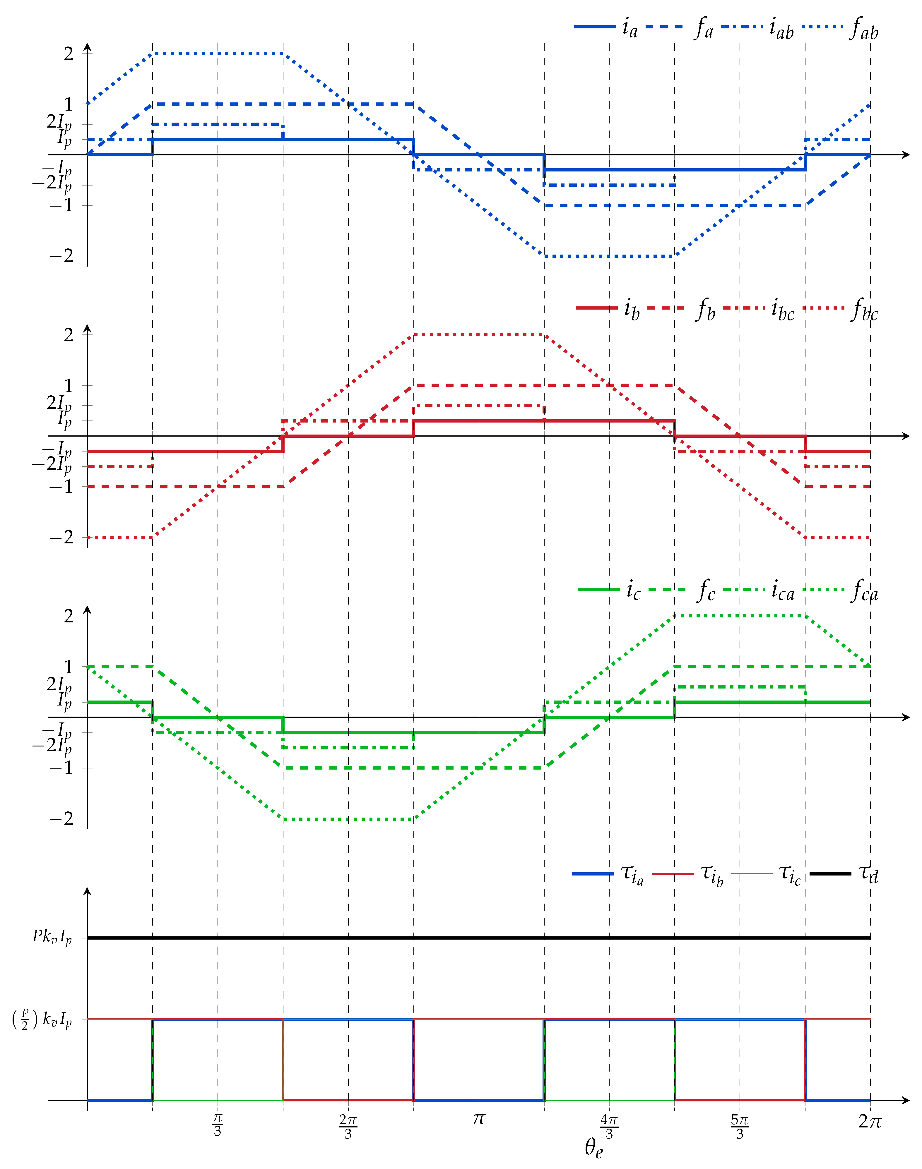
The developed torque is obtained by the vector product

$$\begin{array}{c}\hfill T_e\left(t\right)=\left(\frac{P}{2}\right)k_v{\mathbf{f}}^T\left({\theta }_e\right)\mathbf{i}\left(t\right).\end{array}$$

(4)

The ideal form of $\mathbf{i}$ and $\mathbf{f}$ are shown in Figure 1. It can be observed that the currents are AC square waves of amplitude $I_p$ in discontinuous-current mode, i.e., are zero in 60${}^{\circ }$ intervals and are positive or negative in 120${}^{\circ }$ intervals. This mode of operation is called 120${}^{\circ }$ commutation, and ensures current flows through only two phases at any given time. The flat intervals of the trapezoidal back-emf waveforms correspond to those of the currents and, as a result, a constant torque $T_e\left(t\right)=P{k}_v{I}_p$ is produced (see Figure 1). Nevertheless, as a result of the armature reaction and other parasitic effects, the back-emf waveform is never flat and the developed torque is not constant, but rippled [27].

BLDC Model

Using the expressions derived in previous sections, the mathematical model of a BLDC motor is typically developed under the following assumptions: The power converter that generates the necessary source waveforms is comprised of ideal components, the stator windings are wye-connected and symmetric, the magnetic materials are considered linear, and the ideal current and back-emf waveforms produce a constant torque. Accordingly, Equations (1a) and (1b) take the form

$$\begin{array}{cc}\hfill \mathbf{v}\left(t\right)& =r\mathbf{i}\left(t\right)+\ell \frac{{\mathrm{d}}^{}}{\mathrm{d}{t}^{}}\mathbf{i}\left(t\right)+\left(\frac{P}{2}\right)k_v{\omega }_r\left(t\right)\mathbf{f}\left({\theta }_e\right),\hfill \end{array}$$

(5a)

$$\begin{array}{cc}\hfill \left(\frac{P}{2}\right)k_v{\mathbf{f}}^T\left({\theta }_e\right)\mathbf{i}\left(t\right)& =b{\omega }_r\left(t\right)+J\frac{{\mathrm{d}}^{}}{\mathrm{d}{t}^{}}{\omega }_r\left(t\right)+T_l\left(t\right).\hfill \end{array}$$

(5b)

In most applications, the neutral point of the BLDC is unaccessible and the measurements must be made in a line-to-line basis. The formulation of the BLDC model (line quantities) under these assumptions is therefore [1,28]

$$\begin{array}{cc}\hfill {\mathbf{v}}_L\left(t\right)& =r{\mathbf{i}}_L\left(t\right)+\ell \frac{{\mathrm{d}}^{}}{\mathrm{d}{t}^{}}{\mathbf{i}}_L\left(t\right)+\left(\frac{P}{2}\right)k_v{\omega }_r\left(t\right){\mathbf{f}}_L\left({\theta }_e\right),\hfill \end{array}$$

(6a)

$$\begin{array}{cc}\hfill \left(\frac{P}{2}\right)\left(\frac{k_v}{3}\right){\mathbf{f}}_L^T\left({\theta }_e\right){\mathbf{i}}_L\left(t\right)& =b{\omega }_r\left(t\right)+J\frac{{\mathrm{d}}^{}}{\mathrm{d}{t}^{}}{\omega }_r\left(t\right)+T_l\left(t\right),\hfill \end{array}$$

(6b)

where the vectors with an L subindex are of the form ${\mathbf{\alpha }}_L={\left[{\alpha }_{ab}{\alpha }_{bc}{\alpha }_{ca}\right]}^T$. Note that the line currents in (6) do not have a strict physical meaning as the voltages, but are rather the result of the manipulation of the phase equations. An important consequence of using line quantities in the model is that the winding are no longer in discontinuous-current mode, which means that the current does not return to zero in every period and their magnitudes along with the back-emf waveforms are affected by a factor of 2. These waveforms are also shown in Figure 1. Equation (6) is useful because it naturally provides a 120 ${}^{\circ }$ commutation. In any commutation interval, the two phases conducting x and y are modeled by the voltage equations

$$\begin{array}{c}\hfill v_{xy}\left(t\right)=r{i}_{xy}\left(t\right)+\ell \frac{{\mathrm{d}}^{}}{\mathrm{d}{t}^{}}{i}_{xy}\left(t\right)+\left(\frac{P}{2}\right)k_v{\omega }_r\left(t\right)f_{xy}\left({\theta }_e\right).\end{array}$$

(7)

However, due to the fact that phases x and y are connected in series, the current flowing through them is the same but with opposite signs, i.e., $i_x=-i_y$. Therefore, the following simplification can be made:

$$\begin{array}{c}\hfill v_{xy}=r_t{i}_x\left(t\right)+{\ell }_t\frac{{\mathrm{d}}^{}}{\mathrm{d}{t}^{}}{i}_x\left(t\right)+\left(\frac{P}{2}\right)k_v{\omega }_r\left(t\right)f_{xy}\left({\theta }_e\right),\end{array}$$

(8)

where $r_t=2r$ and ${\ell }_t=2\ell$ are the terminal resistance and inductance, respectively.

3. Electromechanical Tests and Recursive Least-Squares Algorithm

3.1. DC Tests

The resistance and inductance of a BLDC motor can be determined by applying a constant DC voltage across two phases of the machine while blocking the rotor. This is equivalent to making ${\omega }_r=0$ in (8) and $v_{xy}=V_{xy}$ a constant voltage. Assuming an ideal neutral connection [7,29], this convenient setup leads to linear, first-order differential equations for the pair of phases x and y

$$\begin{array}{c}\hfill V_{xy}=r_t{i}_x\left(t\right)+{\ell }_t\frac{{\mathrm{d}}^{}}{\mathrm{d}{t}^{}}{i}_x\left(t\right).\end{array}$$

(9)

The solution of (9) is given by

$$\begin{array}{c}\hfill i_x\left(t\right)=K_e{V}_{xy}\left(1-e^{-\frac{t}{{\tau }_e}}\right)+i_x\left(0\right)e^{-\frac{t}{{\tau }_e}}\end{array}$$

(10)

for an initial condition $i_x\left(0\right)$. $K_e$ and ${\tau }_e$ are the electric steady-state gain and time constant of the circuit. The transient response produced by the exponential terms in (10) can be visualized and measured using a data acquisition system; thus, $r_t$ and ${\ell }_t$ can be determined through

$$\begin{array}{c}\hfill {\widehat{r}}_t=\frac{1}{K_e}=\frac{V_{xy}}{I_x}\mathrm{and}{\widehat{\ell }}_t={\tau }_e{\widehat{r}}_t,\end{array}$$

(11)

where ${\widehat{r}}_t$ and ${\widehat{\ell }}_t$ are the estimates of $r_t$ and ${\ell }_t$, and $I_x$ is the measured steady-state current.

3.2. Open-Circuit Tests

Open-circuit tests are conducted by keeping the armature terminals open-circuited and hence no current flowing in the armature windings. The test is performed by coupling a prime mover to the shaft of the motor and running it at a constant speed. Under these conditions $i_x\left(t\right)=0$ and the back-emf $e_{xy}$ equals the terminal voltage:

$$\begin{array}{c}\hfill v_{xy}\left(t\right)=e_{xy}\left(t\right)=\left(\frac{P}{2}\right)k_v{\mathsf{\Omega }}_r{f}_{xy}\left({\theta }_e\right),\end{array}$$

(12)

where ${\mathsf{\Omega }}_r$ is the steady-state value of the measured rotor speed. If the number of poles is unknown it can be determined by computing the steady-state angular frequency ${\mathsf{\Omega }}_e$ of the induced voltages

$$\begin{array}{c}\hfill P=2\frac{{\mathsf{\Omega }}_e}{{\mathsf{\Omega }}_r}.\end{array}$$

(13)

Let $E_p$ be the peak value of the induced voltages when the prime mover is running at constant speed and recalling that the peak value of the trapezoidal waveforms equals two, the back-emf constant can be determined by

$$\begin{array}{c}\hfill {\widehat{k}}_v=\frac{E_p}{P{\mathsf{\Omega }}_r}.\end{array}$$

(14)

3.3. No-Load Tests

A no-load test consists of starting the motor with no load connected to the shaft ($T_l\left(t\right)=0$). This makes the motor run with near a zero current, thus reducing the armature reaction and making the amplitude of the back-emf close to that of the terminal voltage. Assuming ideal back-emf and current waveforms, the developed torque has a constant value $T_e=P{k}_v{I}_p$, so Equation (5b) can be simplified to

$$\begin{array}{c}\hfill P{k}_v{I}_p=J\frac{{\mathrm{d}}^{}}{\mathrm{d}{t}^{}}{\omega }_r\left(t\right)+b{\omega }_r\left(t\right),\end{array}$$

(15)

which is also a linear, first-order differential equation with solution

$$\begin{array}{c}\hfill {\omega }_r\left(t\right)=P{K}_m{k}_v{I}_p\left(1-e^{-\frac{t}{{\tau }_m}}\right)+{\omega }_r\left(0\right)e^{-\frac{t}{{\tau }_m}},\end{array}$$

(16)

where $K_m$ and ${\tau }_m$ are the mechanical steady-state gain and time constant, respectively. Using a procedure similar to the one described for the determination of resistance and inductance, the damping coefficient and moment of inertia estimates can be obtained with

$$\begin{array}{c}\hfill \widehat{b}=\frac{1}{K_m}\mathrm{and}\widehat{J}={\tau }_m\widehat{b}.\end{array}$$

(17)

Discrete Mechanical Equation

Adhering to the standard notation, let u be the input of a linear system and y its output. The relation between u and y can be represented through the transfer function $G\left(s\right)=Y\left(s\right)/U\left(s\right)$, where U and Y are the Laplace transforms of u and y, respectively. Let us now assume that G represents a first-order system, characterized by a steady-state gain K and a time constant $\tau$, of which the input and output are measured at a definite sample time T. This results in the discrete representation of G considering a zero-order hold in the complex z domain [21,30]

$$\begin{array}{cc}\hfill G\left(z\right)& =\frac{K\left(1-e^{-\frac{T}{\tau }}\right)z^{-1}}{1-e^{-\frac{T}{\tau }}{z}^{-1}}\hfill \end{array}$$

(18)

and the corresponding difference equation of the system

$$\begin{array}{c}\hfill y\left(k\right)=e^{-\frac{T}{\tau }}y\left(k-1\right)+K\left(1-e^{-\frac{T}{\tau }}\right)u\left(k-1\right),\end{array}$$

(19)

where k represents the sampling instant. The mechanical equation of the BLDC model under no-load conditions (15) is a system of this kind; one can thus rewrite (19) making $u=T_e$ and $y={\omega }_r$ as

$$\begin{array}{c}\hfill {\omega }_r\left(k\right)=e^{-\frac{T}{{\tau }_m}}{\omega }_r\left(k-1\right)+K_m\left(1-e^{-\frac{T}{\tau }}\right)T_e\left(k-1\right).\end{array}$$

(20)

Defining the regression vector $\phi$ and the parameter vector $\vartheta$ as

$$\begin{array}{c}\hfill \phi \left(k\right)={\left[{\omega }_r\left(k-1\right)T_e\left(k-1\right)\right]}^T\mathrm{and}\vartheta ={\left[e^{-\frac{T}{{\tau }_m}}{K}_m\left(1-e^{-\frac{T}{{\tau }_m}}\right)\right]}^T,\end{array}$$

(21)

Equation (20) can be recast as

$$\begin{array}{c}\hfill {\omega }_r\left(k\right)={\vartheta }^T\phi \left(k\right).\end{array}$$

(22)

in compact form.

3.4. Recursive Least-Squares Algorithm

A brief description of the RLS algorithm is presented. Equation (22) is composed of past measurements of ${\omega }_r$ and $T_e$; therefore, it assumes certainty in the parameters $\vartheta$. When these parameters are unknown or uncertain, the product ${\vartheta }^T\phi$ may not reproduce the system output ${\omega }_r$. If one defines system output error as the difference between the actual output and the modeled output as follows

$$\begin{array}{c}\hfill \epsilon \left(k\right)={\omega }_r\left(k\right)-{\vartheta }^T\phi \left(k\right),\end{array}$$

(23)

the weighted least-squares criterion applied to (23) can be expressed as the cost function $\mathcal{J}$, defined as

$$\begin{array}{c}\hfill \mathcal{J}=\sum _{k=1}^{N}B\left(N,k\right){\epsilon }^2\left(k\right),\end{array}$$

(24)

where N is the number of samples and B is a weighting function. The parameter vector $\phantom{\vartheta }\widehat{\vartheta }$ that minimizes (24) is defined as the parameter estimates. Determining $\phantom{\vartheta }\widehat{\vartheta }$ involves matrix operations that can be highly costly in computational resources. To avoid this, (24) can be minimized recursively, updating at every sample step with the new information processed from the regression vector $\phi$. This can be achieved by selecting a weighting function of the form

$$\begin{array}{c}\hfill B\left(N,k\right)=\prod _{j=k+1}^N\beta ={\beta }^{N-k},0\le \beta \le 1,\end{array}$$

(25)

where $\beta$ is a constant weight that is recursively multiplied by itself. With this weighting function the RLS algorithm, along with Equation (23), is synthesized as follows:

$$\begin{array}{cc}\hfill \phantom{\vartheta }\widehat{\vartheta }\left(k\right)& =\phantom{\vartheta }\widehat{\vartheta }\left(k-1\right)+\frac{F\left(k-1\right)\phi \left(k\right)\epsilon \left(k\right)}{\beta +{\phi }^T\left(k\right)F\left(k-1\right)\phi \left(k\right)},\hfill \end{array}$$

(26a)

$$\begin{array}{cc}\hfill F\left(k\right)& =\frac{1}{\beta }\left(F\left(k-1\right)-\frac{F\left(k-1\right)\phi \left(k\right){\phi }^T\left(k\right)F\left(k-1\right)}{\beta +{\phi }^T\left(k\right)F\left(k-1\right)\phi \left(k\right)}\right),\hfill \end{array}$$

(26b)

where $\vartheta$ is updated with each sample k and F is a positive defined non-singular matrix, relating the input and output variables. According to (25), older samples are exponentially discarded and a larger weight is given newer ones. For this reason $\beta$ is called forgetting factor. Its impact on the algorithm can be interpreted as a noise sensibility parameter: A smaller $\beta$ helps the algorithm to converge faster but becomes highly sensible to noise. The necessary steps to obtain (26) are rather involved, however, the detailed methodology is reported in [21,22]. The recursive nature of this algorithm allows an online implementation to adaptively adjust the parameters fed into controllers or observers.

The input signal fed to the algorithm must satisfy the condition of persistent excitation to yield optimal results [4,21,24]. That is, input signal must satisfy the persistent excitation condition to ensure that all process modes or dynamics are activated, and to ensure that the covariance matrix F remains non-singular which implies an input signal with an appropriate frequency sweep. This means that the input signal must be a “white noise”, which is difficult to achieve in practice. However, this condition can be relaxed by ensuring that the input signal keeps the system response out of steady state condition at all times. Resulting from the limitations of the experimental setup, the tests for numerical identification were made by using a piecewise constant input signal that produces transients at regular intervals but does not excite every mode of the system. The algorithm uses the calculated torque as input and the rotor speed as output to identify the parameters of Equation (15).

4. Experimental Setup and Results

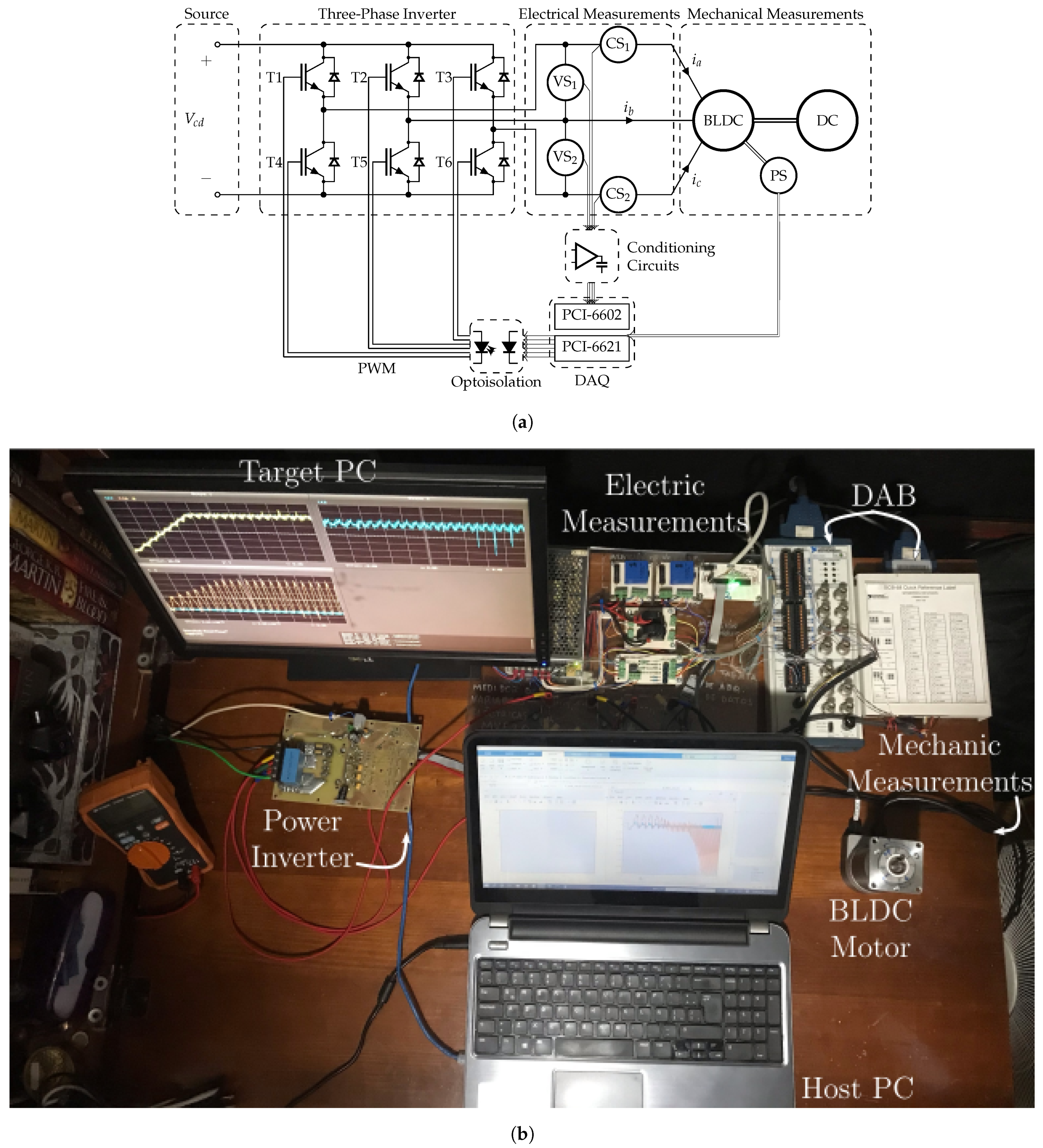
Several tests were performed on a four pole BLDC motor of known parameters. Two voltage and two current sensors were used to measure the line voltages ($v_{ab}$ and $v_{cb}$) and currents ($i_a$ and $i_b$). The rotor position and speed were measured using two Hall-effect sensors and an incremental encoder. The three-phase waveforms that power the BLDC were generated using a three-phase IGBT-based inverter. The electrical signals were measured using a National Instruments analog data-acquisition board (DAB), labeled PCI-6602 in Figure 2a, and the signals of the incremental encoder using a National Instruments digital DAB, labeled PCI-6621 in Figure 2a. The latter was also used to generate the gate signals to drive the inverter according to the algorithms programmed in Simulink for the no-load tests and the PI control validation tests. The schematic diagram is is shown in Figure 2. The voltage, current and position sensors are labeled VS${}_x$, CS${}_x$ and PS, respectively. Additional components are shown in Figure 2, such as conditioning circuits for the electrical signals, an optoisolation stage to separate the logical stage from the power stage, and a DC machine mechanically coupled to the BLDC motor for the open-circuit tests. The measured data was acquired and analyzed using Simulink Real-Time, Simulink, and MATLAB, from The Mathworks, Inc. The sample time of voltage, current and Hall-effect sensors was $T=125 \mathsf{\mu }\mathrm{s}$.

4.1. Resistance and Inductance Estimation

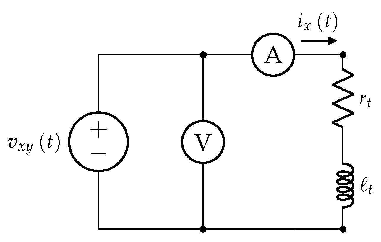
To determine the terminal resistance $r_t$ and inductance ${\ell }_t$ of the BLDC motor, a constant DC voltage was applied to two terminals of the motor and the voltage and current were measured. This setup is shown in Figure 3.

This test was performed for the three phases and different values of $V_{xy}$. The applied voltages were limited by the rated current of the motor and the power source used. The current $I_x$ flowing through the phases connected to the power source was measured and used to determine the electric steady-state $K_e$ and the terminal resistance $r_t$ using (11). The time constant ${\tau }_e$ was determined using the data-acquisition system and was used along with the terminal resistance to compute the terminal inductance ${\ell }_t$ for each phase using (11).

Table 1. Results for the resistance and inductance estimation tests.

Test	Measured Values			Computed Values
	${\mathit{V}}_{\mathbf{xy}}$ [V]	${\mathit{I}}_{\mathit{x}}$ [A]	${\mathit{\tau }}_{\mathit{e}}$ [s]	${\mathit{r}}_{\mathit{x}}$ [$\mathsf{\Omega }$]	${\mathit{r}}_{\mathit{t}}$ [$\mathsf{\Omega }$]	${\mathit{\ell }}_{\mathit{t}}$ [mH]
1	5.4	3.4	1.75	1.59	1.19	2.08
2	3.49	2.19	1.81	1.59	1.19	2.16
3	−3.47	−2.18	1.95	1.59	1.19	2.32
4	−5.21	−3.28	1.97	1.59	1.19	2.34
5	5.34	3.36	1.61	1.59	1.19	1.91
6	3.42	2.17	1.73	1.58	1.18	2.05
7	−3.29	−2.09	1.81	1.58	1.18	2.13
8	−5.08	−3.22	1.91	1.58	1.18	2.24
9	5.42	3.44	2.03	1.58	1.18	2.39
10	2.88	1.82	2.06	1.58	1.18	2.42
11	−2.88	−1.81	1.77	1.59	1.19	2.1
12	−5.06	−3.22	1.66	1.57	1.17	1.94
Mean value					1.18	2.17
Uncertainty					0.0056	0.0601

show the measured voltage, current and time constant. The fourth column shows the resistance $r_x$ computed using (11) and the values shown in the second and third columns. The fifth column shows the terminal resistance value computed by subtracting from $r_x$ the resistance of the wires used to connect the elements of the circuit, which equals $0.4\pm 0.0038 \mathsf{\Omega }$. The last column shows the value of inductance computed from each test using (11). The resulting parameters for each test were averaged to yield the estimated values ${\widehat{r}}_t$ and ${\widehat{\ell }}_t$ and the corresponding uncertainties were computed as the standard error for the number of tests performed. These results are shown in the bottom rows of Table 1.

The results were substituted in Equation (10) and compared with the experimental results. This is shown graphically in Figure 4: The measured current for three of these tests is displayed with continuous lines. The dashed lines are the results obtained by substituting the determined parameters in (10) along with the corresponding measured voltage. For each test, a shaded area is shown, which represents the response within the uncertainty intervals.

It can be seen that the experimental results are into these intervals for the first-order approximation (9) for time values above ${\tau }_e=1.28 \mathrm{m}\mathrm{s}$. Below this time, neither response falls within the expected estimated region. As can be seen in the Figure 4, the experimental curves are those of a higher order dynamic system, which reveals the deficiencies of the first-order model approximation used in this test. This difference is due to dynamics, such as magnetic nonlinearity, or the rotor position, that are not considered in the utilized model. Regarding the rotor position, it is worth mentioning that the tests were performed by letting the rotor align itself to the field produced by driving current through the windings under study and locking it in that position. So for each phase the tests were made in similar conditions regarding the initial position of the rotor and the respective magnetic flux path.

4.2. Back-emf Constant

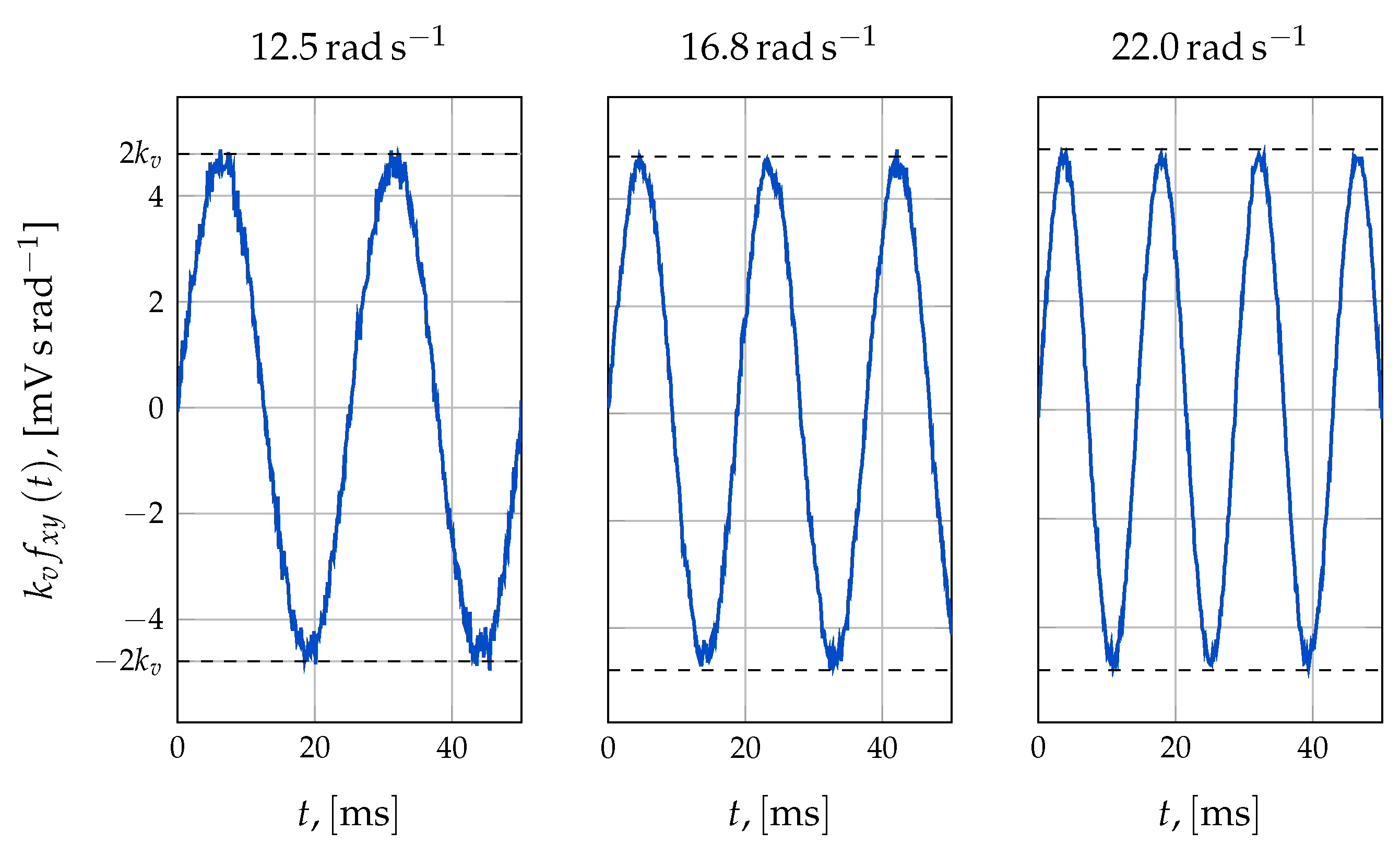
The procedure described in the previous section for the open-circuit test was performed by coupling a controlled DC motor to the shaft of the BLDC motor. The line voltages were measured using voltage sensors and the speed was determined with an incremental encoder. Figure 5 shows the results of this test at different speeds, (12, 16, and 22 $\mathrm{rad}/\mathrm{s}$) displaying the obtained voltage measurements $e_{xy}$ divided by the steady-state rotor speed ${\mathsf{\Omega }}_e$ of the respective test, i.e.,

$$\begin{array}{c}\hfill \frac{e_{xy}\left(t\right)}{{\mathsf{\Omega }}_e\left(t\right)}=k_v{f}_{xy}\left({\theta }_e\right).\end{array}$$

(27)

It can be readily seen that the waveforms have the same amplitude regardless of the speed, as expected, from the fact that the shape functions have fixed amplitudes. It can also be seen that the waveforms are not ideally trapezoidal. This is due that the waveform is heavily dependent upon how the PMs are arranged in the machine and not every magnet array yields the trapezoidal back-emf shown in Figure 1. In addition to this the measured quantities are line voltages, so the flat-top intervals are shorter (cf. Figure 1). For each test, the peak values of the generated voltages were averaged to determine the amplitude of the induced voltages $E_p$, the rotor speed ${\mathsf{\Omega }}_r$ was measured, and the back-emf constant was determined by substituting these values and the number of poles $P=4$ in (14). The results from every test are shown in

Table 2. Results for the back-emf constant estimation tests.

Test	Measured Values		Computed Values
	${\mathit{E}}_{\mathit{p}}$ [V]	${\mathsf{\Omega }}_{\mathit{r}}$ [rad s${}^{-1}$]	${\mathit{k}}_{\mathit{v}}$ [mV s rad s${}^{-1}$]
1	1.21	12.53	24.16
2	1.40	14.56	24.00
3	1.61	16.78	24.01
4	1.84	19.15	23.95
5	2.02	21.05	23.93
6	2.11	22.03	23.90
Mean value			23.99
Uncertainty			0.0377

. The last column shows the back-emf constant for each test computed using (14). As before, the estimated parameter was obtained by averaging these values, and the uncertainty was computed as the standard error. The estimated parameter during this test is shown in the bottom rows of Table 2.

4.3. Moment of Inertia and Damping Coefficient Estimation Using RLS

A no-load test was conducted to determine the mechanical parameters of the motor. The test consisted of starting the motor from standstill to a speed within its operating range. This was achieved by sensing the rotor position and determining the commutation logic to turn on the corresponding phase sequentially. The magnitude of the applied voltage was determined by the well-known volts per hertz relationship, used in scalar control strategies for induction motors. The speed was varied at equal time intervals for 6 $\mathrm{s}$. The input torque was calculated using the current and rotor position measurements and Equation (4). However, because of the sampling rate, the non-ideal waveforms and the measurement noise, the resultant torque was excessively noisy. This poses a problem regarding the RLS algorithm, because of the first-order approximation used. The torque signal was therefore smoothed using a moving median filter prior to being input to the algorithm. This smoothing strategy was chosen to remove as much outliers as possible from the torque signal by taking the median of windows of 100 samples, without significantly affecting its dynamics.

The setup for the RLS identification algorithm considers the following values

$$\begin{array}{c}\hfill \beta =0.92,T=1.25 \mathsf{\mu }\mathrm{s},\phantom{\vartheta }{\widehat{\vartheta }}_0={\left[0.10.1\right]}^T,F_0=\left[\begin{array}{cc}50& 0\\ 0& 50\end{array}\right].\end{array}$$

(28)

There is no standard methodology for choosing a forgetting factor. In general, values close to 1 are rapidly convergent but very noise-sensitive. This tradeoff was considered in the choice of $\beta$, which was tuned after several trials on the algorithm using the input torque data. The sample time was selected considering that the measurement of the Hall-effect sensors used in the commutation algorithm was acquired using the same board as the voltage and current measurements. The initial parameters $\phantom{\vartheta }{\widehat{\vartheta }}_0$ were chosen arbitrarily as well as the initial correlation matrix $F_0$, which was required to be positive definite.

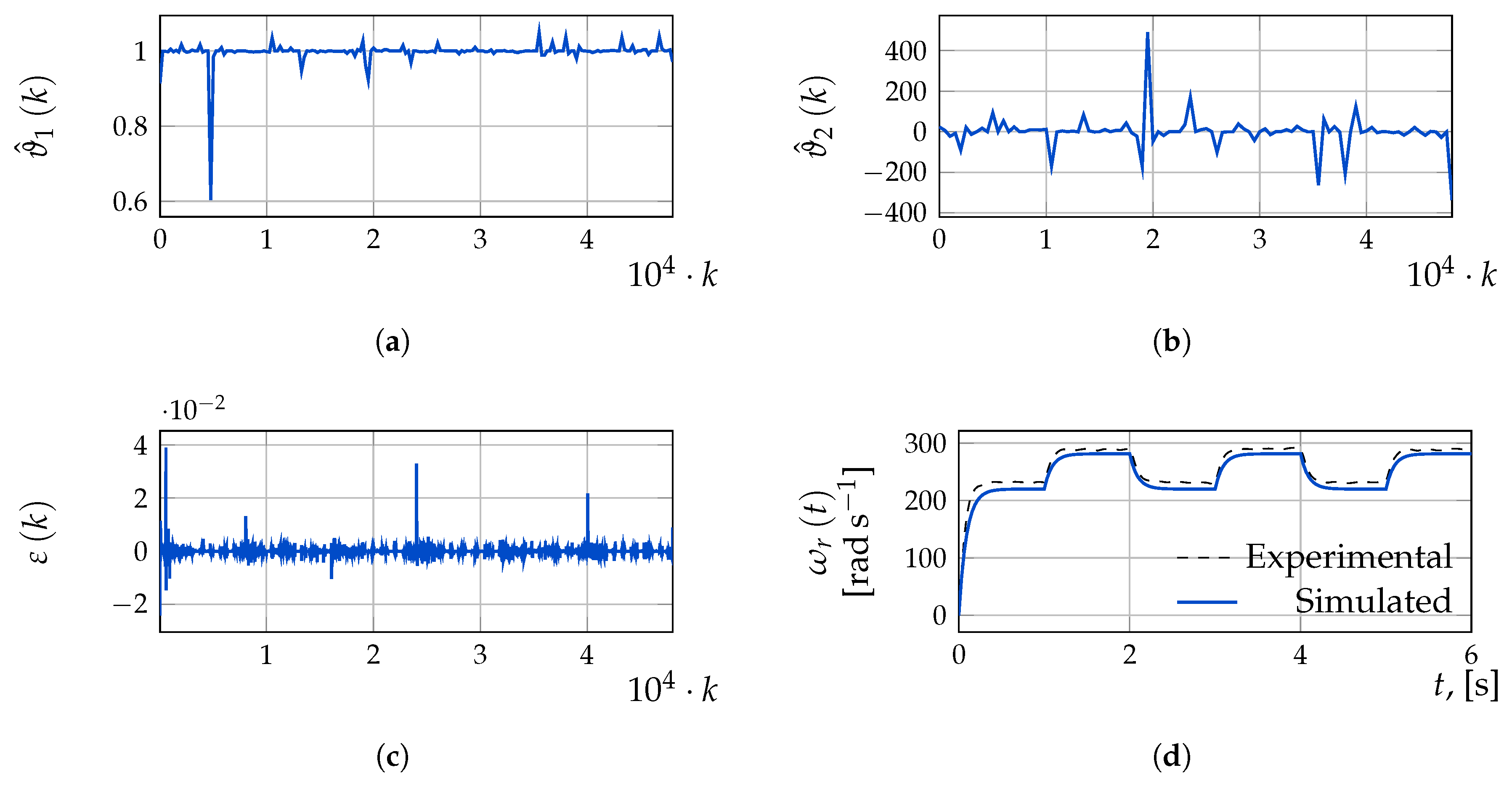
Using this configuration and the filtered torque signal, the algorithm was run to determine the discrete parameters $\phantom{\vartheta }{\widehat{\vartheta }}_1$ and $\phantom{\vartheta }{\widehat{\vartheta }}_2$ (these results are shown in Figure 6). Figure 6a,b show the parameter trajectory during the test where both signals can be seen to have a significant noise component. Nevertheless, a trend can be established by eliminating the outliers in the resulting data. Figure 6c shows the output error $\epsilon$ for the test. It can be seen that the algorithm tends to minimize the output error despite the parameters are not converging to a constant value. The mean values of the obtained parameters are:

$$\begin{array}{c}\hfill \phantom{\vartheta }\widehat{\vartheta }={\left[\phantom{\vartheta }{\widehat{\vartheta }}_1\phantom{\vartheta }{\widehat{\vartheta }}_2\right]}^T={\left[0.99868.1069\right]}^T.\end{array}$$

(29)

Substituting these parameters into Equation (18) and running the algorithm using an input torque of the same magnitude as the measured torque yields a very approximate output speed compared to the measured one, however, a steady-state error can be appreciated during the whole tests, which reveals a poor estimate of the parameter ${\vartheta }_2$ and, by extension, of the damping coefficient. In fact, this parameter is the one that most differs from the expected value, as presented in Section 4.4.1. This is shown in Figure 6d.

Solving (21) for $K_m$ and ${\tau }_m$, these parameters are given by:

$$\begin{array}{c}\hfill {\tau }_m=-\frac{T}{ln\left(\phantom{\vartheta }{\widehat{\vartheta }}_1\right)}\mathrm{and}{K}_m=\frac{\phantom{\vartheta }{\widehat{\vartheta }}_2}{1-\phantom{\vartheta }{\widehat{\vartheta }}_1},\end{array}$$

(30)

and the moment of inertia and the damping coefficient are in turn given by (17). Substituting (29) into (30) and (17), the estimated mechanical parameters are shown in

Table 3. Results for the damping coefficient and moment of inertia tests.

Parameter	Units	Value	Uncertainty
			Value	%
Damping coefficient, b	$\mathsf{\mu }\mathrm{N}\mathrm{m} {\mathrm{s}}^{-1}$	172.69	21.42	12.40
Moment of inertia, J	$\mathrm{g} \mathrm{c}{\mathrm{m}}^2$	154.04	28.58	18.55

.

$$\begin{array}{c}\hfill \widehat{b}=172.69\pm 21.42 \mathsf{\mu }\mathrm{N}\mathrm{m} {\mathrm{s}}^{-1}\mathrm{and}\widehat{J}=154.04\pm 28.58 \mathrm{g} \mathrm{c}{\mathrm{m}}^2.\end{array}$$

(31)

4.4. Validation

In this section the validity of the estimated parameters is assessed.

4.4.1. Manufacturer Data

All the obtained parameters are summarized in

Table 4. Parameters provided by the manufacturer and estimated through tests.

Parameter	Units	Manufacturer		Estimation		Discrepancy, %
		Value	Tolerance, %	Value	Uncertainty, %
Resistance, r	$\mathsf{\Omega }$	1.18	10	1.1826	0.48	0.22
Inductance, ℓ	$\mathrm{m}\mathrm{H}$	2.30	15	2.0369	12.9	11.44
Back-emf constant, $k_v$	$\mathrm{m}\mathrm{V} {\mathrm{s}}^{-1}$	21.96	10	23.994	0.16	9.26
Damping coefficient, b	$\mathsf{\mu }\mathrm{N}\mathrm{m} {\mathrm{s}}^{-1}$	25.62	2.6	172.69	12.4	574.04
Moment of inertia, J	$\mathrm{g} \mathrm{c}{\mathrm{m}}^2$	176.00	20	154.04	18.5	12.47

, along with the parameters provided by the manufacturer. It can be seen that, except for the damping coefficient, all parameters were determined within the uncertainty bounds of both the manufacturer data and the estimated data. The discrepancy in the value of the damping coefficient may be due to several different reasons: The manufacturer employed a different model than the one used in this work, the motor used during these tests was in service for several years and it may have suffered damages or alterations, the friction model comprised very specific operating regimes, such as no-load, same initial conditions for every test and unidirectional rotation, amongst others. Besides, friction phenomena are known to be non-linear and dependent on many factors besides the ones that were modeled in this work. Therefore, the value of the estimated damping coefficient should only be considered valid under the conditions in which the tests were performed.

5. Application Example: Closed-Loop Speed Control

Parameters are needed to tune the controllers of a motor appropriately. Therefore, the obtained parameters were used in the simulation and implementation of a well-known, two-stage PI speed controller [7,26]. That is, the control system is based on an inner loop, which controls the current to generate the required torque and an outer loop to control the speed of the rotor. Both feedbacks were designed using the models of the identified electrical and mechanical subsystems. A BLDC motor was simulated and controlled using the estimated parameters and the controller was tuned to follow a speed trajectory within rated operational ranges of the motor.

The test for evaluating the controller performance consisted of a tracking problem. The speed was raised from 0 to 100 $\mathrm{rad}$/$\mathrm{s}$ following a smooth curve, it then was held constant for two more seconds, and then it was varied sinusoidally with a period of 1 s for four seconds. The controller was tuned using the simulated machine and the resulting gains were implemented in the real-time application for the BLDC motor. Figure 7 shows the results of the test: The desired speed trajectory ${\omega }_r^{\star }$, the measured speed and the simulated speed. It can be seen that the three curves show a very small tracking error even in the most aggressive transients. The measured current is also plotted to show that the rated current is never reached during the whole test.

6. Conclusions

The proposed tests for determining the parameters of a BLDC motor yielded results that are in close agreement with the expected parameter values within reasonable margins of uncertainty. The tests were systematically presented and are reproducible, which means they can be applied to BLDC motors of similar characteristics.The use of the recursive least-squares algorithm applied to the first-order approximation of the mechanical subsystem of the motor is a viable method for estimating the mechanical parameters within margins of uncertainty. However, there exists the drawback of preprocessing the torque input signal. The obtained parameters are able to model the motor in a range of frequencies within the nominal operating limits, so that the dynamic model considered and the first-order approximation are useful for identification and control purposes.

The following abbreviations are used in this manuscript: