
Load Emulation with Independent Metering for a Pump Test Bench

1
Department of Transmission and Drive Technology, Faculty of Mechanical Engineering and Marine Engineering, University of Rostock, Justus-von-Liebig-Weg 6, 18059 Rostock, Germany
2
Hydraulik Nord Technologies GmbH, Ludwigsluster Chaussee 5, 19370 Parchim, Germany
*
Authors to whom correspondence should be addressed.
Actuators 2023, 12(11), 413; https://doi.org/10.3390/act12110413
Submission received: 29 September 2023
/
Revised: 25 October 2023
/
Accepted: 31 October 2023
/
Published: 5 November 2023
(This article belongs to the Special Issue Innovative and Intelligent Actuation for Heavy-Duty Applications)
Abstract
:For the investigation of new types of internal gear pumps under realistic conditions, a test bench is presented that enables dynamic load emulation via the pressure with simultaneous dynamic speed control of the pump. For pressure control, a hydraulic half-bridge with separate control edges is used on both sides of the pump and a pressure control is presented. An error-based adaptive controller is used for pressure control and tested experimentally. It is shown that the error-based adaptive controller has a better performance compared to a simple PID control.
1. Introduction
The trend towards the electrification has not only affected the automotive sector, but also the field of mobile machinery. The electrification of hydraulic drive technology offers the possibility of developing new drive architectures that increase the efficiency of the machines [1]. Energy savings can be achieved by replacing the lossy conventional valve control with variable-speed displacement control [2,3]. In particular, systems with variable-speed fixed displacement pumps have a higher efficiency than constant-speed displacement controls with variable displacement pumps, especially in the part-load range at low to medium pressures and at full load [3,4]. In [5], energy savings of up to 50% compared to conventional hydraulic drives for a bend press are reported. Something similar is reported in the field of mobile machines in [2]. Here, energy consumption was also reduced by up to 50% compared to conventional valve-controlled load sensing systems for a 1 t excavator. If variable-speed fixed displacement pumps are operated in a highly dynamic manner, such systems can have comparable control dynamics to systems with control valves [4]. If the pumps are furthermore operated in the high-speed range, this can increase the power density [6]. In order to meet these requirements for dynamics and speed, such systems are preferably operated with permanently excited synchronous machines [4]. One challenge is to guarantee the durability of the pumps under a large number of dynamic load changes or changed thermal conditions [3]. Tribological problems can occur, especially at low speeds and high pressures [7]. Dynamic test benches are needed to investigate these effects. In [8], an HiL test bench for hydraulic transformers is presented to investigate the performance of the control of hydraulic transformers under realistic dynamic loads. The load emulation is carried out here via the so-called load emulation valve (LEV) by means of a 4/3-way valve, and it replaces the physical load. The aim of the load emulation is to specify the pressure as dynamically as possible. The pressure setpoints of the test bench described in [8] are calculated in real time using an HiL model. In order to investigate the influence of dynamic changes of pressure and speed even in tribologically critical operating modes, this paper presents a test benches that operates the newly developed pumps, especially internal gear pumps, under realistic conditions by dynamically applying speed and pressure to the pump in all four quadrants. Measurements of pressure and speed curves on real machines are used for this purpose. In a further expansion stage, HiL models of real machines and their hydraulic circuits are to be used to determine the feedback effects on the pumps that occur in the machines in order to imprint these on the pumps under test on the test bench. In order to achieve realistic conditions, these feedback effects must be adjusted on the test bench with high dynamics and precision. A permanently excited synchronous motor (PMSM), operated by a frequency converter, drives the pump. Hydraulic load emulation is achieved by dynamic and independent pressurisation on both sides of the pump under test. Especially for the pressurisation, a system architecture and a pressure control are presented and the performance is evaluated on the basis of real measurements. A challenge is the dynamic pressure control in a large operating range with simple, direct operated proportional spool valves without position feedback. Furthermore, the test bench must be able to implement dynamic changes in the direction of rotation of the pump, whereby the pressure control should be as unaffected as possible. Due to the generally strong non-linear behaviour of hydraulic systems, this should be taken into account in the control strategy.
2. Test Bench
In the present configuration of the test bench, the reference signals for pressure and speed are specified via a test cycle. In the future, the test bench will be expanded by adding an HiL model. To test the pump under realistic conditions, the test cycle can be derived from measured values of the pressure and the speed of real applications. The main components of the test bench can be seen in Figure 1. The most important subsystems are the drive system, the load emulating unit (LEU), and the real-time control, where all input and output signals are processed.
Figure 2 shows the LEU and the drive system of the test bench. As shown in Figure 2, the four valves of the LEU are not integrated in a common valve manifold, but are installed in individual valve housings and connected with hose lines. The LEU is also connected to the pump under test with hoses. The pressure transmitters are placed directly in front of the pump under test. To allow any trapped air to escape from the valves and the pressure transmitters, they are installed upside-down.
The mechanical drive of the pump to be tested is realised via a permanently excited synchronous machine, which is operated on a frequency converter. The frequency converter allows both motor and generator operation. A torque measuring system is applied to the drive shaft. The control of the valves, the reading of the sensors, as well as the communication with the frequency converter are carried out via a central real-time capable control. The control operates with a sampling rate of 4 kHz. The control algorithm is executed on a target PC and programmed via a C++ development environment. The load emulation is implemented with four identical valves. Based on the designation from [8], the unit for load emulation is called load emulation unit (LEU) in the following. The LEU is a hydraulic bridge circuit and is supplied via a constant pressure source. A detailed hydraulic circuit scheme is shown in Section 2.1. The pressure specification from the test cycle describes the differential pressure at the pump and must be converted accordingly to the individual pressures on both sides of the pump. Since a four-quadrant operation takes place, both the differential pressure and the speed can assume negative values.
The pressure difference between side A and B is defined with . It is further determined that the pump pumps from side A to B for positive speed n of the pump shaft; thus, the following applies:
Figure 3 shows the definition of the quadrants used in this paper.
Due to the minimum pressure drop across the valves and a minimum pressure each side of to avoid cavitation, the upper and lower areas marked in red cannot be used. The areas were determined numerically with the help of the valve flow map. Static operation with a constant supply pressure of was assumed for the calculation. The quadrants for motoring are restricted by the valve characteristics, since a minimum pressure drops across the valves on the high-pressure side and on the low-pressure side.
2.1. Hydraulic System
The detailed hydraulic circuit is shown in Figure 4. The tested pump in the center is pressurized and supplied by a hydraulic half-bridge marked in red on both side A and B. Four directly controlled proportional spool valves are used to build up the independent metering hydraulic full-bridge. The valves are all normally open. This was implemented for safety reasons in order to open the valves in the event of a fault and to cause a pressure drop in the half-bridges by eliminating the currents in the valve coils.
Both hydraulic half-bridges are supplied with a fixed speed constant pump. The supply flow is . The supply pressure is limited by a mechanical pressure relief valve. The supply flow is selected to be more than the sum of the two flows into the half-bridges, which causes the pressure relief valve to open and set a supply pressure of about . The supply flow is designed on the basis of the displacement and the required operating speed in the tests of the tested pump. An internal gear pump with a constant displacement volume of is examined on the test bench on a variable-speed servo drive. Four pressure transducers are integrated. The pressures and are measured on both sides of the test pump. In front of the hydraulic full-bridge, the supply pressure is measured and also serves to monitor the pressure source. In the event of a fault, the pump under test can, thus, be stopped immediately. The return pressure is measured between the full-bridge and the oil cooler. The oil temperature is also measured at this point. A water–oil plate heat exchanger is installed in the return line to cool the oil. Two check valves, and , are installed on each side of the pump, which act as suction valves in the event of a fault. The pressure relief valves and protect the chambers from overpressure. The individual components are connected with hose lines, which lower the bulk modulus and reduce the stiffness of the system [4].
2.2. Design of the Load Emulating Unit (LEU)
As mentioned above, a hydraulic half-bridge has been realised for load emulation on both sides of the pump (side A and B) with decoupled meter-in and meter-out valves. The method of independent metering for valve-controlled hydraulic drives is often investigated to increase the efficiency of cylinder drives, such as, for example, in [9,10]. The advantages for the application of the separated control edges as load emulator are the high flexibility, the possibility to use advanced control methods, and the comparatively simple valves [11]. The high flexibility enables pressure and flow control [4]. It must also be possible to control the pressure when the pump is at a standstill (). This is where the advantage of the additional degree of freedom due to independent metering becomes apparent. As described in [12], with one continuous degree of freedom, which is the case without independent metering, the pressure-signal gain in case of zero overlap is infinite when there is no flow to the consumer. It is also said that this would place extremely high demands on the proportional valve in order to still allow the pressure holding operation. In [12], it is further explained that the gains and the bypass flow can be flexibly adjusted with two continuous degrees of freedom and, thus, a negative overlap can be set analogous to a conventional 4/3-way valve. This idea will be taken up and examined on the basis of the steady-state valve characteristic gains in the following.
By linearising the valve Equations at the operating point , we obtain for the meter-in valve (5) and for the meter-out valve (6).
The partial derivatives describe the flow-signal gains and the flow-pressure gains at the operating point of the valves. The change of pressure drop across the valve AP is given by . Since the pressure does not change, this results in and, thus, the change of the pressure drop of valve AP is given by . The pressure drop across valve AT is given by . With , the change in pressure drop results in .
With the assumption that both valves are controlled contrary to each other and with and derived above, (5) and (6) lead to (7) and (8).
For a simplified assumption, the same change of flow occurs through both valves , which is the case if there is no change of flow through the pump. Equation (9) shows the pressure-signal sensitivity of a hydraulic half-bridge.
If the flow through the pump is , an analogy to a valve spool with negative overlap is necessary so that the pressure is controllable; otherwise, the pressure is not controllable because . Consequently, neither of the two valves must be closed under steady-state conditions. To realise this, a bypass flow is specified. The advantage of independent metering is that the bypass flow can be adjusted via the software by means of the additional degree of freedom. By varying the bypass flow, the operating point can be shifted to adjust the current pressure-signal sensitivity of the half-bridge.
A relationship between pressure-signal gain and bypass flow also exists with conventional 4/3-way valves. When there is no flow to the consumer, the pressure-signal gain in case of zero overlap is infinite. With a negative overlap, the pressure-signal gain decreases and, in addition, a bypass flow from the supply to the tank occurs within the valve spool. If the negative overlap is increased, this leads to a further decrease in the pressure-signal sensitivity and an increase in the bypass flow. With conventional valve spools, however, the overlap is fixed by design and cannot be changed during operation.
The hydraulic full-bridge is supplied by a pressure source that provides a maximum supply flow of . Therefore, it must be observed that the flows via the half-bridges do not exceed the maximum flow in total. In addition, it has been specified that the hydraulic half-bridges may only be flowed through in one direction. Four identical directly controlled proportional spool valves were used. The proportional solenoids are controlled via pulse width modulation (PWM). The valves have no position feedback and, due to the friction of the valve spool, a hysteresis of about 4%, depending on the parameterisation of the dither signal.
2.3. System Analysis
In hydraulic drive systems, several nonlinearities can be found that should be taken into account in the control [4]. One important non-linearity is the valve characteristic [13]. The valve sensitivity coefficients directly influence the system behaviour [14,15]. The flow-signal gain directly influences the system gain and the flow-pressure gain directly influences the system damping [13,14]. The static and dynamic valve characteristics were investigated experimentally. The static valve flow map was measured with a separate experimental setup. The evaluation showed that the valve characteristics differ from the usual orifice equation, so the flow map was interpolated numerically. Figure 5 shows the flow map after numerical interpolation. The input signal u represents the position of the valve spool, which is determined by the electric current of the valve coil under steady-state conditions. The electric current is proportional to the input signal u. At , the nominal current of the valve coil is present; means no current is applied to the valve coil.
With the help of this flow map, the partial derivatives can be calculated numerically. Figure 6 shows the numerically determined partial derivatives of the flow map.
The numerical derivations were carried out in MATLAB ® using the central-difference method. The flow-signal gain is negative because the valve is normally open. The flow-pressure gain shows a significant change over the operating range. This shows a significant non-linearity of the hydraulic system. To investigate the dynamic behaviour of the valve spool, the valve was examined in its disassembled state with a laser vibrometer. The laser vibrometer was used to measure the position of the valve spool. Since the oil in the valve was cooler than in operation and no flow forces were acting, this test only serves as an estimate of the dynamic behaviour. However, the comparison with literature values showed that the measured valve dynamics are plausible. The valve mechanics show first-order lag (PT1) behaviour with a time constant of about . The static friction of the valve spool was already visible through the hysteresis in the measurement of the flow map. In the disassembled state, it could be determined that the valve spool requires about 5% of the control signal u to break free. This introduces a further non-linearity into the system.
In the following, a linear lumped parameter model for the hydraulic half-bridge on side A is derived, as shown in Figure 7. Assuming that the speed of the pump under test is unaffected by the pressure, the system analysis of a half-bridge should be sufficient.
The pressure drop across valve AP is given by and across valve AT . The hydraulic capacity is defined by a volume V and a bulk modulus and represents the hose line from the half-bridge to the pump and the compressibility of the oil. The charge flow into the chamber is given by , the flow through the valves is given by and , and the flow to the tested pump is given by q. The Laplace transform of the equilibrium of flows is given by Equation (10). The Laplace transform of the pressure build up in the hydraulic capacity is given by (11). The valve flow maps are linearised and also Laplace transformed; see (12) and (13). In all Laplace-transformed equations, s is the Laplace variable. With the linearisation at the point , the valve sensitivity coefficients are obtained by the partial derivatives. These are the flow-pressure gains and and the flow-signal gains and for valve AP and AT.
With the assumption that the flow through the tested pump is not changing, with Equations (10)–(13), the multiple-input single-output transfer Function (14) is derived.
By setting and, thus, coupling the valves, the single-input single-output transfer Function (15) results.
By , as the valves are normally open, the transfer function will be positive. With and , Equation (16) is derived.
The valve dynamics are estimated with a time constant of :
According to the system model in Equation (19), it is obvious that the open loop system is overdamped and, thus, not able to oscillate. In addition to the non-linear flow characteristics of the valves described above, other non-linearities were identified that presumably significantly influence the system behaviour. These are:
- Change of compressibility with pressure [14];
- Valve actuator force limitation;
- Saturation of the valves;
- Static and kinetic friction in the valves leading to hysteresis;
- Limited supply flow.
The change of viscosity with oil temperature [14,16] and the possible associated change in valve spool damping is another time-varying non-linearity, but the change of the temperature is slow compared to the dynamic pressure changes. The effective bulk modulus, which determines the hydraulic capacity, is a large uncertainty and can change significantly, not only in terms of pressure, but also in the case of entrained air and the effective elasticity of the hose lines and hydraulic component housings [14].
2.4. Control Design
The aim of the controller is to ensure highly dynamic pressure control by means of low-cost valves, which makes it possible to map realistic pressure trajectories from test cycles. At the same time, the control performance is to be maintained over as large a range as possible in the quadrant field.
An overview of control methods in hydraulics and how to deal with the nonlinearities common in hydraulics is given in [13]. Due to the nonlinearities, a classical PID controller is always a compromise, which is why various forms of gain scheduling have been proposed [13]. Various adaptive controllers and nonlinear controllers have also been developed to compensate for the nonlinear effects at the various operating points [13,17].
In [18], an error-based adaptive controller (E-BAC), is presented, which enables the control of a non-linear system with a PI controller. It was also shown that, compared to a fixed PI controller, the E-BAC allows no or only a small overshoot and has a shorter rise time. The controller algorithm is described linguistically in [18]. If the control error is large, the proportional gain is increased while the integral gain is decreased, so that the system is underdamped for large errors. If the control error is small, the proportional gain is lowered and the integral gain is increased, so that the system is overdamped. The changes in the gain, depending on the control error, are continuous. In [18], various functions are proposed for this.
Figure 8 shows the structure of the pressure controller used here.
The pressure controller consists of a static feedforward and an adaptive PID controller. For the static feedforward control, the inverse flow maps of the used valves were determined experimentally and stored as a look-up table in the control software. The part of the flow of the pump q through the valve AP, respectively, or the valve AT result from the pump speed n, respectively, or the rotational direction. Together with the specified bypass flow , this results in the setpoint flows and for both valves. The differential pressures of both valves AP and AT result from the pressure setpoint , taking into account the supply pressure and the tank pressure . With the pressure setpoints and and the flow setpoints and , a control signal can, thus, be assigned for each valve. There is a pressure controller for each side of the test pump, which controls the two valves in the same way in opposite directions. In order to take the operating point-dependent non-linearity into account, an error-based adaptive controller (E-BAC), similar to the one in [18], is used. The adaptive gains for the pressure controller of the LEU are a function of the current error e. All gain functions are based on the gaussian function and have been modified for the application, as Equations (20)–(22) show. The proportional gain is determined by Equation (20). The function is characterised with the three parameters, , , and b. The integral gain is computed using Equation (21) with the parameters and b. The derivative gain is calculated with Equation (22) with the parameters and b. Figure 9 shows the gain functions used in the experiments.
The parameter b determines the “sharpness” of the function. The change of the integrator part depending on the control error implies an anti-windup method. If the integrator gain function goes to 0 for large control errors e, the integrator is stopped. The parameters shown in Table 2 were determined experimentally.
3. Experimental Results
For measuring the performance of the pressure control, only the half-bridge on side A is shown here. Pressure steps of 50 and 100 bar each were made at different speeds in pump and motor mode. In addition, the behaviour of the controller at a constant pressure setpoint and changing speed was determined experimentally. The experimentally determined maximum rotational acceleration at a pressure difference of 100 bar is about 17,500 rpm/s, whereby the servo machine is shortly operated in the overload range for this. Table 1 shows the parameters used for the different controllers.
As a comparison of the E-BAC controller with the fixed PID controller, the gains of the E-BAC controller in Table 1 are given for an error . Table 2 shows the parameters used for the gain functions.
3.1. Control Performance
In the following, pressure steps on side A of 50 bar and 100 bar, each at a speed of , and , are shown. The E-BAC controller is compared with a fixed PID-Controller with anti-windup. The same reference value curves are used for both controllers. The two reference value curves and are, therefore, overlaid in the figures. Figure 10 shows a comparison of the two controllers at a pressure step of 50 bar and a speed of . The fixed PID-Controller is designed for a 100 bar step at , as in Figure 11. The design target of the fixed PID-Controller is a fast response, but with the disadvantage of a overshoot. For the initial design of the PID controller, the PID tuning rules based on the ITAE (integral of time-multiplied absolute value of error) criterion described in [17] were applied. The parameters were then further optimised on the test bench, due to the widely varying operating points here. Figure 12 shows a pressure step of 50 bar at a speed of . The measured step responses show that the system behaves differently depending on whether the pump sucks out of the half-bridge or pumps into the half-bridge. This can be clearly seen in the comparison of Figure 11 and Figure 13. The pressure step in Figure 11 has a slightly larger rise time, but a smaller overshoot or, in the case of the E-BAC controller, no overshoot. In this case, the pump sucks from the half-bridge. The pressure step in Figure 13, on the other hand, shows a smaller rise time and a larger overshoot for both controllers. Here, the pump pumps into the half-bridge. One reason for the different system response may be the time behaviour of the flow through valve AP, which dominates the pressure build-up when the pump sucks out of the half-bridge. The time behaviour is presumably determined by the dynamics of the pressure relief valve and by the hose lines in front of the LEU. The control signals and are mostly at the limits during pressure build-up with the E-BAC controller, indicating that the maximum of pressure dynamics are reached with these valves and this system configuration.
Figure 14 shows a speed change from 1000 rpm to 2000 rpm at a rotational acceleration of about 17,500 rpm/s with a constant pressure setpoint of 20 bar.
The initial pressure drop due to the speed increase is about 5 bar lower with the E-BAC controller. The settle time is also lower with the E-BAC controller than with the conventional fixed PID controller.
3.2. Test Cycle
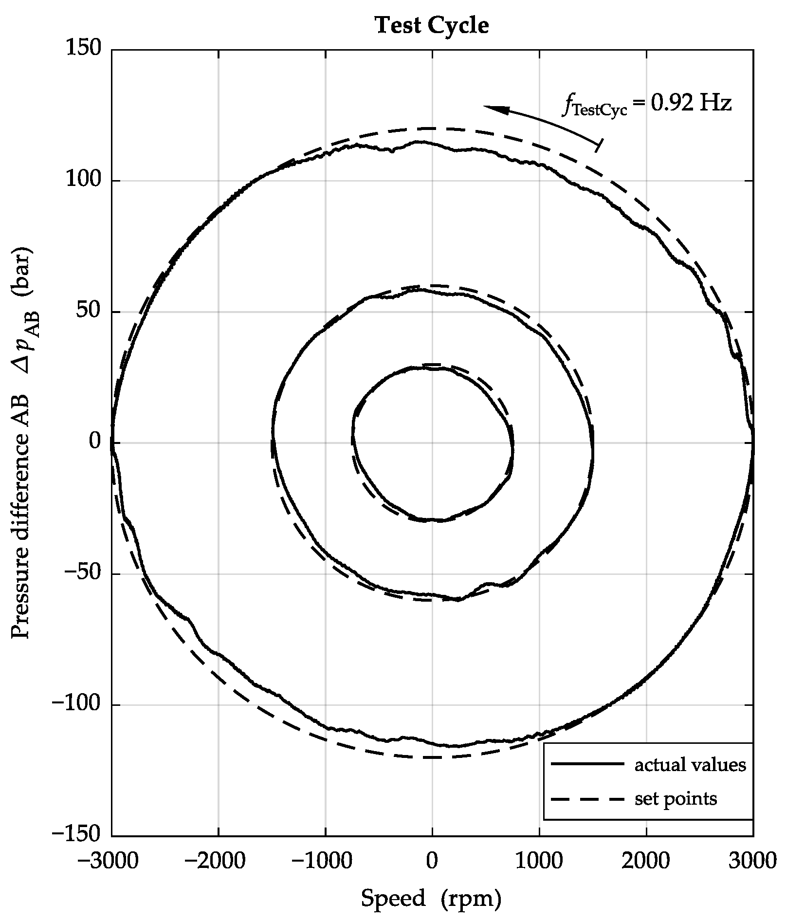
Figure 15 shows a test cycle in which the speed and pressure are changed in all four quadrants. Only the E-BAC controller was activated to control the pressure.
This test cycle was designed such that the outer trajectory reaches approximately the maximum rotational acceleration of about 17,500 rpm/s with a frequency of . The two inner circles are passed through at the same frequency. Due to the lower rates of change of pressure and speed, the errors between the setpoints and actual values are smaller.
4. Discussion
It is experimentally shown that the E-BAC PID pressure controller performs better than a conventional PID controller with anti-windup. The E-BAC PID controller remains stable despite more aggressive settings. The settings of the E-BAC still lead to an overshoot, which, however, is smaller compared to the PID controller. The described pressure control is used to imprint pressure curves measured on real machines or given by an HiL model with high dynamics on a test pump. The pressure curves determined in this way serve as setpoints and typically do not contain any steps. The results in Figure 15 are considered representative for such pressure curves. Even with high dynamics, the control error typically remains below 8 bar. This makes it possible to test the pumps under realistic conditions. Future extension of the test bench in terms of performance and functionality is envisaged. In order to be able to run tests at higher speeds, the flow of the supply must be increased. The use of two or more valves in parallel allows operation at higher flow rates and, thus, at higher speeds. Active electronic pressure control of the pressure source with a pressure transducer and a proportional valve can improve the pressure dynamics. To increase the dynamics of the used valves, an attempt can be made to overload the valve coils for a short time with more than the maximum allowable current in order to increase the magnetic force during dynamic actuation processes. In the next stage of development, the test bench shall be HiL-capable to be able to run model-based realistic tests more efficiently and run more flexible test scenarios.
Author Contributions
Conceptualisation, M.P., T.P., A.B. and J.F.; methodology, M.P.; software, M.P. and J.F.; validation, M.P., T.P., A.B. and J.F.; formal analysis, M.P.; investigation, M.P.; resources, J.F.; data curation, M.P.; writing—original draft preparation, M.P.; writing—review and editing, M.P., T.P., A.B. and J.F.; visualisation, M.P.; supervision, J.F.; project administration, T.P., A.B. and J.F.; funding acquisition, T.P., A.B. and J.F. All authors have read and agreed to the published version of the manuscript.
Funding
This research was funded by the European Regional Development Fund (EFRE) grant number TBI-V-1-431-VBW-146.
Data Availability Statement
Data are not available due to private policy.
Conflicts of Interest
The authors declare no conflict of interest.
References
- Pietrzyk, T. Entwicklung Einer Hochdrehzahl-Innenzahnradpumpe für die Elektrifizierung Mobiler Anwendungen am Beispiel Einer Autarken Dezentralen Elektro-Hydraulischen Achse, 1st ed.; Reihe Fluidtechnik; Shaker: Düren, Germany, 2022; Volume 109. [Google Scholar]
- Casoli, P.; Scolari, F.; Minav, T.; Rundo, M. Comparative Energy Analysis of a Load Sensing System and a Zonal Hydraulics for a 9-Tonne Excavator. Actuators 2020, 9, 39. [Google Scholar] [CrossRef]
- Speicher, T. Methoden zur Auslegung und Effizienzbewertung von drehzahlvariablen Zahnradpumpenaggregaten unter Berücksichtigung von Systemwechselwirkungen. Ph.D. Thesis, Technischen Universität, Kaiserslautern, Germany, 2021. [Google Scholar]
- Gebhardt, N.; Weber, J. Hydraulik—Fluid-Mechatronik; Springer: Berlin/Heidelberg, Germany, 2020. [Google Scholar] [CrossRef]
- Chmiel, M. Drehzahlvariable Pumpenantriebe Halbieren Energiebedarf von Abkantpressen. MM MaschinenMarkt, 26 October 2010. [Google Scholar]
- Pietrzyk, T.; Roth, D.; Schmitz, K.; Jacobs, G. Design study of a high speed power unit for electro hydraulic actuators (EHA) in mobile applications. In Proceedings of the 11th International Fluid Power Conference, Aachen, Germany, 19–21 March 2018. [Google Scholar] [CrossRef]
- Lovrec, D.; Kastrevc, M.; Ulaga, S. Electro-hydraulic load sensing with a speed-controlled hydraulic supply system on forming-machines. Int. J. Adv. Manuf. Technol. 2009, 41, 1066–1075. [Google Scholar] [CrossRef]
- Lee, S.; Li, P.Y. A Hardware-In-The-Loop (HIL) Testbed for Hydraulic Transformers Research. In Fluid Power in the Digital Age: Proceedings of the 15th Scandinavian International Conference on Fluid Power, SICFP’17, Linköping, Sweden, 7–9 June 2017; Krus, P., Ericson, L., Sethson, M., Eds.; Linköping University Electronic Press: Linköping, Sweden, 2017. [Google Scholar]
- Yao, B.; Liu, S. Energy-saving control of hydraulic systems with novel programmable valves. In Proceedings of the 4th World Congress on Intelligent Control and Automation (Cat. No.02EX527), Shanghai, China, 10–14 June 2002; Volume 4, pp. 3219–3223. [Google Scholar] [CrossRef]
- Lyu, L.; Chen, Z.; Yao, B. Energy Saving Motion Control of Independent Metering Valves and Pump Combined Hydraulic System. IEEE/ASME Trans. Mechatron. 2019, 24, 1909–1920. [Google Scholar] [CrossRef]
- Abuowda, K.; Okhotnikov, I.; Noroozi, S.; Godfrey, P.; Dupac, M. A review of electrohydraulic independent metering technology. ISA Trans. 2020, 98, 364–381. [Google Scholar] [CrossRef] [PubMed]
- Kolks, G.; Weber, J. Getrennte Steuerkanten für den Einsatz in stationärhydraulischen Antrieben. O+P Fluidtechnik, 13 June 2018; 42–51. [Google Scholar]
- Edge, K.A. The control of fluid power systems-responding to the challenges. Proc. Inst. Mech. Eng. Part I J. Syst. Control Eng. 1997, 211, 91–110. [Google Scholar] [CrossRef]
- Jelali, M. Hydraulic Servo-systems: Modelling, Identification and Control; Advances in Industrial Control Series; Springer: London, UK, 2003. [Google Scholar] [CrossRef]
- Merritt, H.E. Hydraulic Control Systems; John Wiley and Sons: Hoboken, NJ, USA, 1967. [Google Scholar]
- Manring, N.D.; Fales, R.C. Hydraulic Control Systems, 2nd ed.; Wiley: Hoboken, NJ, USA, 2020. [Google Scholar]
- Liermann, M. Pid Tuning Rule for Pressure Control Applications. Int. J. Fluid Power 2013, 14, 7–15. [Google Scholar] [CrossRef]
- Song, K.Y.; Gupta, M.M.; Jena, D.; Subudhi, B. Design of a robust neuro-controller for complex dynamic systems. In Proceedings of the 2009 Annual Meeting of the North American Fuzzy Information Processing Society (NAFIPS 2009), Cincinnati, OH, USA, 14–17 June 2009; pp. 1–5. [Google Scholar] [CrossRef]
Figure 1.
Main components of the test bench. 1—development environment, 2—target-PC, 3—I/O - terminal, 4—LEU, 5—pump under test, 6—torque measuring system, 7—PMSM, 8—encoder, 9—frequency converter.
Figure 1.
Main components of the test bench. 1—development environment, 2—target-PC, 3—I/O - terminal, 4—LEU, 5—pump under test, 6—torque measuring system, 7—PMSM, 8—encoder, 9—frequency converter.
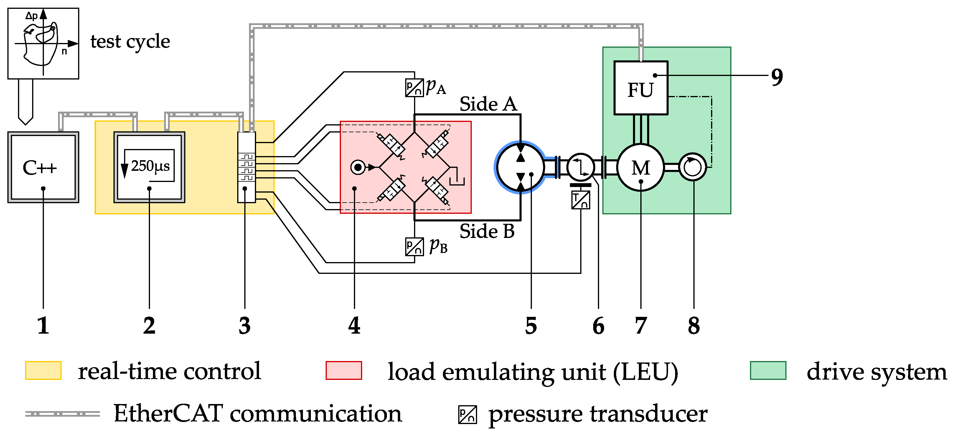
Figure 2.
Real assembly of the test bench with the main components. 5—pump under test, 6—torque measuring system, 7—PMSM.
Figure 2.
Real assembly of the test bench with the main components. 5—pump under test, 6—torque measuring system, 7—PMSM.
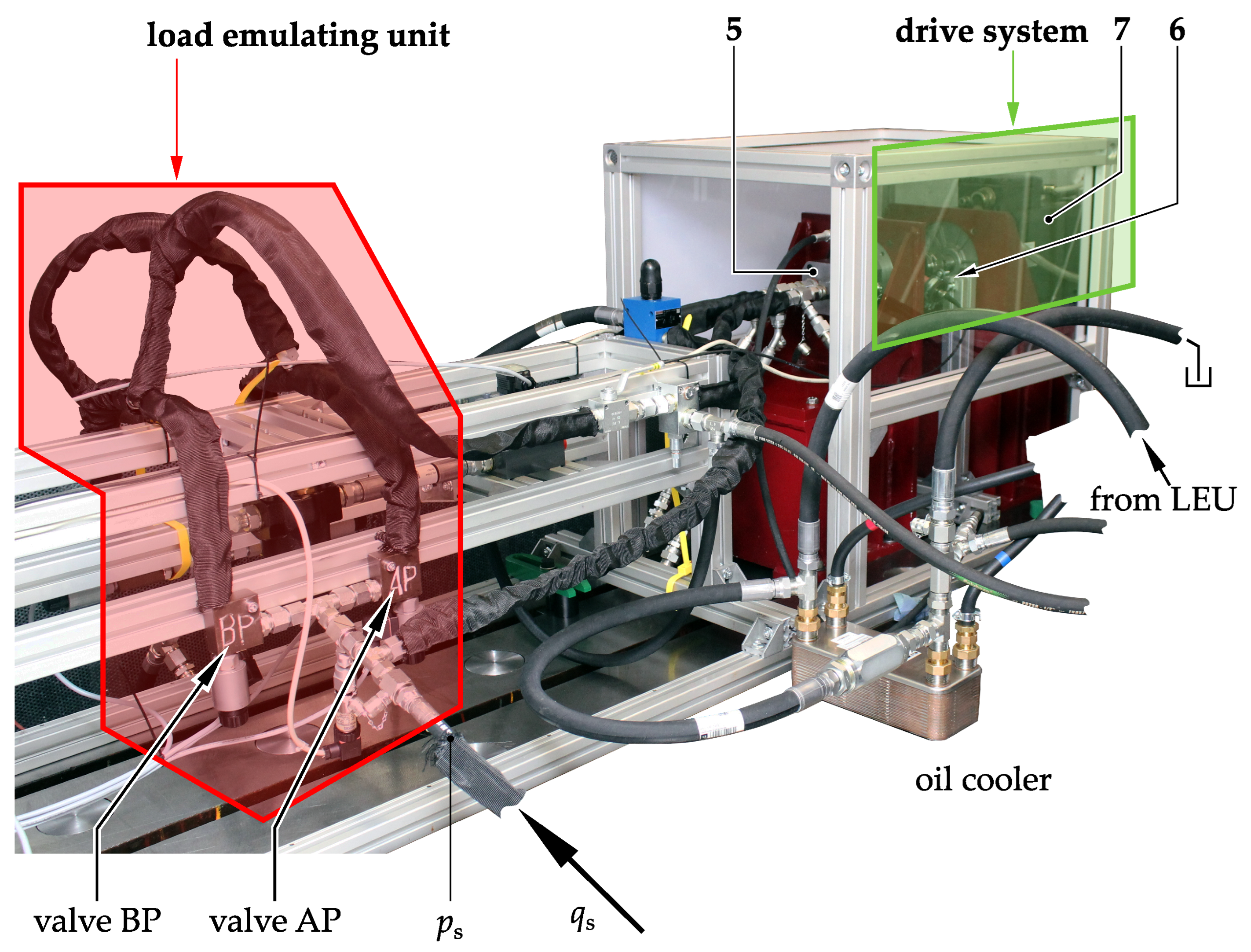
Figure 3.
Definition of the quadrants.
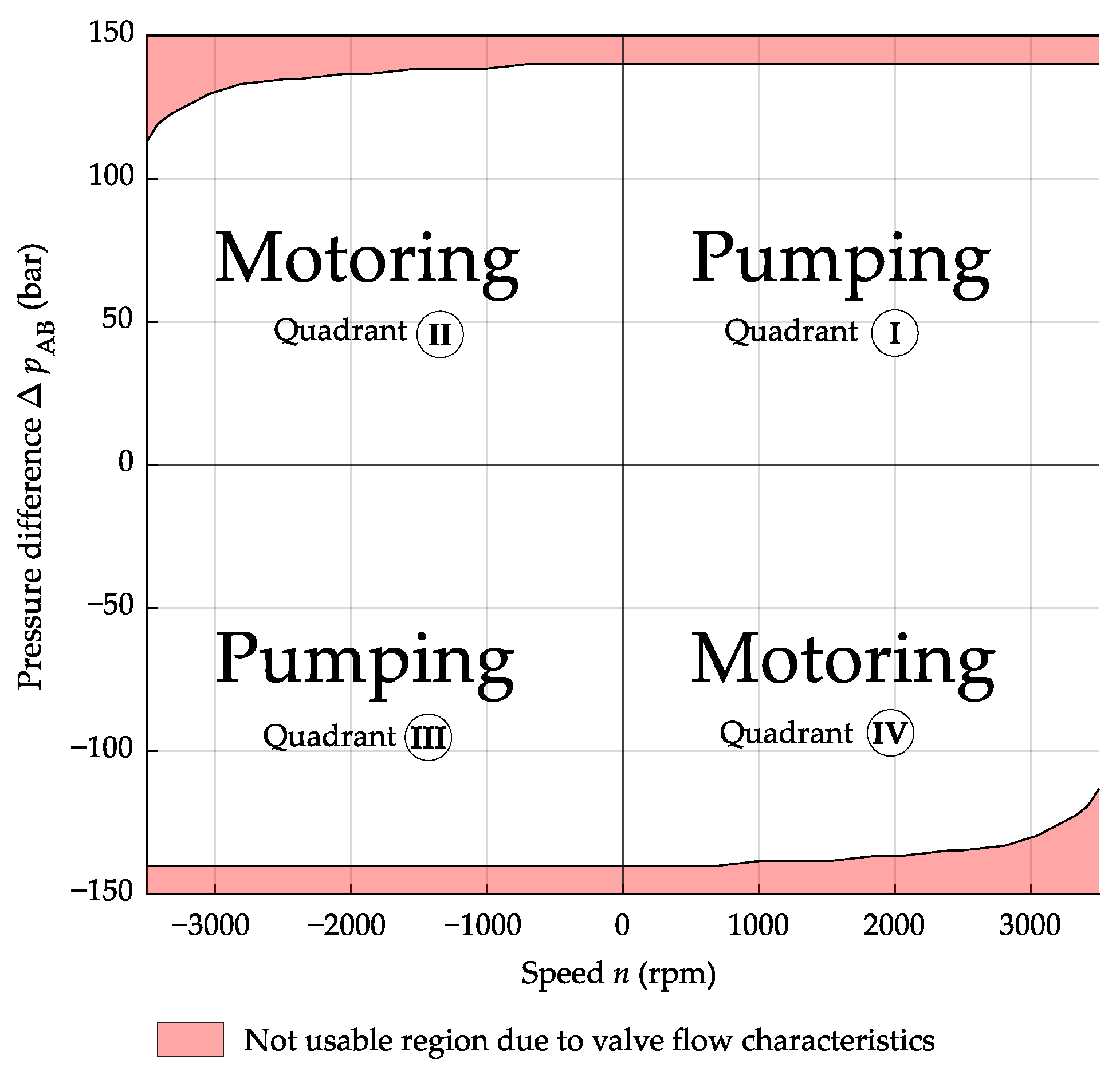
Figure 4.
Scheme of the hydraulic circuit of the test bench.

Figure 5.
Experimentally determined flow map of the used valves.

Figure 6.
Gains derived from flow map: (a) flow-signal gain, (b) flow-pressure gain.
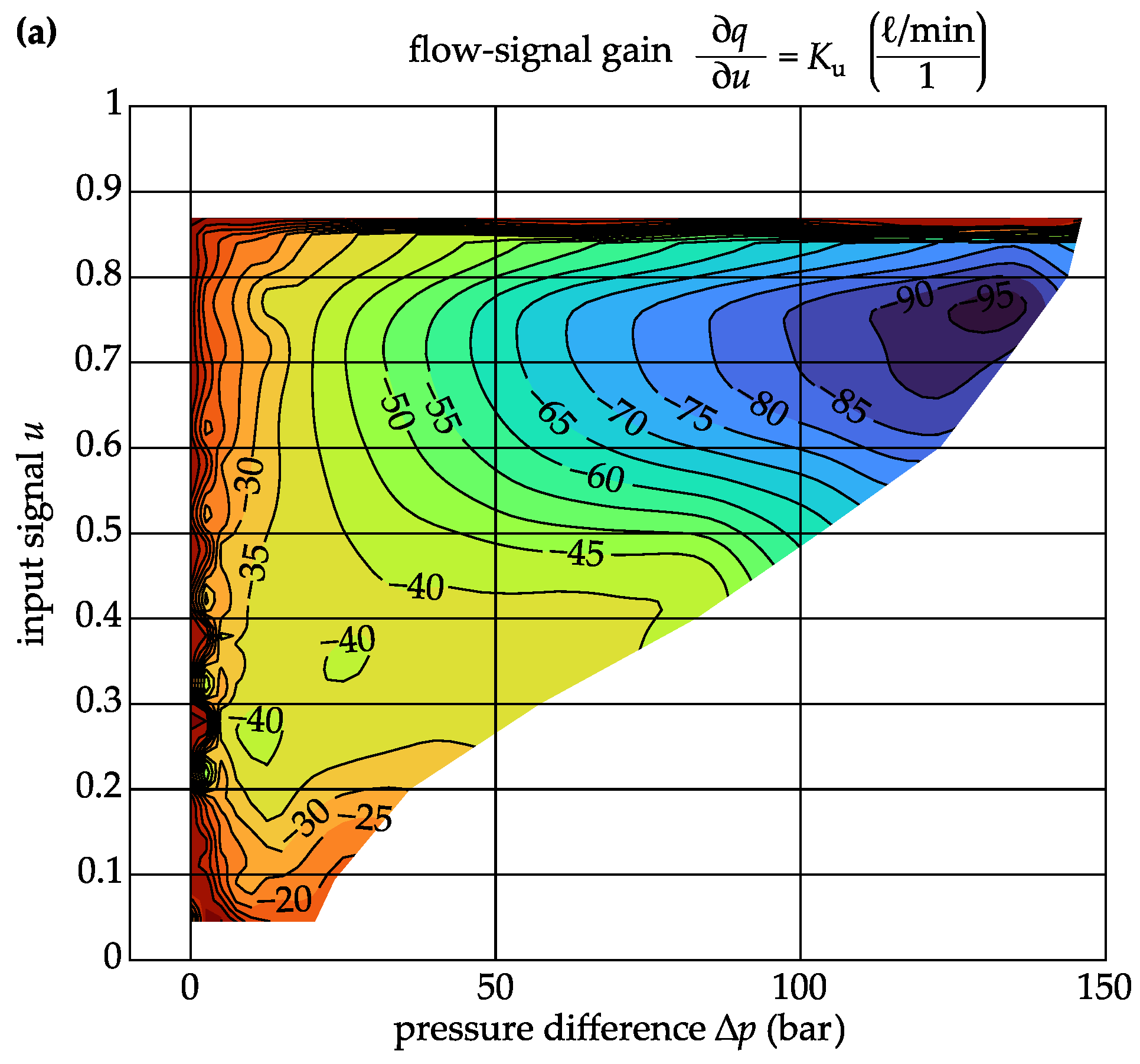
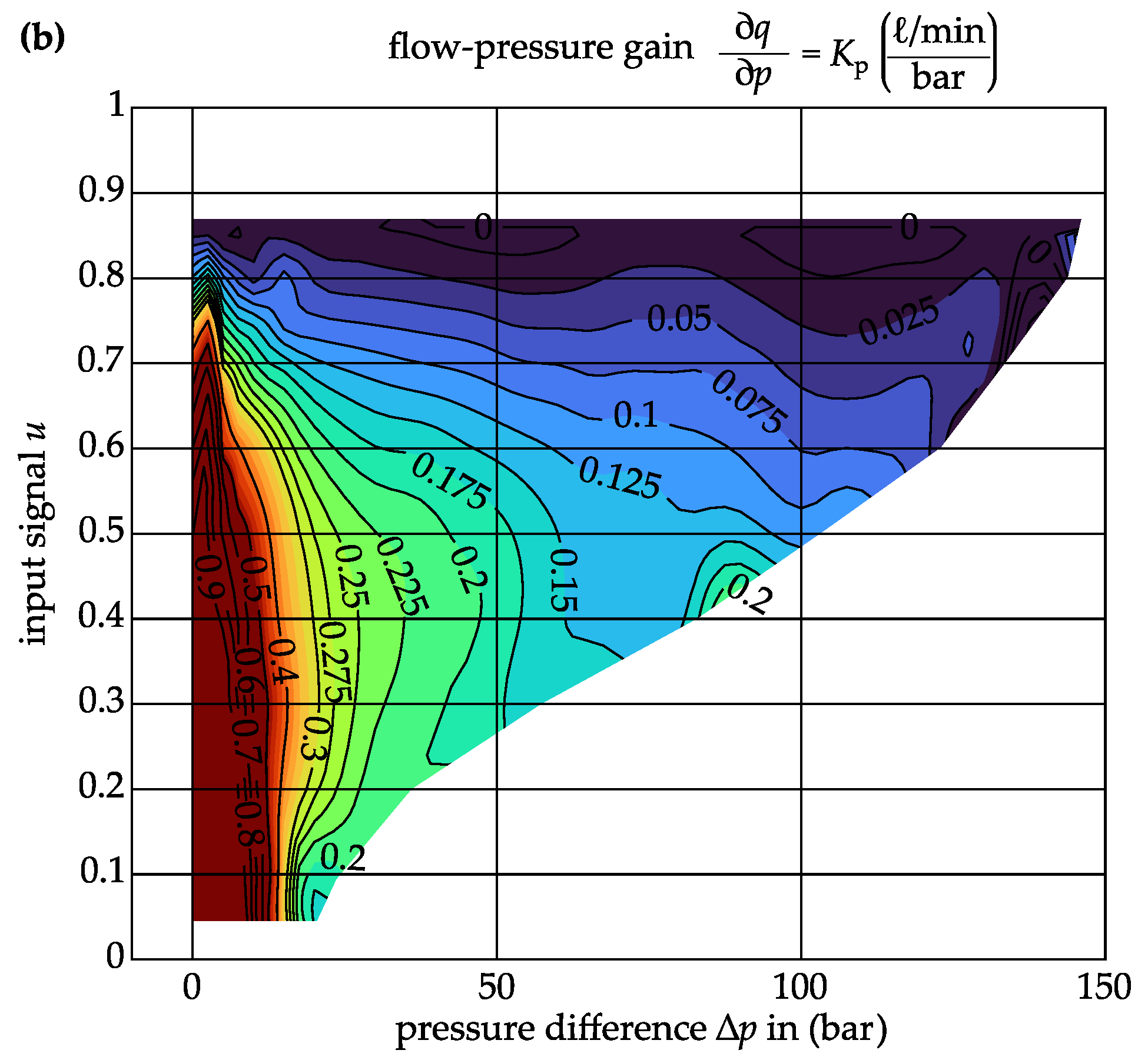
Figure 7.
(a) Lumped parameter model of side A: (b) flow when the pump sucks from the half-bridge, (c) flow when the pump is pumping into the half-bridge.
Figure 7.
(a) Lumped parameter model of side A: (b) flow when the pump sucks from the half-bridge, (c) flow when the pump is pumping into the half-bridge.

Figure 8.
E-BAC control scheme.
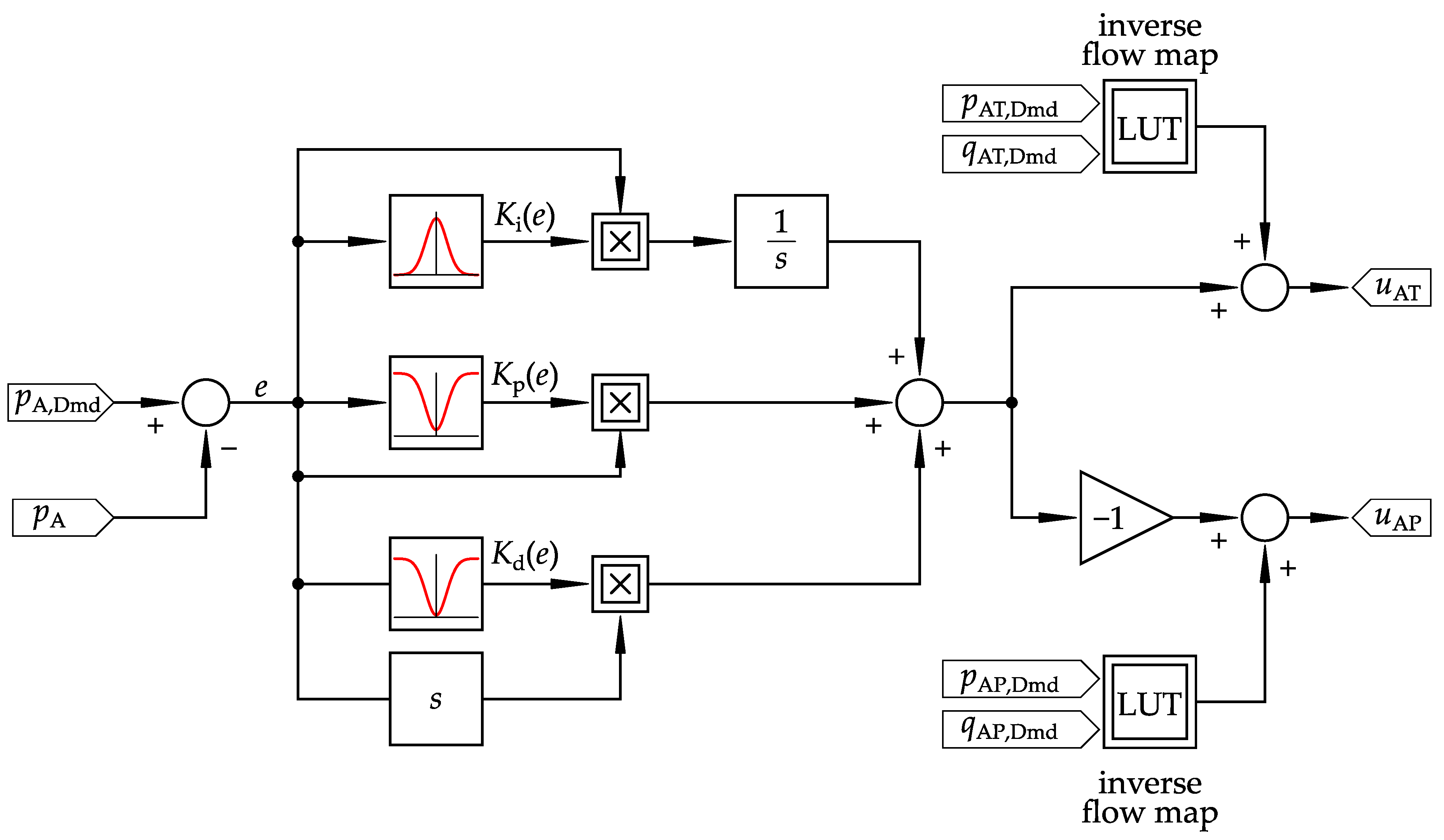
Figure 9.
(a) Error-based proportional gain; (b) error-based integral gain; (c) error-based derivative gain.
Figure 9.
(a) Error-based proportional gain; (b) error-based integral gain; (c) error-based derivative gain.
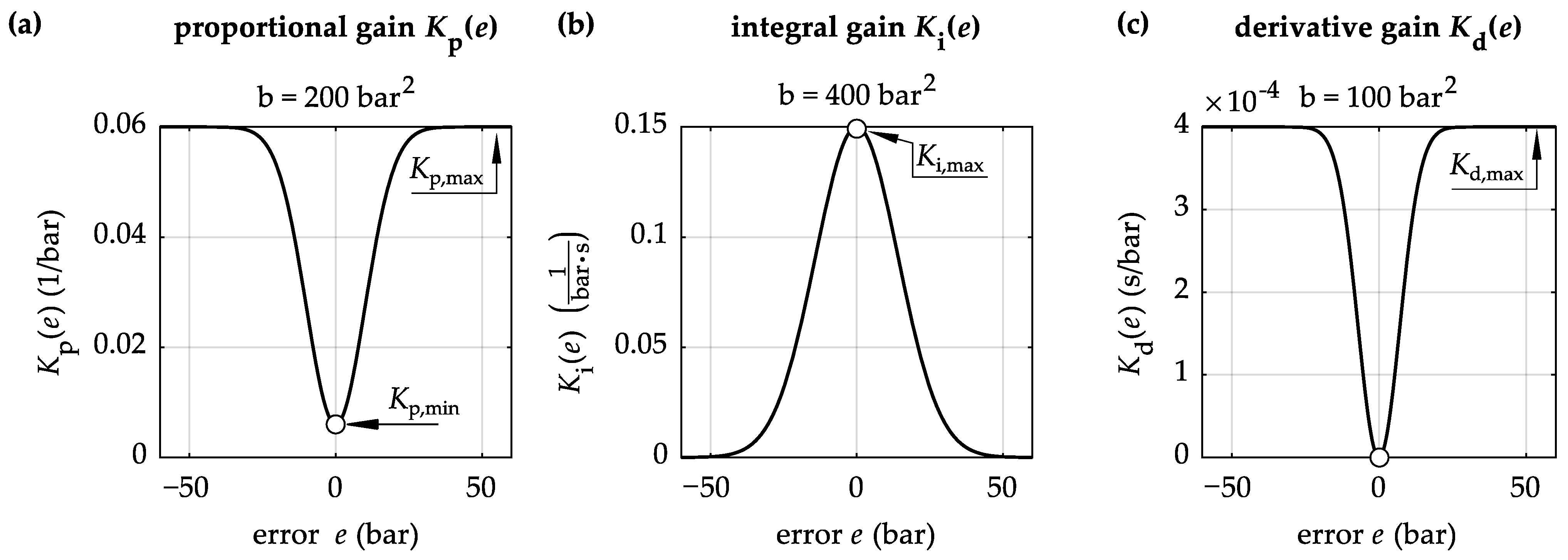
Figure 10.
Pressure step 50 bar with .
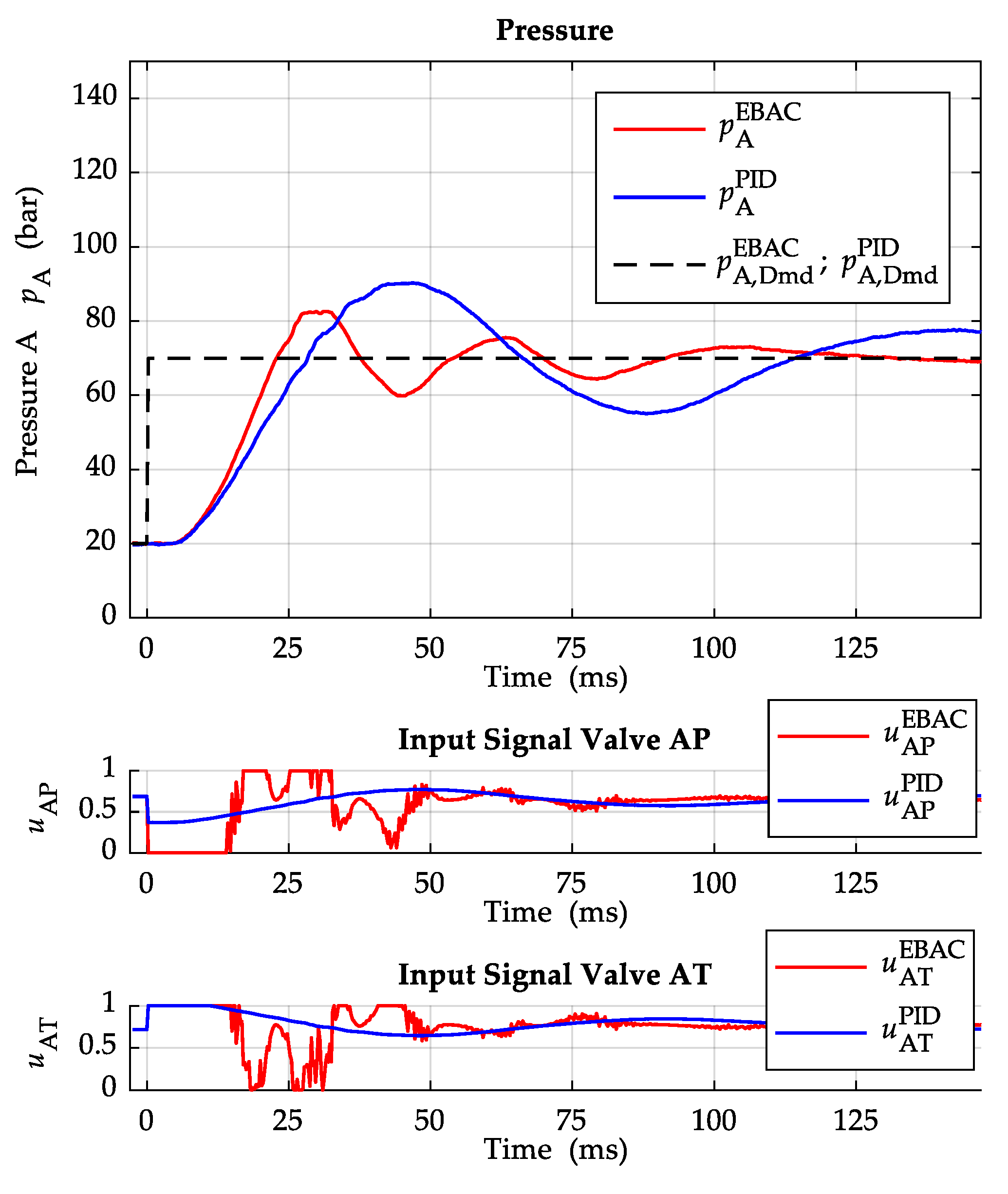
Figure 11.
Pressure step 100 bar with .
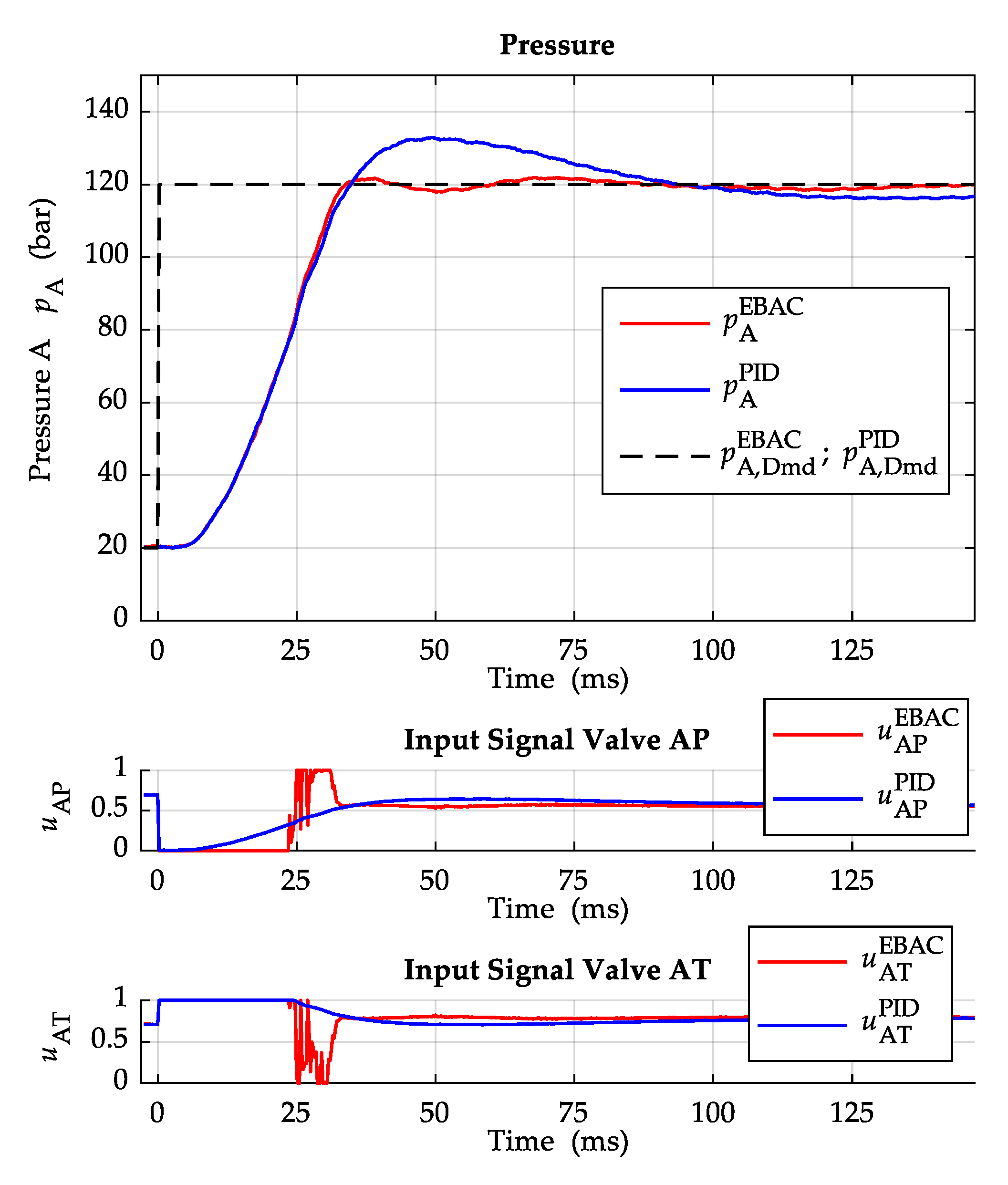
Figure 12.
Pressure step 50 bar with .
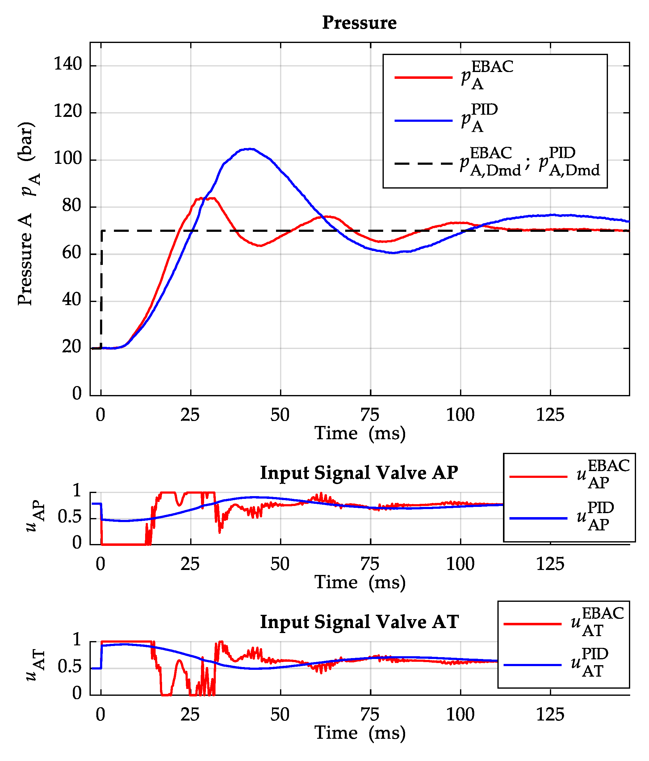
Figure 13.
Pressure step 100 bar with .
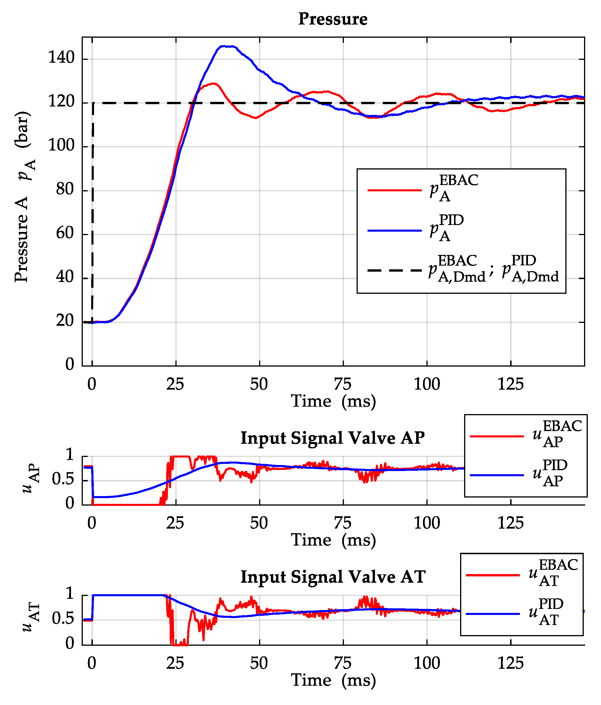
Figure 14.
Fast speed ramp at constant pressure setpoint.
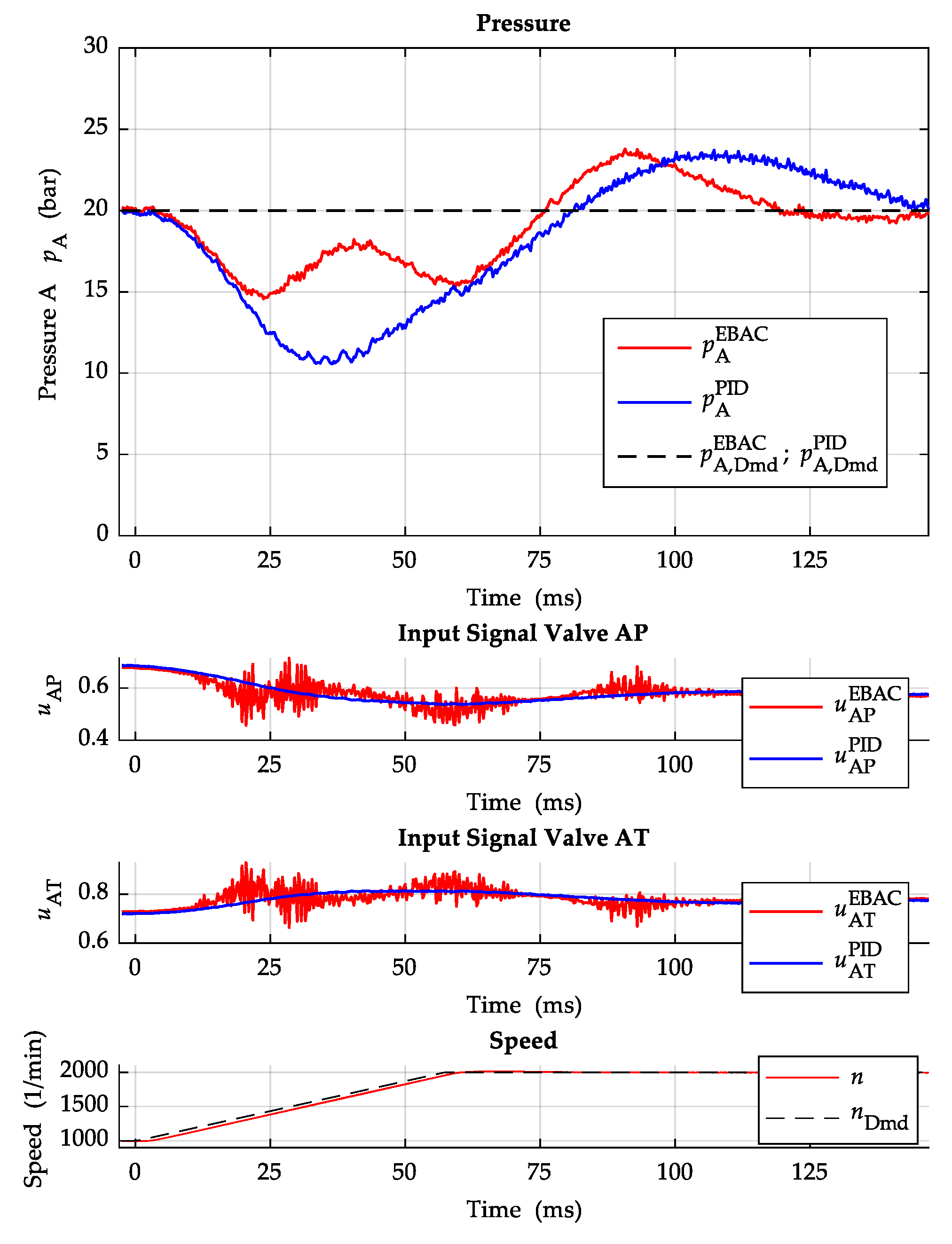
Figure 15.
Test cycle.

Table 1.
Controller gains of E-BAC-Controller for error and for fixed PID-controller.
| Controller | |||
|---|---|---|---|
| E-BAC | |||
| PID | 0.0056 | 0.254 | 0.00003 |
Table 2.
Parameters used for the adaptive error-based gain functions.
| Gain Function | b | ||
|---|---|---|---|
| 0.06 | 0.006 | 200 | |
| 0.15 | — | 400 | |
| 0.0004 | — | 100 |
Disclaimer/Publisher’s Note: The statements, opinions and data contained in all publications are solely those of the individual author(s) and contributor(s) and not of MDPI and/or the editor(s). MDPI and/or the editor(s) disclaim responsibility for any injury to people or property resulting from any ideas, methods, instructions or products referred to in the content. |
© 2023 by the authors. Licensee MDPI, Basel, Switzerland. This article is an open access article distributed under the terms and conditions of the Creative Commons Attribution (CC BY) license (https://creativecommons.org/licenses/by/4.0/).
Share and Cite
MDPI and ACS Style
Pfizenmaier, M.; Pippes, T.; Bohr, A.; Falkenstein, J. Load Emulation with Independent Metering for a Pump Test Bench. Actuators 2023, 12, 413. https://doi.org/10.3390/act12110413
AMA Style
Pfizenmaier M, Pippes T, Bohr A, Falkenstein J. Load Emulation with Independent Metering for a Pump Test Bench. Actuators. 2023; 12(11):413. https://doi.org/10.3390/act12110413
Chicago/Turabian StylePfizenmaier, Max, Thomas Pippes, Artur Bohr, and Jens Falkenstein. 2023. "Load Emulation with Independent Metering for a Pump Test Bench" Actuators 12, no. 11: 413. https://doi.org/10.3390/act12110413
Note that from the first issue of 2016, this journal uses article numbers instead of page numbers. See further details here.