Adaptive PID Controller for Active Suspension Using Radial Basis Function Neural Networks

Abstract

Suspension systems are critical parts of modern cars. In this study, a radial basis function neural networks-based adaptive PID optimal method is presented for vehicle suspension systems. To avoid the shortcoming that the parameters of PID control are determined by experience in the traditional method, to avoid the local optimality problem and the slow rate of convergence in the modern intelligence method, radial basis function neural networks are applied in this paper. First, a quarter-car suspension is presented. Then, the radial basis function neural networks are employed to obtain the parameters of proportional, integral, and derivate components that are used in PID control. The simulation is conducted later. Next, a comparison of the progress between uncontrolled suspension, the radial basis function-based PID control, the $H_{\infty }$ control method, and the FPM control method is presented. According to the simulation results, the proposed control method performs better than the others. This contrast reveals the superior characteristics of the suggested control strategy.

1. Introduction

Vehicle suspension systems have a big impact on how comfortable the ride for passengers is and how well the vehicle holds on the road [1]. Generally speaking, there are three categories of car suspension according to the type of damper and actuator. Passive suspension systems [2] comprise springs and non-adjustable dampers, which make them inadequate for promoting ride quality and steadiness in handling. Semi-active suspension systems [1] are composed of springs and adjustable coefficient dampers. Thus, by modifying the damper, semi-active suspension systems can provide passengers with greater comfort. In contrast to the other two types of suspension systems, there are active actuators equipped with active vehicle suspensions [3]. At the same time, the actuator can create the necessary force by assimilating or liberating load to minimize vibration. Therrefore, this type of suspension can dramatically improve vehicle performance as a result [4].

To deal with the challenging issue of increasing vehicle performance, numerous control strategies have been developed and used for the vehicle control program [5,6,7,8,9,10].

For example, [5] developed a reliable control method that combines sliding mode control and LQR optimal control for an uncertain car suspension system. In [6], an intelligent nonlinear controller that combines SMC, fuzzy logic, and neural network techniques was presented. In study [7], an SMC-based adaptive control method was developed. AA Basari et al. proposed a nonlinear controller for quarter-car suspension using a backstepping control approach [8]. In study [9], an adaptive backstepping control algorithm was presented to make the vehicle more comfortable and stable in the face of parameter uncertainty. In [10], a robust $H\infty$ control with LMI optimization for active suspension control under non-stationary conditions was investigated.

PID control is currently utilized with increasing frequency in closed-loop control systems because it is an effective, simple, highly dependable, and simple-to-use control technology [11], and it has been widely used in vehicle systems [12,13,14]. A PID controller was designed for active suspension systems [12]. In the literature [13], a stochastically optimized PID controller for a linear two-DOF suspension model has been discussed. An adaptive fuzzy PID controller was presented to improve the performance of vehicles based on road evaluations [14]. PID control has a very broad range of applications, and for various control objects, the controller’s performance criteria are often highly varied.

However, there are still some issues with PID control in practice. One of the most difficult problems is the parameterization of the PID because it is difficult to alter the proportional integral and derivative components to produce the best outcome.

In the research conducted on PID control, ample methods have been presented to optimize the parameters used in PID. Generally speaking, there are three traditional and common methods of PID regulation: manual adjustment, traditional parameter optimization methods, and model-based methods.

Nevertheless, the manual adjustment method and traditional method are time-consuming, imprecise, and often difficult. Model-based methods need to be built on an accurate physical model; it is challenging to obtain optimal performance for systems with uncertain characteristics when using set PID parameters, which cannot be changed to reflect changes in the system.

In [15], a fuzzy controller that uses the PID-based method for active suspension was investigated. In [16], a PID-based control method was applied to the active suspension systems. Iterative learning was used in this controller architecture to adjust PID gains. In study [17], a novel method was used to obtain PID parameters for active actuators. These methods are able to substantially improve the performance of the closed-loop system compared with the conventional methods. However, the disadvantages of these methods are also obvious. The learning ability is poor, and the optimization search process is long and time-consuming.

With the development of computer technology, artificial intelligence methods combined with PID control have received widespread attention. PSO is used in fuzzy-based PID control for half-vehicle suspension models [18]. The authors of [19] used a genetic algorithm to optimize PID and LQR control and employed these optimization controllers for suspension systems. In [20], the artificial fish swarm algorithm was used in the optimization of a PID controller. These artificial intelligence-based methods can shorten the time of optimization seeking but are prone to experiencing local optimization problems.

To significantly speed up learning and avoid the local minimum problem, a new approach is required. Radial basis function neural networks are feedforward networks and are constituted by three layers: input, hidden, and output. The third layer is also constituted by linear neurons. It is possible to map the first layer node to the third layer node [21]. And the mapping is nonlinear, so it could be employed in selecting optimal parameters. This makes it possible to accelerate the adjustment of the PID parameters and improve their robustness and anti-interference. Using this method can also reduce the optimization time while avoiding the local optimization problem. As a result, it is possible to calculate the objective function for whole neural networks, and the rate of learning is lower.

Thus, in this paper, the radial basis function neural networks approach is used to overcome the shortcoming that the parameters of PID control are determined by experience in the traditional active suspension control. The radial basis function neural networks approach is also used to speed up learning and avoid the local minimum problem in suspension control. Therefore, the radial basis function neural networks-based adaptive PID control method is used for active suspension control.

The structure of this research is presented as follows. In the second section, a quarter-car suspension model is carried out. In the third section, the radial basis function neural networks-based adaptive PID optimal control strategy is presented. Alongside this, the stability proof of the proposed closed-loop systems is presented. In the fourth section, the simulation results and discussion are shown. In addition, in order to verify the performance of the proposed controller, a comparison is discussed between the proposed control method, the FPM method [14] and $H_{\infty }$ [22]. In the final section, conclusions are drawn and recommendations are made.

2. System Model

2.1. Road Profile

To demonstrate the effectiveness of the proposed control technique, the system models should be presented at first. Typically, the employed inputs include random inputs, the step response, the bump road, and the sine function. The sine function is used as an input in this research. The continuous sine road profile is given as follows:

$$x_g=sin(4\times t)$$

(1)

2.2. Suspension Model

As the performance of the quarter-car system model is straightforward as well as effective at capturing the key component elements, a two-DOF suspension model is used in this research and is shown in Figure 1. The quarter model includes the key basic properties: sprung mass acceleration and displacement, suspension deflection, and tire deflection.

The parameter descriptions in Figure 1 are illustrated as follows:

• $m_s$: car body mass;
• $m_u$: unsprung mass;
• $k_s$: suspension stiffness;
• $k_t$: stiffness of tire;
• u: force produced by the actuator;
• $c_s$:coefficient of damper;
• $x_g$, $x_u$, and $x_s$ indicate the road profile and the displacement of the unsprung and sprung masses, respectively.

The dynamic functions of quarter-car suspension systems are shown as follows:

$$\ddot{x_s}=\frac{u}{m_s}-\frac{k_s}{m_s}(x_s-x_u)-\frac{c_s}{m_s}(\dot{x_s}-\dot{x_u})$$

(2)

$$\ddot{x_u}=-\frac{u}{m_u}+\frac{k_t}{m_u}(x_g-x_u)+\frac{k_s}{m_u}(x_s-x_u)+\frac{c_s}{m_u}(\dot{x_s}-\dot{x_u})$$

(3)

The following definitions are the state variables. The state variables have been proven to aid in control synthesis and establish the output matrix and state matrix.

$$X={\left[\begin{array}{cccc}{x}_s-x_u& \dot{x_s}& x_g-x_u& \dot{x_u}\end{array}\right]}^T$$

$$Y={\left[\begin{array}{cccc}\ddot{x_s}& x_s-x_u& x_g-x_u& u\end{array}\right]}^T$$

where

• ${\ddot{x}}_s$ is the sprung mass acceleration;
• $x_s-x_u$ is the suspension deflection;
• $x_g-x_u$ depicts the dynamic deflection of the tire;
• u symbolizes the force that is conducted by the actuator.

As a result, the state space notation representing the dynamic differential function for active suspension is shown as follows:

$$\dot{X}=AX+BU+FW$$

(4)

$$Y=CX+DU$$

(5)

where

$$A=\left[\begin{array}{cccc}0& 1& 0& -1\\ -\frac{k_s}{m_s}& -\frac{c_s}{m_s}& 0& \frac{c_s}{m_s}\\ 0& 0& 0& -1\\ \frac{k_s}{m_u}& \frac{c_s}{m_u}& \frac{k_t}{m_u}& -\frac{c_s}{m_u}\end{array}\right],$$

$$B=\left[\begin{array}{c}0\\ 1/m_s\\ 0\\ -1/m_u\end{array}\right],$$

$$C=\left[\begin{array}{cccc}-k_s/m_s& 0& 0& 0\\ 1& 0& 0& 0\\ 0& 0& k_t& 0\\ 0& 0& 0& 0\end{array}\right],$$

$$F=\left[\begin{array}{c}0\\ 0\\ 1\\ 0\end{array}\right],$$

$$D=\left[\begin{array}{c}\frac{1}{m_s}\\ 0\\ 0\\ 1\end{array}\right],$$

$$U=\left[u\right],W=\left[{\dot{x}}_g\right].$$

3. Controller Design

In this section, the RBF-based adaptive PID control method is discussed. Moreover, the $H_{\infty }$ control method and FPM method [14] are also offered to improve the performance of active suspension systems.

3.1. PID Control

PID control consists of a continuous form and discrete form. PID control algorithms are generally operated in computer systems using numerical approximation. Computer operations are discrete. Therefore, in order to enable the computer to implement the PID algorithm program, it is necessary to discretize the continuous functions of the PID algorithm.

The following approximate process can be obtained when the sampling period is small enough:

$$\begin{array}{cc}\hfill u\left(t\right)& \simeq u\left(k\right)\hfill \end{array}$$

(6)

$$\begin{array}{cc}\hfill e\left(t\right)& \simeq e\left(k\right)\hfill \end{array}$$

(7)

$${\int }_0^{t}e\left(t\right)dt=\sum _{i=0}^{k}e\left(i\right)\mathsf{\Delta }t=\sum _{i=0}^{k}Te\left(i\right)$$

(8)

$$\frac{de\left(t\right)}{dt}\simeq \frac{e\left(k\right)-e(k-1)}{\mathsf{\Delta }t}=\frac{e\left(k\right)-e(k-1)}{T}$$

(9)

where T is the sampling period. k is the sampling serial number.

Using this approximation, two PID control methods can be obtained: positional and incremental. In this paper, the incremental PID control method is discussed; Figure 2 illustrates the structure of the incremental PID control method.

PID controllers are composed of pieces that are proportional, integral, and derivative [11], where:

• $y\left(k\right)$: the actual response;
• $r\left(k\right)$: the desired response;
• $k_p$: the proportional gain;
• $k_i$: the integral gain;
• $k_d$: the derivate gain.

$e\left(k\right)$ is the error produced in the control, which has the following expressions:

$$e\left(k\right)=r\left(k\right)-y\left(k\right)$$

(10)

The inputs are represented as follows:

$$\left\{\begin{array}{c}{x}_c\left(1\right)=e\left(k\right)-e(k-1)\hfill \\ x_c\left(2\right)=e\left(k\right)\hfill \\ x_c\left(3\right)=e\left(k\right)-2e(k-1)+e(k-2)\hfill \end{array}\right.$$

(11)

The control algorithm is shown as follows:

$$u\left(k\right)=u(k-1)+\mathsf{\Delta }u\left(k\right)$$

(12)

$$\begin{array}{cc}\hfill \mathsf{\Delta }u\left(k\right)& =k_p\left(e\left(k\right)-e\left(k-1\right)\right)+k_{i}e\left(k\right)+k_d\left(e\left(k\right)-2e\left(k-1\right)+\left(k-2\right)\right)\hfill \\ & =k_p{x}_c\left(1\right)+k_i{x}_c\left(2\right)+k_d{x}_c\left(3\right)\hfill \end{array}$$

(13)

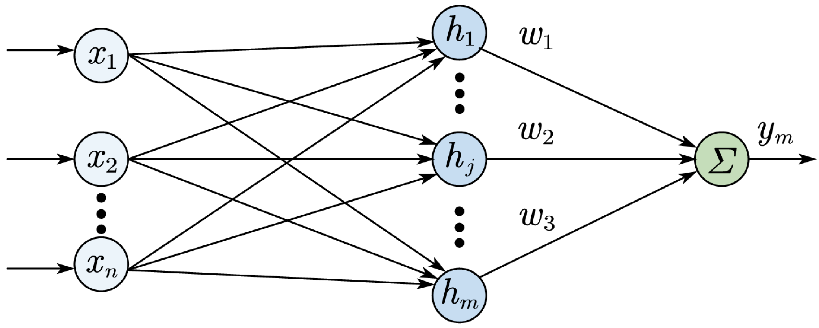
3.2. Radial Basis Function Neural Networks (RBF-NNs)

Radial basis function neural networks model the regional changes in the human brain and encompass receptive fields. It has been demonstrated that this method can approach any function with freewill precision [21].

In Figure 3, the structure of radial basis function neural networks is presented.

The input of neural networks is presented.

$$X={\left[\begin{array}{cccc}{x}_1& x_2& \cdots & x_n\end{array}\right]}^T$$

The vector of the radial basis is provided as H.

$$H={\left[\begin{array}{cccccc}{h}_1& h_2& \cdots & h_j& \cdots & h_m\end{array}\right]}^T$$

The following is the expression of the Gauss basis function.

$$h_j=exp\left(-\frac{\left||X-c_j\right||}{2{b_j}^2}\right)$$

(14)

The basis width vector is shown as follows.

$$B={\left[\begin{array}{cccc}{b}_1& b_2& \cdots & b_m\end{array}\right]}^T$$

(15)

The radial basis function neural networks weight vector is displayed as follows.

$$W={\left[\begin{array}{cccccc}{w}_1& w_2& \cdots & w_j& \cdots & w_m\end{array}\right]}^T$$

(16)

In light of this, the radial basis function neural networks output is displayed as follows.

$$y_m\left(k\right)=w_1{h}_1+w_2{h}_2+\cdots +w_m{h}_m$$

(17)

3.3. Hybrid Controller

The closed-loop system is composed of suspension systems and a controller. The controller consists of two components: (1) a conventional PID controller that provides direct closed-loop control of the suspension system, and the three parameters $k_p$, $k_i$, and $k_d$ can be tuned online or offline; and (2) the radial basis function neural networks, which regulate the PID parameters according to the operating state of the system to achieve optimal system performance. That is, the output states of the neurons in the output layer correspond to the three parameters of the PID. Through the radial basis function neural networks’s learning, the weighting coefficients are adjusted so as to optimize the system’s performance.

The radial basis function neural networks rectification purpose is represented as follows.

$$E\left(k\right)=\frac{1}{2}e{\left(k\right)}^2$$

(18)

The input of RBF-NNs are $r\left(k\right)$, the desired output; $y\left(k\right)$, the actual output; and $e\left(k\right)$, the error.

The detailed design process of the controller is as follows.

• Step 1
  Determine the structure of the neural network, the number of the node in the input layer, the hidden layer, and the output layer. Choose the learning rate $\eta$ and the initial value of weighting coefficient W. $k=1$.

• Step 2
  $r\left(k\right)$, $y\left(k\right)$ can be obtained by sampling. Calculate the error $e\left(k\right)$. In this paper, the acceleration of body mass suspension is chosen as $y\left(k\right)$. The desired output is $r\left(k\right)=0$.

• Step 3
  Calculate the inputs and outputs of each neural node. Calculate the output of each layer.
  $W^1$ is the output weighting matrix from the input layer to the hidden layer. ${w_{nj}}^1$ is the weighting coefficient from $n^{th}$ code of the input layer to $j^{th}$ code of the hidden layer. $W^2$ is the output weighting matrix from the hidden layer to the output layer. $W^1$ and $W^2$ are presented as follows. $W^1$ is the given weight matrix.

  $$W^1=\left|\begin{array}{ccc}{w_{11}}^1& {w_{12}}^1& {w_{13}}^1\\ {w_{21}}^1& {w_{22}}^1& {w_{23}}^1\\ {w_{31}}^1& {w_{32}}^1& {w_{33}}^1\end{array}\right|$$
  The weighting coefficients in $W^2$ are calculated as follows.

  $${w_j}^2\left(k\right)={w_j}^2(k-1)+\eta \left(k\right)e\left(k\right)h_j+\beta \left({w_j}^2(k-1)-{w_j}^2(k-2)\right)$$

  (19)

  where $\mathbf{h}={\left[h_j\right]}^T$ is the output of the hidden layer. $h_j$ is the output of $j^{th}$ code in the hidden layer. $\eta \left(k\right)$ is the scaling factor when updating the weights of the RBF-based PID control.
  $\eta \left(k\right)$ can be calculated online by the following equation [23].

  $$\eta \left(k\right)=\left\{\begin{array}{c}5{\eta }_0\left(1-logsigmoid\left(-e{\left(k\right)}^2\right)\right),e\left(k\right)\ge 0.368\times e_0\hfill \\ {\eta }_0,e\left(k\right)<0.368\times e_0\hfill \end{array}\right.$$

  (20)

  where $e_0=r\left(k\right)-y_0\left(k\right)$; ${\eta }_0$ is not randomly selected and can be obtained from the stability of the proof.
  The central node $c_j\left(k\right)$ can be calculated as follows.

  $$c_j\left(k\right)=c_j(k-1)+\eta \mathsf{\Delta }{c}_j\left(k\right)+\beta \left(c_j(k-1)-c_j(k-2)\right)$$

  (21)

  where $\mathsf{\Delta }{c}_j\left(k\right)=e\left(k\right){w_j}^2\left(k\right)\frac{x_i-c_j}{{b_j}^2}$.
  The base width of node $b_j$ can be calculated as follows.

  $$\begin{array}{cc}\hfill b_j\left(k\right)& =b_j(k-1)+\eta \left(k\right)\mathsf{\Delta }{b}_j+\beta \left(b_j(k-1)-b_j(k-2)\right)\hfill \end{array}$$

  (22)

  $$\begin{array}{cc}\hfill \mathsf{\Delta }{b}_j& =\left(y\left(k\right)-y(k-1)\right){w_j}^2\left(k\right)\frac{{∥X-C_j∥}^2}{{b_j}^3}\hfill \end{array}$$

  (23)
  In this research, the gradient descent method is utilized [24] to obtain the updating rules.

  $$\frac{\partial E\left(k\right)}{\partial {W_j}^2\left(k\right)}=\frac{\partial E\left(k\right)}{\partial e\left(k\right)}\frac{\partial e\left(k\right)}{\partial y\left(k\right)}\frac{\partial y\left(k\right)}{\partial u\left(k\right)}\frac{\partial u\left(k\right)}{\partial {W_j}^2\left(k\right)}=-e\left(k\right)\frac{\partial y\left(k\right)}{\partial u\left(k\right)}{a}_j\left(k\right)\eta \left(k\right)$$

  (24)

  where $\partial y\left(k\right)/\partial u\left(k\right)$ can be replaced by $sgn\left(\partial y\left(k\right)/\partial u\left(k\right)\right)$.
  Then, the weight matrix can be obtained as follows.

  $$\mathsf{\Delta }\partial {W_j}^2\left(k\right)\left(k\right)=\frac{\partial E\left(k\right)}{\partial {W_j}^2\left(k\right)\left(k\right)}=\eta \left(k\right)e\left(k\right)sgn\left(\frac{\partial y\left(k\right)}{\partial u\left(k\right)}\right)a_j\left(k\right)$$

  (25)
  So, the adjustment volume of $k_p$, $k_i$, and $k_d$ are shown as follows.

  $$\begin{array}{c}\hfill \mathsf{\Delta }{k}_p=\eta \left(k\right)e\left(k\right)\frac{\partial y\left(k\right)}{\partial u}{x}_c\left(1\right)\end{array}$$

  (26)

  $$\begin{array}{c}\hfill \mathsf{\Delta }{k}_i=\eta \left(k\right)e\left(k\right)\frac{\partial y\left(k\right)}{\partial u}{x}_c\left(2\right)\end{array}$$

  (27)

  $$\begin{array}{c}\hfill \mathsf{\Delta }{k}_d=\eta \left(k\right)e\left(k\right)\frac{\partial y\left(k\right)}{\partial u}{x}_c\left(3\right)\end{array}$$

  (28)

  where $\frac{\partial y\left(k\right)}{\partial u}$ is the Jacobin value of the control objective. $\frac{\partial y\left(k\right)}{\partial u}$ can be calculated by the following equation.

  $$\frac{\partial y\left(k\right)}{\partial u}=\sum _{j=1}^3{w_j}^2\left(k\right)h_j\frac{c_j-x_1}{2{b_j}^2}$$

  (29)

• $\mathbf{Step}\mathbf{4}$
  Calculate $u\left(k\right)$.

  $$u\left(k\right)=u(k-1)+\mathsf{\Delta }u\left(k\right)$$

  (30)
  $\mathsf{\Delta }u\left(k\right)$ can be obtained by the following.

  $$\begin{array}{cc}\hfill \mathsf{\Delta }u\left(k\right)& =k_p\left(e\left(k\right)-e\left(k-1\right)\right)+k_{i}e\left(k\right)+k_d\left(e\left(k\right)-2e\left(k-1\right)+\left(k-2\right)\right)\hfill \\ & =k_p{x}_c\left(1\right)+k_i{x}_c\left(2\right)+k_d{x}_c\left(3\right)\hfill \end{array}$$

  (31)
  $k_p\left(k\right),k_i\left(k\right),k_d\left(k\right)$ are calculated by the following equations.

  $$\begin{array}{cc}\hfill k_p\left(k\right)& =k_p\left(1\right)+\mathsf{\Delta }{k}_p\hfill \end{array}$$

  (32)

  $$\begin{array}{cc}\hfill k_i\left(k\right)& =k_i\left(1\right)+\mathsf{\Delta }{k}_i\hfill \end{array}$$

  (33)

  $$\begin{array}{cc}\hfill k_d\left(k\right)& =k_d\left(1\right)+\mathsf{\Delta }{k}_d\hfill \end{array}$$

  (34)

  where $k_p\left(1\right)$, $k_i\left(1\right)$, and $k_d\left(1\right)$ are the initial value and given values.

• $\mathbf{Step}\mathbf{5}$
  Calculate $y\left(k\right)$ and $E\left(k\right)$.

• $\mathbf{Step}\mathbf{6}$
  Determine whether $E\left(k\right)$ satisfies the requirement. If satisfied, output $k_p,k_i,k_d$; otherwise, return to Step 1, $k=k+1$.

The flowchart of the proposed hybrid control is shown in Figure 4.

3.4. Stability Analysis of the Controller

The following illustrates the stability analysis of the suspension closed system.

Theorem 1. 

At any k sample steps, if the scaling factor $\eta \left(k\right)$ meets the following conditions,

$$\left|\eta \left(k\right)\right|<\sqrt{2{\left(\sum _{j=1}^3{a_j}^2\left(k\right)\right)}^{-1}}$$

(35)

Then, the closed-loop system is stable.

Proof of Theorem 1. 

To demonstrate the stability of the closed-loop system with the suggested controller, the Lyapunov stability theory is used and is now defined as follows. □

$$V\left(k\right)=\frac{1}{2}e{\left(k\right)}^2,e\left(k\right)=r\left(k\right)-y\left(k\right)$$

(36)

where $r\left(k\right)$ is the desired reference signal and $y\left(k\right)$ is the actual output signal. $a_j\left(k\right)$ is the output of the hidden layer.

$$\begin{array}{c}\mathsf{\Delta }V\left(k\right)=V(k+1)-V\left(k\right)\\ =\frac{1}{2}(e{(k+1)}^2-e{\left(k\right)}^2)\end{array}$$

(37)

when

$$\mathsf{\Delta }e\left(k\right)=\sum _{j=1}^3\frac{\partial e\left(k\right)}{\partial W_{2j}\left(k\right)}\mathsf{\Delta }{W}_{2j}\left(k\right)$$

(38)

then

$$\frac{\partial e\left(k\right)}{\partial W_{2j}\left(k\right)}=\frac{\partial e\left(k\right)}{\partial y\left(k\right)}\frac{\partial y\left(k\right)}{\partial u\left(k\right)}\frac{\partial u\left(k\right)}{\partial W_j\left(k\right)}$$

(39)

$$=-sgn\left(\frac{\partial y\left(k\right)}{\partial u\left(k\right)}\right)\eta \left(k\right)a_j\left(k\right)$$

Next,

$$\mathsf{\Delta }e\left(k\right)=-\sum _{j=1}^3\left(\frac{\partial y\left(k\right)}{\partial u\left(k\right)}\right)\eta \left(k\right)a_j\left(k\right)\times \eta \left(k\right)e\left(k\right)sgn\left(\frac{\partial y\left(k\right)}{\partial u\left(k\right)}\right)a_j\left(k\right)$$

(40)

$$=-\sum _{j=1}^3{\left(sgn\left(\frac{\partial y\left(k\right)}{\partial u\left(k\right)}\right)\right)}^2\eta {\left(k\right)}^2{a_j}^2\left(k\right)e\left(k\right)$$

since

$${\left(sgn\left(\frac{\partial y\left(k\right)}{\partial u\left(k\right)}\right)\right)}^2=1$$

(41)

then

$$\mathsf{\Delta }e\left(k\right)=-\sum _{j=1}^3{\left(\eta \left(k\right)\right)}^2{a_j}^2\left(k\right)e\left(k\right)$$

(42)

as

$$e(k+1)=e\left(k\right)+\mathsf{\Delta }e\left(k\right)$$

(43)

then

$$\mathsf{\Delta }V\left(k\right)=\frac{1}{2}(e(k+1)-e\left(k\right))(e(k+1)+e\left(k\right))$$

(44)

$$=\frac{1}{2}\mathsf{\Delta }e\left(k\right)(\mathsf{\Delta }e\left(k\right)+2e\left(k\right))$$

$$=e\left(k\right)\mathsf{\Delta }e\left(k\right)+\frac{1}{2}\mathsf{\Delta }e{\left(k\right)}^2$$

The closed-loop system is stable when $\mathsf{\Delta }V\left(k\right)\to 0$ in any sampling period k, depending on the Lyapunov stability theory.

$$e\left(k\right)\mathsf{\Delta }e\left(k\right)<-\frac{\mathsf{\Delta }}{e}{\left(k\right)}^2$$

(45)

then

$$-e\left(k\right)\sum _{j=1}^3{\left(\eta \left(k\right)\right)}^2{a_j}^2\left(k\right)e\left(k\right)<-\frac{1}{2}{\left(-\sum _{j=1}^3{\left(\eta \left(k\right)\right)}^2{a_j}^2\left(k\right)e\left(k\right)\right)}^2$$

(46)

thus

$$2{\left(\sum _{j=1}^3{a_j}^2\left(k\right)\right)}^{-1}>{\left(\eta \left(k\right)\right)}^2$$

(47)

The stability of the closed-loop control system using the suggested PID controller can be assured based on the Lyapunov stability theory, $\mathsf{\Delta }V\left(k\right)<0$, for every sampling step k. Due to the monotonic declining nature of the Lyapunov function $V\left(k\right)$ and the fact that its lower limit is 0, both $V(k+1)=V\left(k\right)=0$ and $\mathsf{\Delta }V\left(k\right)=0$ are true when $k\to \infty$. Because $\eta \left(k\right)$ meets the stability condition, it may be inferred that this is a necessary condition for $\mathsf{\Delta }V\left(k\right)\le 0$.

4. Results and Discussion

To verify the excellence of the proposed control method, two other methods are discussed in this paper. A method is discussed in [14], and another is discussed in [22]. These methods are used for active suspension. A comparison is presented among these methods. The method discussed in [14] uses the fuzzy PID (FPM) algorithm to improve the various performances for active suspension. The method discussed ($H_{\infty }$) [22] is also applied for active suspension.

The RMS value visualizes the degree of vibration. In this research, the RMS value is used to appraise how well the controller performs for active suspension. The root mean square (RMS) is the effective value, which is the square root of the average of the squares of a set of statistics. The calculation process of RMS is expressed as follows.

$$X_{rms}=\sqrt{\frac{{\displaystyle \sum _N^{i=1}}{X_i}^2}{N}}=\sqrt{\frac{{X_1}^2+{X_2}^2+\cdots +{X_N}^2}{N}}$$

(48)

where $X_i$ is the amplitude of the collected signal at a certain point in time. N is the number of signal samples collected.

Three methods are applied in the simulation after the controller model discussed in this study. The first method applies the $H_{\infty }$ algorithm to improve the performance of suspension. The second method applies the radial basis function neural networks to obtain the parameters. The third method is the FPM control method. A comparison is discussed between these methods. A two-DOF car model is applied to confirm the effectiveness of the proposed control strategy, and the parameters used in this model are presented in

Table 1. Quarter-car model parameters.

Parameter	Meaning	Value
$m_s$	Sprung mass	350 kg
$m_u$	Unsprung mass	50 kg
$k_s$	Suspension stiffness	180 N/m
$k_t$	Tire stiffness	190 kN/m
$c_s$	Damper coefficient	1 kN·s/m

.

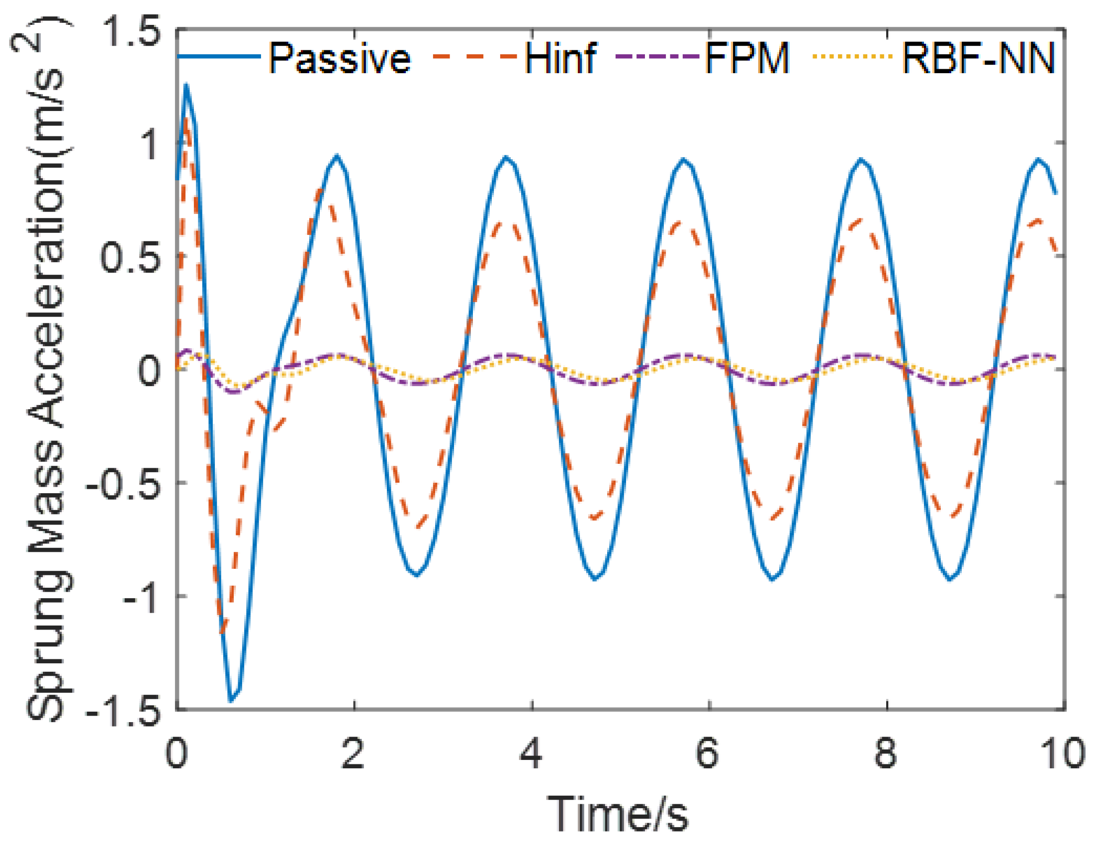
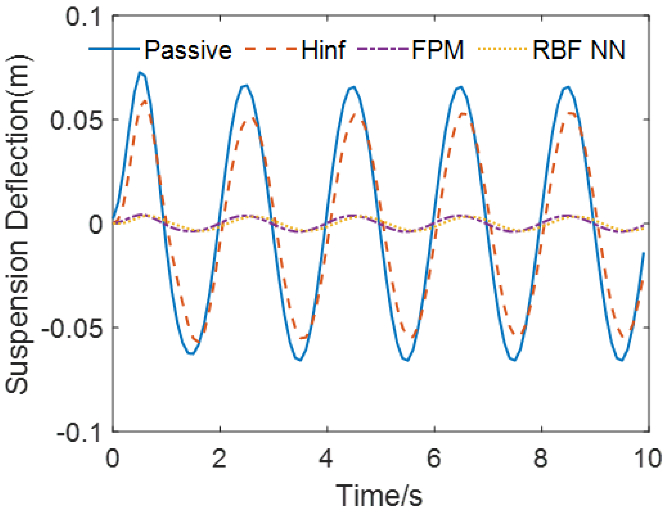
The application of the recommended control technique is used to evaluate the main parts of the system. The sprung mass acceleration, deflection of the suspension and tire, and force produced by the actuator are chosen as evaluation metrics in this paper.

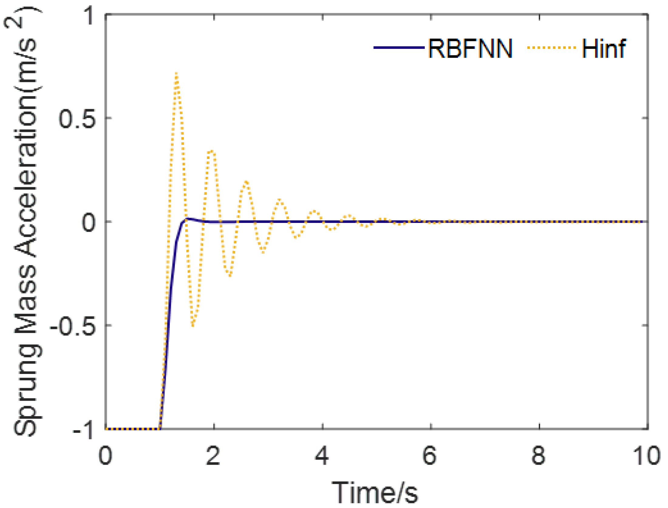
While vehicle body acceleration and suspension deflection have lower values, passenger comfort has a higher performance. Tire deflection is less desirable compared with road-holding performance. The outcomes of the simulation are now displayed to emphasize the salient features of the suggested control method. The simulation findings for the evaluation metrics are shown in Figure 5, Figure 6, Figure 7, Figure 8 and Figure 9.

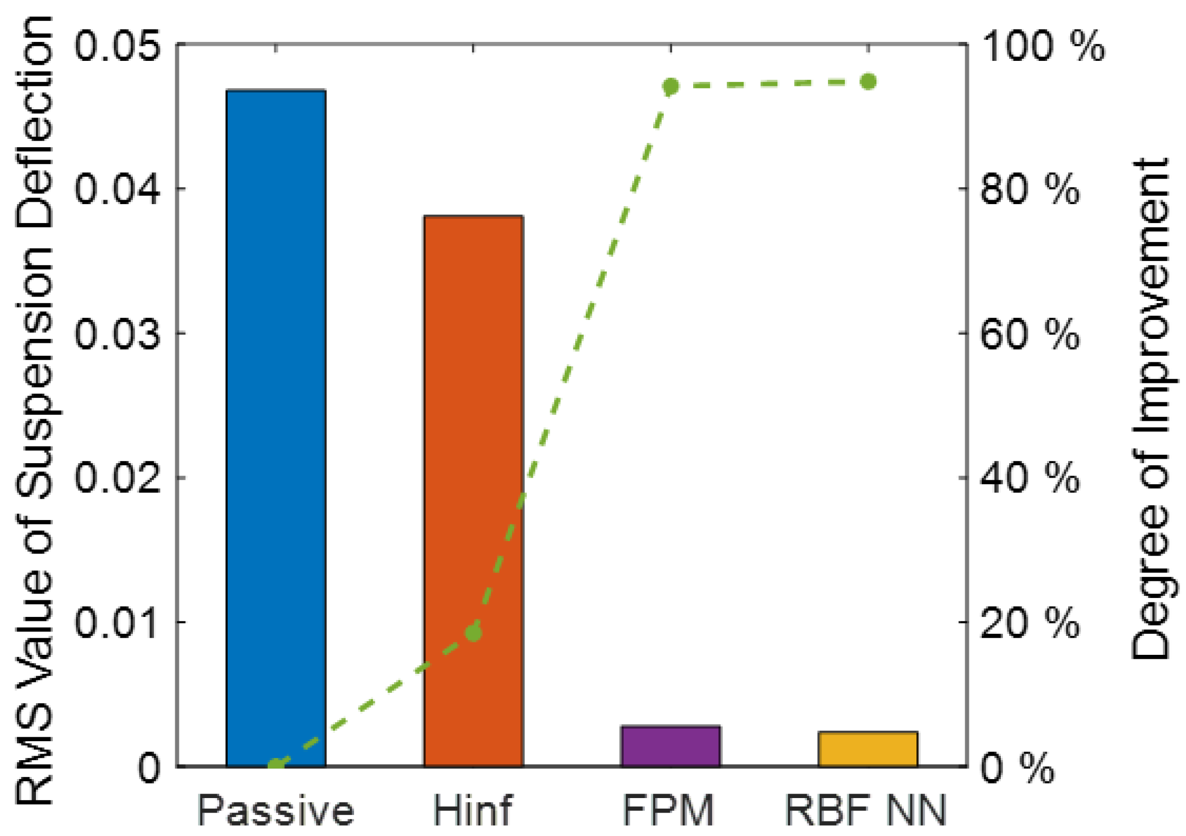
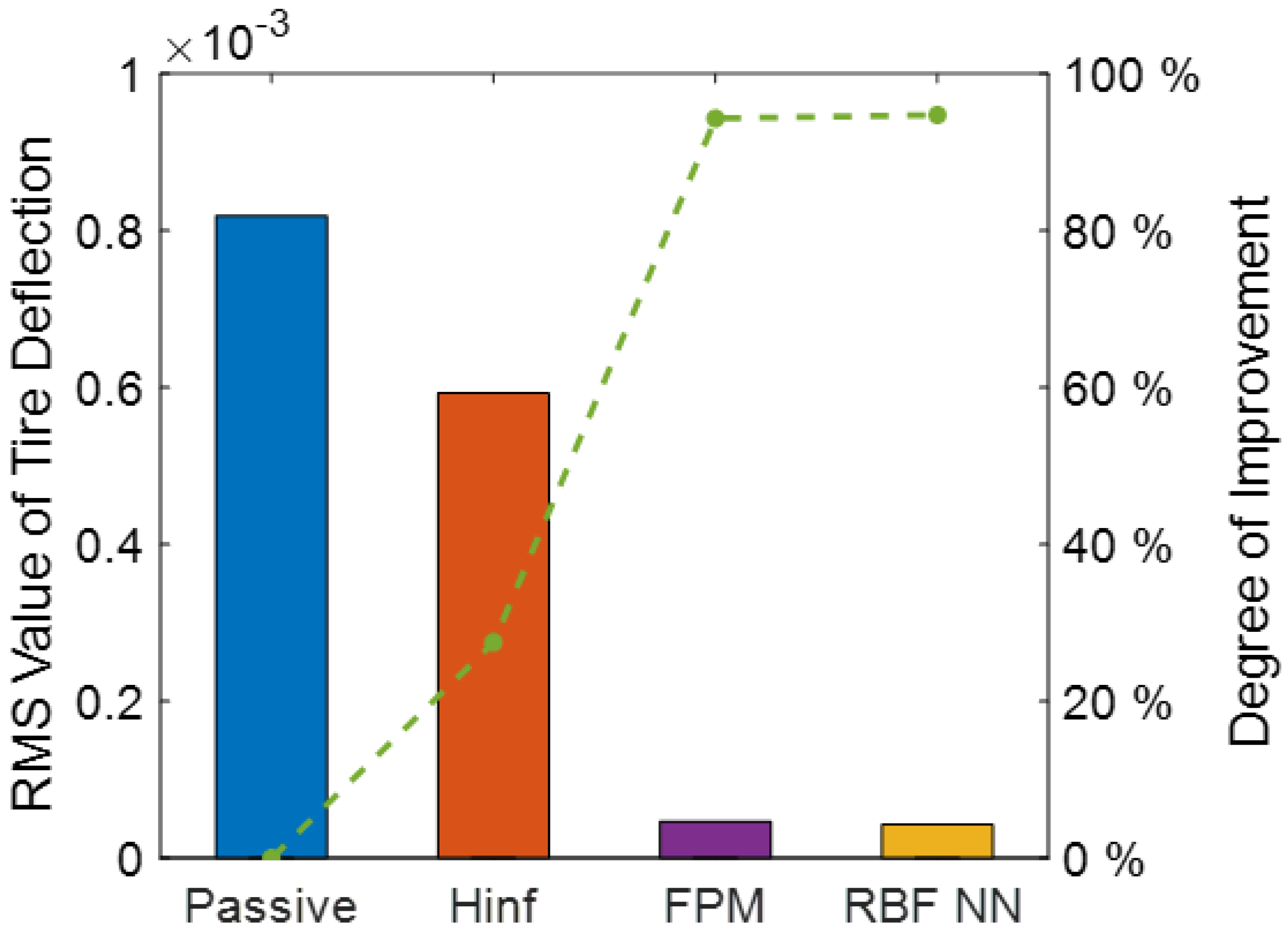
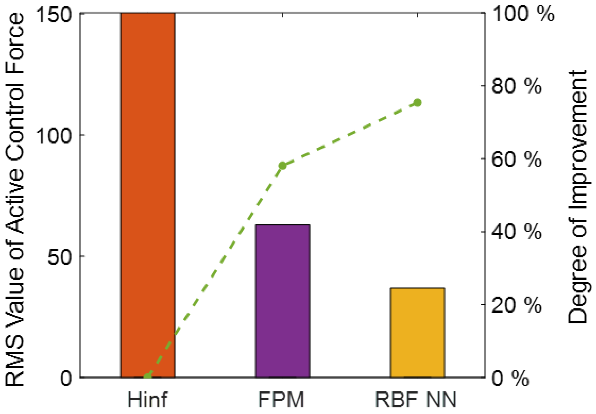
Sprung mass acceleration is usually used to evaluate the performance of passenger comfort. To evaluate the performance of driving stability, commonly used evaluation indicators include the deflection of the suspension and the deflection of the tire. The index RMS values used to evaluate the performance of suspension are presented in Figure 10, Figure 11, Figure 12 and Figure 13.

Figure 5 displays the sprung mass acceleration of the step response curves under $H_{\infty }$ and the proposed control method. Figure 5 shows that the amplitude of oscillation is smaller, the adjustment time is shorter, and the oscillations are fewer under the proposed controller compared with the $H_{\infty }$ method.

In Figure 6, car body acceleration is used to show the performance of these methods. According to Figure 6, the active suspension under the $H_{\infty }$ control method can obviously improve the performance in decreasing car body acceleration. However, the car body acceleration curve under the PID control using radial basis function neural networks is slower than the passive case, $H_{\infty }$ control, and FPM control method. This result demonstrates that the proposed controller performs better in terms of ride comfort than the other cases of the passive method, $H_{\infty }$ method, and FPM control method.

In Figure 7, the deflections of the vehicle suspension in the passive mode, adaptive PID control modes using the $H_{\infty }$ method radial basis function neural networks, and FPM control method, respectively, are presented. According to Figure 7, it can be seen that the deflection curve is slower under the $H_{\infty }$ control. However, the deflection curve regarding the suspension of the PID control using radial basis function neural networks is lower compared with the other cases. It illustrates that the proposed controller outperforms the other cases.

In Figure 8, the deflection values of the tire in the passive method, $H_{\infty }$ method, radial basis function neural networks, and FPM control method, respectively, are presented. According to Figure 8, it can be seen that the deflection curve of the tire is more smooth under the $H_{\infty }$ control. Nevertheless, the deflection curve regarding the tire of the PID control using radial basis function neural networks is lower compared with the other two cases of the passive and $H_{\infty }$ methods. Additionally, it illustrates that the proposed controller outperforms the others in terms of road holding.

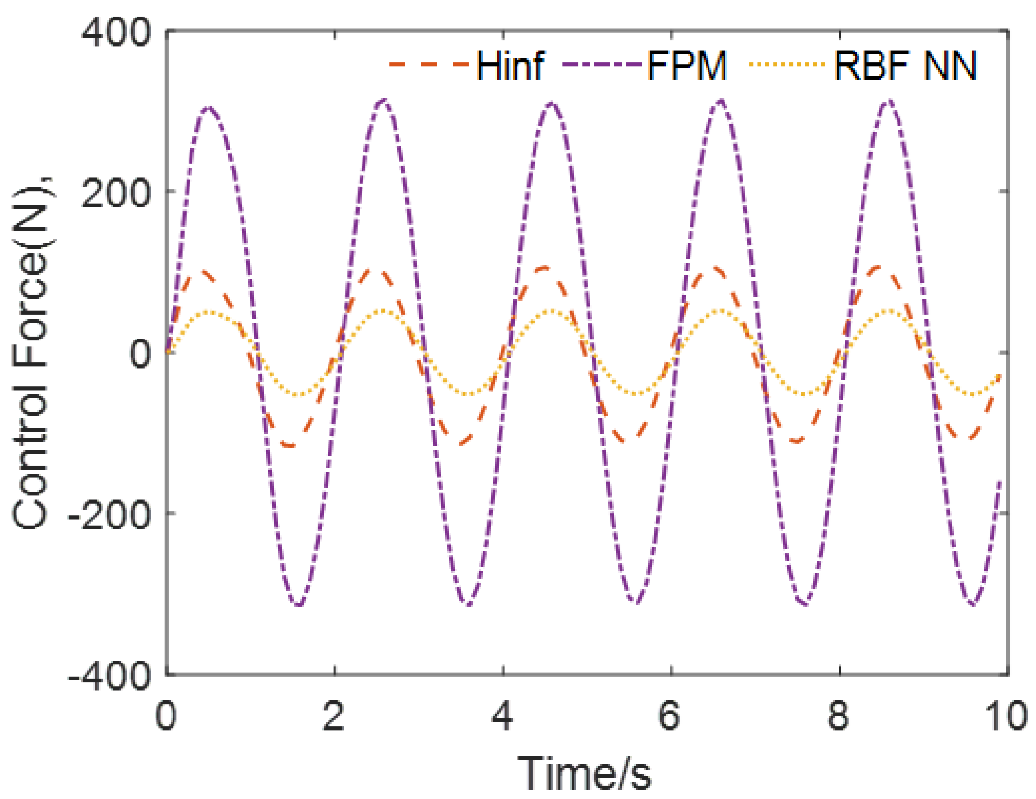
Figure 9 provides the control force curve produced by the actuator. And, as seen in Figure 9, the force curve produced by the PID control using radial basis function neural networks is smoother than the $H_{\infty }$ method. It can be said that the capability performance is more stable than other techniques.

The evaluation metric RMS values are shown in Figure 10, Figure 11, Figure 12 and Figure 13 and

Table 2. RMS value.

Evaluation Indicators	Passive	${\mathit{H}}_{\mathit{\infty }}$	FPM	Radial Basis Function Neural Networks
Sprung Mass Acceleration	0.6998	0.5032	0.047	0.0361
Suspension Deflection	$4.68\times {10}^{-2}$	$3.81\times {10}^{-2}$	$0.27\times {10}^{-2}$	$0.24\times {10}^{-2}$
Tire Deflection	$8.19\times {10}^{-4}$	$5.93\times {10}^{-4}$	$0.47\times {10}^{-4}$	$0.43\times {10}^{-4}$
Active Control Force	−	150.4	62.99	36.94

. Figure 10, Figure 11, Figure 12 and Figure 13 also present the raised premiums for suspension under the proposed control.

According to Figure 10, Figure 11, Figure 12 and Figure 13 and Table 2, the acceleration of the car body under a radial basis function neural networks-based PID control declines by 89%, 27.1%, and 23.2% compared with the cases of passive suspension, $H_{\infty }$ control, and the proposed compassion method with respect to the RMS value. In [25,26], it can be seen that the acceleration of the car body declines by 16.1% and 20.8% under the $H_{\infty }$ control method. The suspension deflection decreases by 94.8%, 52.9%, and 19.5% relative to the cases of passive suspension, $H_{\infty }$ control, and FPM control method with respect to the RMS value. In [25,26], it can be seen that the suspension deflection declines by 6% and 5% under the $H_{\infty }$ control method. The tire deflection drops by 94.7%, 52.7%, and 27.5%, in contrast to the cases of passive suspension, $H_{\infty }$ control, and the proposed compassion method with respect to the RMS value. The active force declines by 25% and 41.36% compared with the cases of $H_{\infty }$ control and the proposed compassion method with respect to the RMS value.

The $H_{\infty }$ control method has a better control performance. In [25,26], it can be seen that the acceleration of the car body declines by 16.1% and 20.8% under the $H_{\infty }$ control method. The suspension deflection decreases by 6% and 5%.

The results illustrate that the proposed controller exhibits significantly lower vertical acceleration, suspension dynamic deflection, and active force under sinusoidal excitation and exhibits significantly better vibration suppression than the other two suspension systems. Both smooth driving and stable handling are guaranteed. Additionally, it is demonstrated that the suspension can successfully improve stability in the presence of outer interference, demonstrating that its robustness has been significantly increased and showcasing the full potential of the car system with the proposed controller in enhancing the overall robustness of the vehicle.

Because of this, the suggested controller in this work may significantly minimize deflection and acceleration under the input case used in this research, further proving the effectiveness of the suggested strategy.

5. Conclusions

The PID controller has been utilized for a range of vehicle suspension controls and is widely recognized as the most frequently used controller in the industrial sector. It offers significant application value for enhancing the PID controller and addressing its issues.

To overcome the limitation that the parameters of PID control in classic active suspension control are defined by experience, and to dramatically accelerate learning while avoiding the local minimum problem, in this paper, the radial basis function neural networks technique was utilized to accelerate learning and prevent the local minimum problem. As a result, the adaptive PID control method based on radial basis function neural networks was used for active suspension control.

First, the quarter-car suspension model was taken into consideration. The radial basis function neural networks approach was applied to obtain the parameters of the PID; then, a simulation was conducted. The results were then collected in the MATLAB Simulink environment.

The results of the numerical simulation show that the proposed control strategy can significantly improve the performance of the vehicle when compared with passive suspension control, $H_{\infty }$ control, and the FPM method. According to the comparison, i.e., the control approach, the proposed technique can obviously have absolute road profile-tracking performance. It verifies the proposed control system’s reliability and efficacy. The proposed control algorithm’s capacity to reduce a large amount of vibration is an illustration of its effectiveness.

However, it should be noted that the suspension system is treated as an ideal model in this research, and friction and other outside interference elements are not taken into account. To better ensure driving safety, this study may be able to accommodate the needs of unique vehicles in complicated and varying road conditions. This is especially true for field roads. In future work, the real suspension system could be used for experimental simulations based on data obtained from real detection. In order to lessen vehicle suspension deflection and service wear, the results of road recognition should also be incorporated with other optimal algorithms.

References

- Yao, G.Z.; Yap, F.F.; Chen, G.; Li, W.; Yeo, S.H. MR damper and its application for semi-active control of vehicle suspension system. Mechatronics 2002, 12, 963–973. [Google Scholar] [CrossRef]
- Tamboli, J.; Joshi, A. Optimum Design of a Passive Suspension System of a Vehicle Subjected to Actual Random Road Excitations. J. Sound Vib. 1999, 219, 193–205. [Google Scholar] [CrossRef]
- Elmadany Mohamed, M.; Abdul Jabbar, Z.; Foda, M. Optimal preview control of active suspensions with integral constraint. J. Vib. Control. 2003, 9, 1377–1400. [Google Scholar] [CrossRef]
- Zapateiro, M. Vibration control of a class of semi-active suspension system using neural network and backstepping techniques. Mech. Syst. Signal Process. 2009, 23, 1946–1953. [Google Scholar] [CrossRef]
- Wang, D.; Li, C.; Liu, D.; Mu, C. Data-based robust optimal control of continuous-time affine nonlinear systems with matched uncertainties. Inf. Sci. 2016, 366, 121–133. [Google Scholar] [CrossRef]
- Al-Holou, N. Sliding mode neural network inference fuzzy logic control for active suspension systems. Fuzzy Syst. IEEE Trans. 2022, 10, 234–246. [Google Scholar] [CrossRef]
- Li, H.; Yu, J.; Hilton, C.; Liu, H. Adaptive Sliding-Mode Control for Nonlinear Active Suspension Vehicle Systems Using T–S Fuzzy Approach. Ind. Electron. IEEE Trans. 2013, 60, 3328–3338. [Google Scholar] [CrossRef]
- Basari, A.A.; Sam, Y.M.; Hamzah, N. Nonlinear Active Suspension System with Backstepping Control Strategy. In Proceedings of the IEEE Conference on Industrial Electronics & Applications IEEE, Harbin, China, 23–25 May 2007. [Google Scholar]
- Sun, W.; Gao, H.; Kaynak, O. Adaptive Backstepping Control for Active Suspension Systems with Hard Constraints. IEEE/ASME Trans. Mechatron. 2013, 18, 1072–1079. [Google Scholar] [CrossRef]
- Guo, L.X.; Zhang, L. Robust H∞ control of active vehicle suspension under non-stationary. J. Sound Vib. 2012, 331, 5824–5837. [Google Scholar] [CrossRef]
- Ang, K.H.; Chong, G.; Li, Y. PID control system analysis, design, and technology. Control. Syst. Technol. IEEE Trans. 2005, 13, 559–576. [Google Scholar]
- Kumar, M.S. Development of Active Suspension System for Automobiles using PID Controller. Adv. Mater. Res. 2008, 308–310, 2266–2270. [Google Scholar]
- Tejam, S.R.; Srinivasa, Y.G. Investigations on the Stochastically Optimized PID Controller for a Linear Quarter-Car Road Vehicle Model. Veh. Syst. Dyn. 2015, 26, 103–116. [Google Scholar]
- Han, S.-Y.; Dong, J.-F.; Zhou, J.; Chen, Y.-H. Adaptive Fuzzy PID Control Strategy for Vehicle Active Suspension Based on Road Evaluation. Electronics 2022, 11, 921. [Google Scholar] [CrossRef]
- Ji, X.; Li, S. Design of the fuzzy-PID controller for new vehicle active suspension with electro-hydrostatic actuator. In Proceedings of the IEEE Conference on Industrial Electronics & Applications IEEE, Xi’an, China, 25–27 May 2009. [Google Scholar]
- Venkateswarulu, E. The Active Suspension System with Hydraulic Actuator for Half Car Model Analysis and Self-Tuning with PID Controllers. Int. J. Res. Eng. Technol. 2014, 3, 415–421. [Google Scholar]
- Li, Y.; Wang, Z.; Ling, Z. Adaptive neural network PID sliding mode dynamic control of nonholonomic mobile robot. In Proceedings of the IEEE International Conference on Information & Automation IEEE, Harbin, China, 20–23 June 2010. [Google Scholar]
- Minh, C.H.; Kwan, K.A. Extended State Observer-Based Adaptive Neural Networks Backstepping Control for Pneumatic Active Suspension with Prescribed Performance Constraint. Appl. Sci. 2023, 13, 1705. [Google Scholar]
- Taghavifar, H.; Li, B. PSO-Fuzzy Gain Scheduling of PID Controllers for a Nonlinear Half-Vehicle Suspension System. SAE Int. J. Passeng. Cars Mech. Syst. 2018, 12, 5–20. [Google Scholar] [CrossRef] [PubMed]
- Nagarkar, M.P.; Bhalerao, Y.J.; Patil, G.J.V.; Patil, R.N.Z. Multi-Objective Optimization of Nonlinear Quarter Car Suspension System—PID and LQR Control. Procedia Manuf. 2018, 20, 420–427. [Google Scholar] [CrossRef]
- Yingwei, L.; Sundararajan, N.; Saratchandran, P. Performance evaluation of a sequential minimal radial basis function (RBF) neural network. IEEE Trans. Neural Netw. 1998, 9, 308–318. [Google Scholar] [CrossRef]
- Green, M.; Limebeer, D.J. Linear Robust Control; Courier Corporation: North Chelmsford, MA, USA, 1995. [Google Scholar]
- Hao, J.; Zhang, G. Data-Driven Tracking Control for a Class of Unknown Nonlinear Time-Varying Systems Using Improved PID Neural Network and Cohen-Coon Approach. In Proceedings of the 2021 IEEE 10th Data Driven Control and Learning Systems Conference (DDCLS), Suzhou, China, 14–16 May 2021. [Google Scholar]
- Radac, M.B.; Precup, R.E. Three-level hierarchical model-free learning approach to trajectory tracking control. Eng. Appl. Artif. Intell. 2016, 55, 103–118. [Google Scholar] [CrossRef]
- Zhang, W.; Yu, F. Study on Dynamics of Electromagnetic Active Suspension Based on Mix Robust Control. Mach. Des. Res. 2015, 31, 173–178. [Google Scholar]
- Wen, X. Design and Control Research of Electromagnetic Active Suspension Actuator. Ph.D. Thesis, ChongQing University, Chongqing, China, 2020. [Google Scholar]
Figure 1.
System model.
Figure 2.
PID control.
Figure 3.
The structure of radial basis function neural networks.
Figure 4.
Hybrid control flowchart.
Figure 5.
Sprung mass acceleration.
Figure 6.
Figure 7.
Vehicle suspension deflection.
Figure 8.
Tire deflection.
Figure 9.
Active control force.
Figure 10.
RMS value of sprung mass acceleration.
Figure 11.
RMS value of suspension deflection.
Figure 12.
RMS value of tire deflection.
Figure 13.
RMS value of active control force.