
UAV Path Planning and Obstacle Avoidance Based on Reinforcement Learning in 3D Environments


Department of Communications, Navigation and Control Engineering, National Taiwan Ocean University, Keelung 20224, Taiwan
*
Author to whom correspondence should be addressed.
Actuators 2023, 12(2), 57; https://doi.org/10.3390/act12020057
Submission received: 9 December 2022
/
Revised: 23 January 2023
/
Accepted: 23 January 2023
/
Published: 28 January 2023
(This article belongs to the Special Issue Intelligent Control and Robotic System in Path Planning)
Abstract
:This study proposes using unmanned aerial vehicles (UAVs) to carry out tasks involving path planning and obstacle avoidance, and to explore how to improve work efficiency and ensure the flight safety of drones. One of the applications under consideration is aquaculture cage detection; the net-cages used in sea-farming are usually numerous and are scattered widely over the sea. It is necessary to save energy consumption so that the drones can complete all cage detections and return to their base on land. In recent years, the application of reinforcement learning has become more and more extensive. In this study, the proposed method is mainly based on the Q-learning algorithm to enable improvements to path planning, and we compare it with a well-known reinforcement learning state–action–reward–state–action (SARSA) algorithm. For the obstacle avoidance control procedure, the same reinforcement learning method is used for training in the AirSim virtual environment; the parameters are changed, and the training results are compared.
1. Introduction
With the development of integrated circuit technology, rapid growth in computing power has led to a surge in the application of drones. Advances in microcontrollers have created a new world for many innovations. In recent years, work efficiency and human resources shortages have been extensively discussed. The use of drones will greatly reduce the death and injury of pilots flying planes, which is another great advantage of drones, so that research into drones has become more widespread. With the development of drones, some problems have been addressed or have evolved, such as aquaculture, infrastructure inspection, environmental monitoring, and agricultural spraying. Therefore, the development of path planning and obstacle avoidance systems needs to keep pace with the times, so that drones can effectively perform and complete automation tasks in various environments.
In recent years, unmanned aerial vehicles (UAVs) have gradually become an important issue in many studies; these are divided into two categories, comprising fixed-wing aircraft and multi-axis rotorcraft. The wing of a fixed-wing aircraft does not need to rotate and the aircraft uses the airflow passing around the wing to provide lift. Fixed-wing aircraft can only fly forward and cannot fly in any other direction. In addition, fixed-wing aircraft are unable to make an immediate sharp turn or to fly backward. Furthermore, the runway for fixed-wing aircraft must be long enough for them to be able to take off as well as to land. Conversely, the rotorcraft, also known as the multirotor, has the capacity for vertical take-off and landing (VTOL); it can thus enjoy unlimited movement and freedom in the air. The multirotor can hover above the target location and can drop items of set weight within the load range for delivery to the designated location. The application of this study is to use unmanned multi-rotor aircraft to replace traditional human operations. The multirotor can drop sensors to collect environmental information from the cage net in the ocean for the purposes of aquaculture. In order to carry out this mission, making the UAV fly safely to its destination is the most important issue. The main purpose of this study is to plan appropriate paths and design an obstacle avoidance system to ensure that the UAV has a safe flight to its destination.
In past decades, the most frequently used path-planning algorithms include Dijkstra’s algorithm, A Star (A*), and D*. Dijkstra’s algorithm and A* plan the projected path from the starting position to the goal position. A* also considers the distance from the starting position to the goal [1]. D* plans the path by setting off from the goal to the starting position. It has the ability to adjust the projected path in the face of obstacles [2]. Although these algorithms can successfully plan paths, the drawback is that they are computationally expensive when the search space is large. Rapidly exploring random tree methods represents a less expensive approach because it can quickly explore a search space with an iterative function [3]. Still, these algorithms are time-consuming and may not be appropriate for UAVs. The main objective of path planning is to have less computational time needed for optimal path planning. The path generated by the path-planning algorithms should be optimal so that it consumes minimal energy, takes less time, and reduces the likelihood of collisions between UAVs and obstacles. Classical algorithms cannot truly reflect the actual needs of UAV path planning. In this paper, a UAV path-planning algorithm, based on reinforcement learning, was applied according to the simulated scenarios. The UAV can follow this planned path and perform visual real-time collision avoidance by the use of depth images and deep-learning neural networks.
The UAV can either be operated by the operator visually, or the operator can wear special glasses to fly in first-person view (FPV) mode. In addition, one can write code to use a microcontroller to operate the UAV. The traditional control-system technology uses a PID controller to give the flight attitude of UAVs good performance [4,5]. In addition, the adjustment of PID parameters, based on reinforcement learning, has been proposed by the authors of [6,7]. In recent years, the use of drone applications in many fields has become more and more common. T. Lampersberger et al. proposed the application of a radar system and antenna in UAVs [8]. P. Udvardy et al. used drones to model a church in 3D and evaluated the results [9]. In [10], Z. Ma et al. discussed communication research using UAVs in an air-to-air environment. K. Feng et al. used UAVs for package delivery research [11]. Among these applications, UAV path planning and obstacle avoidance issues are worthy of study and discussion. In addition, research into the applications of reinforcement learning is also very popular. For example, Alphago is a well-known reinforcement learning application [12]. In other studies [13,14,15,16], research based on the Q-learning algorithm was applied to path planning. A. Anwar et al. used reinforcement learning methods to study obstacle avoidance control [17]. The final research results are amazing, and the content produced is excellent. In [18,19,20,21], many deep reinforcement learning methods for obstacle avoidance were proposed and the results were analyzed. With the help of a number of reinforcement learning experiences, this study proposes a comparison of path planning based on the SARSA algorithm and the Q-learning algorithm in reinforcement learning, along with the use of a deep Q-learning algorithm for obstacle avoidance simulation experiments.
A brief introduction to path planning and obstacle avoidance, based on reinforcement learning, was presented in [22]. In this study, a detailed description and extension methods are presented. The proposed methods are divided into two parts. The first part concerns path planning. In path planning, we compare the Q-learning algorithm with the SARSA algorithm. The principles of these two algorithms are similar, but they still have their own characteristics. Therefore, we propose two reinforcement-learning methods for path-planning experiments. In the second part, obstacle avoidance control is utilized; because the input depth image data is more complicated, deep Q-learning is used for experiments, then the training results are observed in a simulated environment. Considering the future testing of reinforcement learning methods involving physical drones, we use ultrasonic sensor modules to assist in side-obstacle avoidance, so that the drone can maintain a safe distance from obstacles. This study applies reinforcement learning methods to train the UAV in a simulated environment, followed by testing and then analysis of the results.
2. System Description
In this study, a hexacopter was used to perform an assigned task, for instance, to collect sensor data for the purposes of aquaculture. This section details the main architecture, sensors, and computer hardware configuration used in deep-learning training. The computational hardware system includes an onboard computer and off-line training computer. The basic UAV system consists of a flight control board, power supply, sensors, motors, 3DR telemetry radio, and a remote controller. At the ground control station, the operator can send control signals to the flight control board via the remote controller and obtain flight status information from the Mission Planner software, which communicates with the 3DR telemetry radio device. For UAV systems, sensors such as accelerometers, barometers, and gyroscopes are used to monitor changes in the environment to maintain flight stability; then, the environmental information is sent back to the flight control board to adjust the flight attitude of the hexacopter. Figure 1 shows the UAV’s system structure.
The flight control board of the hexacopter is the Pixhawk 4, which is part of an independent open-source project. It has a more advanced 32-bit ARM Cortex® M7 processor, 16 PWM/servo outputs, and others used to establish the flight status. The necessary sensors include a three-axis gyroscope, barometer, magnetometer, and accelerometer. The attitude of the hexacopter can be improved by the two sets of accelerometers, while other sensors can help the hexacopter to locate its position. In order to prevent positioning errors, the Pixhawk 4 can also have the compass and GPS module installed externally, away from the motor, electronic speed controller, and power supply lines.
The ground control station (GCS) software and the flight control board work together, and the appropriate firmware version can be selected and installed. The operator can easily obtain the flight information via the Mission Planner software, which helps the operator to understand the current rotorcraft status and record the flight data during the mission at the same time. This allows us to acquire information if the hexacopter had crashed or encountered other emergency situations. The NEO-M8N module is highly compatible; therefore, it is widely used in UAV positioning systems. GNSS can concurrently receive GPS, Galileo, GLONASS, and Beidou satellite signals, accessing them all at the same time. The safety switch of the drone hardware is also on the same module. In a favorable area without obscuration and interference, the NEO-M8N module, when combined with real-time kinematic (RTK) positioning technology, can receive data from up to 30 satellites; the horizontal dilution accuracy (HDOP) is often between 0.5 and 0.6, which means that the GPS is in good condition; that is, the positioning error (static) is less than 10 cm.
The accuracy of waypoints in path planning is very important. In this study, the RTK positioning technology is used. RTK base stations are set up in the experimental field to wait for their convergence and are then connected to the chip on the hexacopter, so that the error can be reduced to 10 cm. Figure 2 shows the ground station of the RTK. The working procedure of the proposed approach is shown in Figure 3.
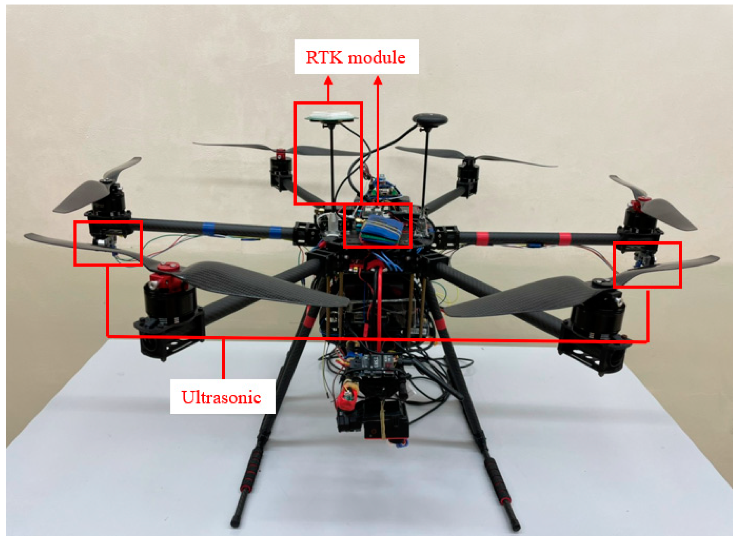
In this study, we used a self-assembling hexacopter, which is mainly made from lightweight and strong carbon fiber. Compared with the quadcopter, the hexacopter utilizes a sensor that is more resistant to strong wind interference and offers greater force-bearing. The main body of the hexacopter is shown in Figure 4. The on-board computer is used for the path-planning experiment and obstacle-avoidance experiment. Ultrasonic sensors are set on the side of the hexacopter. The hexacopter is also used in aquaculture projects, considering that we can implement reinforcement learning algorithms in the future for hexacopter obstacle avoidance and other tasks that require a lot of computing to detect objects. For integration, we used the NVIDIA Jetson Xavier NX development kits and modules. The use of deep Q-learning in the virtual environment of Microsoft AirSim requires a great deal of computer resources; therefore, a graphics card with better graphics computing capabilities and sufficient memory, etc. is required. The sensor used for obstacle detection on the side of the UAV’s body is the ultrasonic ranging module, HC-SR04. The HC-SR04 has a ranging accuracy of 3 mm and can measure distances from 2 cm to 400 cm.
3. Path Planning
One of the most complex problems that are widely explored in robotics concerns path planning. There are many algorithms that have been applied to path planning, such as the improved ACO [23], used to navigate in a maze-like environment, the ACO combined with chaos theory [24], used to find a path away from threatened areas, and the improved PSO [25], used to navigate a ship in the surrounding environment of an island. When the hexacopter performs tasks, there are often huge static obstacles in the execution area, such as mountains, buildings, no-fly zones (NFZ), etc. Pathfinding in a known environment is known as global path planning. The main purpose is to spend less time and reach the destination without passing through restricted areas. Compared with the traditional A* algorithm, the reinforcement learning algorithm can solve more complex problems. However, when the model corrects the error, the chance of the same error is very small. This technique is the first choice for long-term results. This method can collect information about the environment and interact with the specific environment of the problem, which makes this method of problem-solving flexible. The learning model of reinforcement learning is very similar to that of human learning. Therefore, this method will be closer to perfect expectations. In this section, all obstacle settings are treated as a priori information, which represents a known environment. Before the hexacopter takes off, we calculate the path and plan the best path. Using the known information, two search algorithms based on reinforcement learning are applied to generate optimal routes in this study. As a result, the hexacopter can fly through the given waypoints. The introduction of these two algorithms is given as follows.
3.1. Markov Decision Process (MDP)
In reinforcement learning, the three basic elements are state, action, and reward. These three elements are the messages that the agent and environment communicate with each other, but they still lack communication channels, as shown in Figure 5. This pipeline is created through the mathematical model of the Markov decision process (MDP) [26].
The agent interacts with the environment, as shown in Figure 5. The environment gives the state and reward at time t to the agent, and the agent then determines the behavior to be performed using this information. Then, the environment determines the state and reward for the next time through the behavior of the agent. All the processes of MDP are random and the next state transition is only related to the current state. At time t, action is made according to , and the state at the next time, + 1 is uncertain. We call this environment transition probability the MDP dynamic. The equation is as follows:
After taking action in the state , the probability id that the next state is and the reward is . The next-state transition of MDP is only related to the current state; we call this the Markov Property, which can be expressed using the following equation:
The current state contains information about all the states experienced in the past. However, the probability that we are looking for can reject all the past states and focus only on the present state. This greatly reduces the amount of calculation necessary, and we can then use a simple iterative method to find the result. However, since not all reinforcement-learning problems satisfy the Markov property, we can assume that the Markov property is satisfied to achieve approximate results.
3.2. Bellman Equation
The Bellman equation [27] is also called the dynamic programming equation. Many common reinforcement learning algorithms are based on the Bellman equation, and the goal of reinforcement learning can be expressed as a value function. Calculating the solution of this value function can indirectly identify the best solution for reinforcement learning. However, the solution of the value function must be simplified by the Bellman equation. The Bellman equation is as follows:
where represents the immediate reward values and is the discount factor (). However, it is uncertain, when moving from state to state , if there will be an expectation symbol in the outermost layer. By observing the equation, we can see that v(s) is composed of two parts. One is the immediate reward expectation of this state. According to the definition of the immediate reward, this will not be related to the next state. The other is the value expectation of the state in the next moment, which can be obtained according to the probability distribution of the state at the next moment. If is expressed as any possible state at the next moment in state , then the Bellman equation can be written as:
The value function of each state is calculated iteratively through the Bellman equation. Below, we give an example showing the calculation of the value function of a state to help with understanding the process, as shown in Figure 6.
After substituting the value into the calculation of Equation (4), the value of the current state can be obtained, as shown in Equation (5):
However, when the current state is 4.3, the subsequent state value function is 0.8 and 10. In fact, these values can be arbitrarily initialized and updated through learning, thereby functioning in the same way as the weight parameters in neural networks. They are initialized arbitrarily at the beginning of the process and are then updated backward through loss.
3.3. Policy
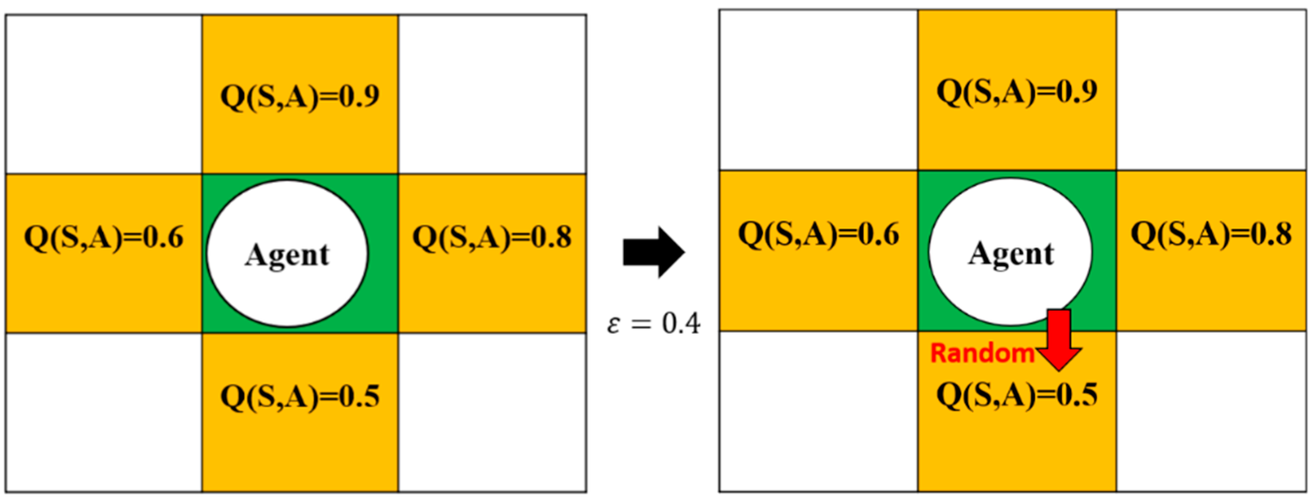
In both the Q-learning algorithm and the SARSA algorithm, a particular policy is required for action selection. In this study, two policies were applied and are introduced here. The first is the most intuitive, the greedy policy [28]. Assuming the situation encountered below is shown in Figure 7, there are 4 directions to choose from in this state, and the highest 0.9 Q-value is selected according to the Q-table; this is the greedy policy mentioned above, to which we add random probability. In this way, during the training process, there is a chance that the agent of ε will choose a random direction, so that the model has the opportunity to learn new experiences. This is the ε-greedy policy [29].
In Figure 8, there is a probability that the agent in this state will randomly choose the direction so that the agent has the opportunity to learn new experiences and will not always choose the same action.
3.4. Q-Learning Algorithm
Q-learning is a time difference (TD) method and is also a classic method in reinforcement learning [30]. The Q-learning algorithm uses the newly obtained reward and the original Q-value to update the current Q-value, which process is also called value iteration. Then, it creates a Q-table and updates the Q-table with the rewards of each action, as shown in Algorithm 1. The Q-learning algorithm procedure is shown in Figure 9. The inputs of this algorithm are state S (the current position coordinates on the map), action A (the direction of movement), and reward R (the reward from the current position to the next position). The outputs are the values of the Q-table.
| Algorithm 1 Q-learning (off-policy TD control) for estimating |
| Initialize arbitrarily, and Repeat (for each episode): Initialize S Repeat (for each step of episode): Choose A from S using policy derived from Q (e.g.,-greedy) Take action A, observe R, ; until S is terminal |
The Q-learning algorithm is off-policy. This different policy means that the action policy and the evaluation policy are not the same. The action policy in Q-learning is the ε-greedy policy, whereas the policy to update the Q-table is the greedy policy. The equation for calculating the Q-value is as follows, and is based on the Bellman equation:
where represents the reward values that are obtained from state to state , is the learning rate (), and is the discount factor (). When the -value is larger, the agent pays more attention to the long-term rewards to be obtained in the future. Finally, the calculated Q-value is stored in the Q-table. The flowchart is shown in Figure 10.
3.5. Reward
In the process of human learning and growth, parents will teach their children what things should be done, or what things are dangerous and should not be done. The right actions will be rewarded, and the dangerous actions will be punished. In Q-learning, it is also necessary to set reward and punishment rules. In this way, when iterating and updating the Q-value, the result will be closer to expectations. When we initialize the reward, the reward rules are as shown in Equation (7). Finally, in order to reach the goal with the least number of steps, each step will be taken as −1. The schematic diagram of the reward and punishment rules is shown in Figure 11. The rules are flexible and need to be adjusted according to the problem. In other words, the rules of reward and punishment depend on the problem. Q-learning will thus maximize the overall reward as much as possible. Therefore, there is more than one route in Figure 12 that will yield the highest score.
The ultimate goal of Q-Learning is to obtain feedback, meaning that the sum of all rewards on the trajectory during the training process needs to be saved. Therefore, the Q-table of the two-dimensional table is designed to store the , which can store the expected maximum reward value for each action in each state in the future. In this way, we can know the best action for each state. The table is known as the Q-table and is shown in Figure 13.
There are four actions in the Q-table in the grid map (up, down, left, and right actions). The row represents the state, while the value of each cell will be the maximum reward value expected in the future for a specific state and action.
3.6. State–Action–Reward–State–Action (SARSA) Algorithm
SARSA is also a time difference (TD) method and is a classic method in reinforcement learning [31]. The SARSA algorithm is similar to the Q-learning algorithm; the main difference is the way in which it updates the Q-value, as shown in Algorithm 2. The SARSA algorithm procedure is shown in Figure 14. The inputs of this algorithm are state S (the current position coordinates on the map), action A (the moving direction), and reward R (the reward for moving from the current position to the next position). The outputs are the values of the Q-table.
| Algorithm 2 Sarsa (on-policy TD control) for estimating |
| Initialize arbitrarily, and Repeat (for each episode): Initialize S Choose A from S using policy derived from Q (e.g.,-greedy) Repeat (for each step of episode): Take action A, observe R, Choose from using policy derived from Q (e.g.,-greedy) until S is terminal |
This algorithm mainly incorporates the five elements of reinforcement learning: state (S), action (A), reward (R), discount factor, , and exploration rate, , and uses the optimal action value function to find the best path. It can be seen that in the updated formula of , the on-policy update method is adopted, and both the action policy and the update policy are an ε-greedy policy. This means that the SARSA algorithm will directly adopt the policy that is currently considered the best in the current state. The equation for calculating the Q-value is as follows:
where represents the reward values that are obtained from state to state , is the learning rate (), is the discount factor (). Finally, the Q-value is updated and stored in the Q-table via an iterative calculation.
3.7. SARSA Algorithm, Compared with the Q-Learning Algorithm
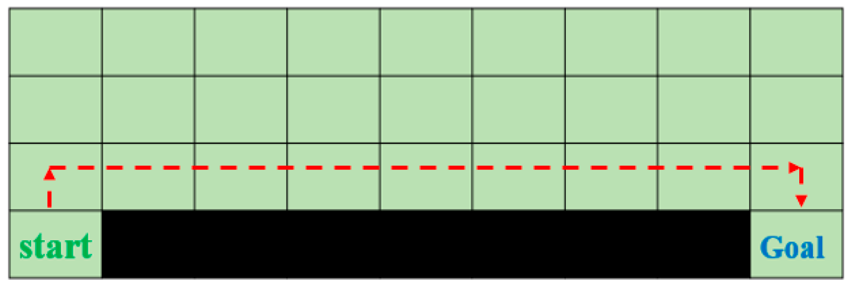
Comparing the two algorithms in the grid world shows that there will be different paths due to the different Q-value update methods. An example is shown in Figure 15.
In this environment, one point is lost for every square moved. When stepping into the black area (obstacle), the algorithm will lose one hundred points and return to the starting point. Finally, it will learn the path with the highest score to reach the goal. The method uses both the SARSA algorithm and Q-learning algorithm for learning. The results are shown in Figure 16 and Figure 17; the dashed line is the optimal route of each algorithm.
The action policy of the Q-learning algorithm is based on the ε-greedy policy; only the globally optimal action is considered in the Q-value update method. The SARSA algorithm can only find a suboptimal path, which is intuitively safer. Because the SARSA algorithm has the same action policy and evaluation policy, it considers the possibilities of all actions (ε-greedy). When it is close to the black area, there is a certain probability that it will choose to take a step toward the black area, so it is less likely to choose the path around the black area. Although the Q-learning algorithm has the ability to learn the globally optimal path, its convergence is slow, while the SARSA algorithm has a lower learning effect than the Q-learning algorithm, but its convergence is faster and simpler. Therefore, we need to consider the different issues.
4. Obstacle Avoidance
In recent years, drones have become popular in both the consumer and professional fields. Therefore, great research attention has been paid to the obstacle-avoidance function of UAVs. In order to ensure flight safety, although drones have GPS signals, there are still some small static or dynamic obstacles, such as trees, walls, and birds. None of these obstacles can be ascertained from the GPS data. In order to solve this problem, the obstacle avoidance system first needs accurate positioning information of the UAV, relative to the obstacle. Several methods have been proposed, such as the use of deep reinforcement learning, based on obstacle avoidance training and testing in a virtual environment [18,32], or the use of depth cameras with computer vision detection to avoid obstacles [33,34]. After obtaining information about the environmental obstacles, the UAV will adopt the corresponding avoidance direction and keep the flight stable. The main purpose of the current research is to collect water-quality information regarding the cage net in the ocean. Therefore, several long obstacles of sufficient height have been placed to simulate the situation when encountering sails at sea. The ground also has up- and down-slopes to simulate the environment of sea waves. The following describes the system architecture and the details of training in a virtual environment.
In the previous section, we mentioned the Q-learning algorithm. First, we suppose that when a complex problem is encountered, the Q-table needs to store very large quantities of states and actions. This will slow down the training speed and reduce the effect. Obstacle avoidance is a complex problem of this type. Therefore, a neural network is used for the calculation of the Q-value, known as the deep Q-learning network (DQN). The relationship of the DQN with the environment is shown in Figure 18. The inputs of the deep neural network are the depth images from the UAV’s side. The outputs of the deep neural network are the Q-values.
4.1. Deep Q-Learning Algorithm
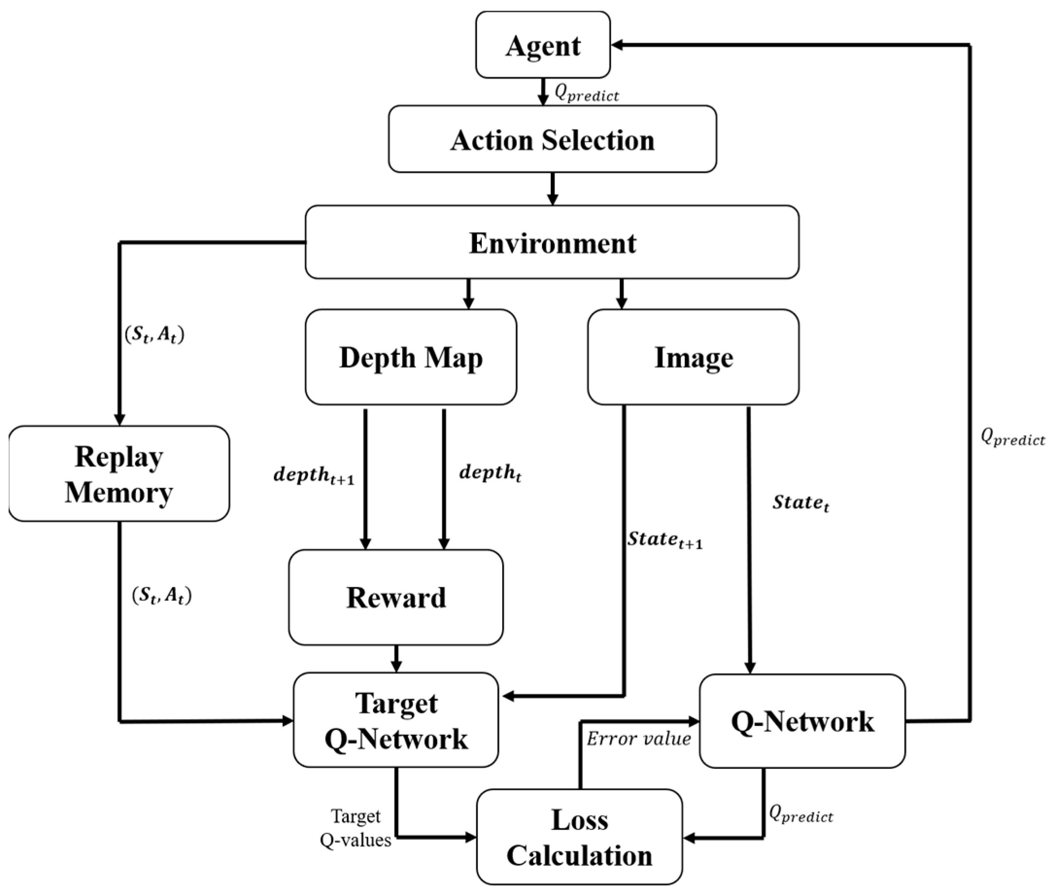
The deep Q-learning algorithm was originally designed for a brick-and-mortar game [35]; it is a method for passing Q-learning through the approximate value function of a neural network. It has achieved results that surpass human-level players in the Atari 2600 game; the algorithm is also suitable for the problem of avoiding obstacles. DQN has two models with the same structure; one is a Q-network and the other is a target Q-network. The parameters of the target Q-network will remain for a set period of time, the purpose of which is to avoid algorithm divergence. The DQN algorithm will update the Q-network parameter value to the target Q-network after a certain period of time. The DQN algorithm diagram is shown in Figure 19.
The core of DQL is the error between two neural networks. According to the target network, we should select the action with the largest Q-value and the corresponding We then multiply the discount factor, , by this maximum value and add r, to establish the target value of the neural network. The square error between the target value of the target Q-network and of the Q-network is the error of the deep neural network. Finally, we use the error calculated by the loss function to train the neural network. The inputs of this algorithm are state s (image pixel information), action a (moving direction), and reward r (the reward for moving from the current position to the next position). The outputs are the values of the Q-table. The DQL algorithm is shown as Algorithm 3 [35].
| Algorithm 3 Deep Q-learning with Experience Replay |
| Initialize replay memory D to capacity N Initialize action-value function Q with random weights For episode = 1, M do Initialize sequence and preprocessed sequenced for t = 1, T do With probability select a random action select a random action otherwise select Execute action in emulator and observe reward and image Set ,, and preprocess Store transition (,,,) in D Sample random minibatch of transitions (,,,) from D Set Perform a gradient descent step on according to Equation (3) end for end for |
The reason for experience replay is that the deep neural network, as a supervised learning model, requires the data to meet independent and identical distributions. The samples obtained by the Q-learning algorithm are related to the data both before and after. In order to break the correlation between these datasets, the experience replay method breaks this correlation via storage and sampling. The following equations are the equation of the gradient descent method and the equation for the loss function:
The stochastic gradient descent method can be used to optimize the weight, minimize the loss function, and gradually approach the optimal Q function to satisfy Bellman’s equation. If the loss function is 0, it can be considered that the approximation function has reached the optimal solution.
4.2. Microsoft AirSim Environment
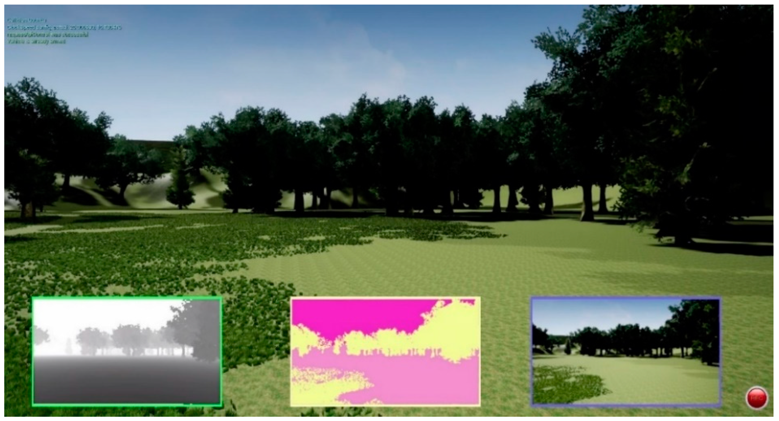
AirSim [36] is an open-source platform for drones, cars, and other simulators that were built based on Unreal Engine 4. It can also offer a cross-platform for simulation control through the PX4 flight controller. AirSim can interact with vehicles or drones in the simulation program via programming languages, such as Python, and can use these APIs to retrieve images and obtain the status to control the vehicle. The use of reinforcement learning methods for UAV obstacle avoidance training requires multiple collisions. Training in the real world will inevitably take a great deal of time and cost, and it will also cause doubts about flight safety. Therefore, most of the reinforcement learning training will be carried out in a virtual environment. In this study, we presented the obstacle avoidance results within the AirSim virtual environment. The environment from the AirSim is shown in Figure 20.
4.3. Obstacle Avoidance System in the AirSim Environment
A particular variable, D, known as replay memory, is used in the DQL algorithm to store the current state, current action, current action reward, and next state. When training the neural network, we randomly select batch-size samples from variable D to train the neural network. In this study, there are an RGB camera and a depth camera in front of the virtual drone. In the case of drones, the RGB image is the current state feature, and the depth image is used to obtain the distance information regarding the surrounding obstacles and to obtain the rewards for the current action selection. The DQL obstacle avoidance flow chart is shown in Figure 21.
We use the backpropagation method, by means of the error between the target value and the current value, to train the neural network. After that, we output the best predicted Q-value for action selection. Figure 22 shows the neural network architecture. The image adopts 227 227 3 as the input; it passes through the convolutional network layer for feature extraction, then passes through the fully connected layer for classification, and finally outputs 25 Q-values for each action selection.
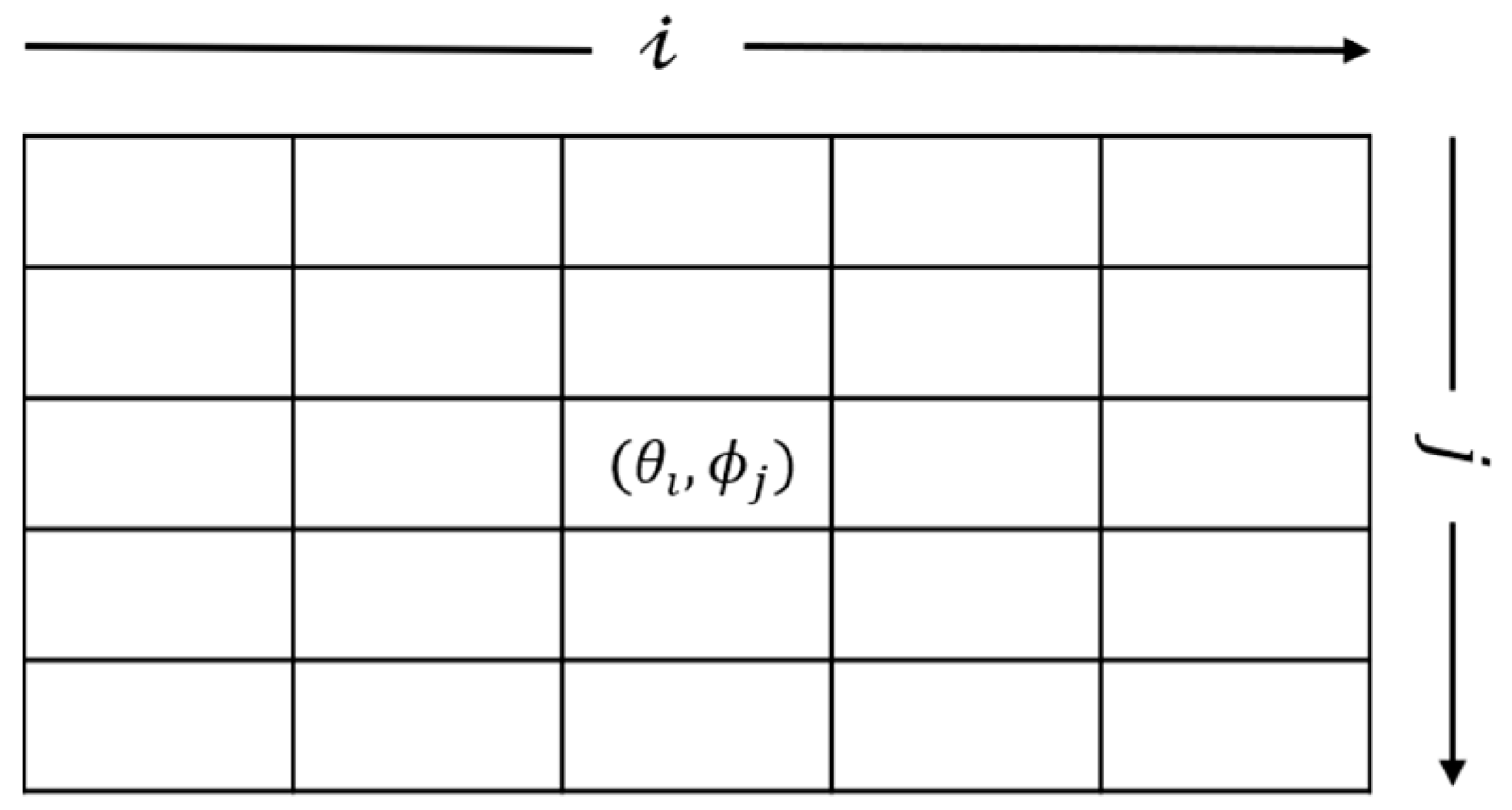
The action space is a 5 5 size, as shown in Figure 23. There are 25 action options; the flight action of the drone is calculated via angle equations, then we output the pitch and yaw control commands to the UAV. and represent the moving angles for the horizontal and vertical directions. These angle equations are calculated as follows:
where and are the locations, as shown in Figure 23. The size of the action space is N N. and are information on the horizontal and vertical attitudes, respectively, taken from the drone.
4.4. Ultrasonic Sensor
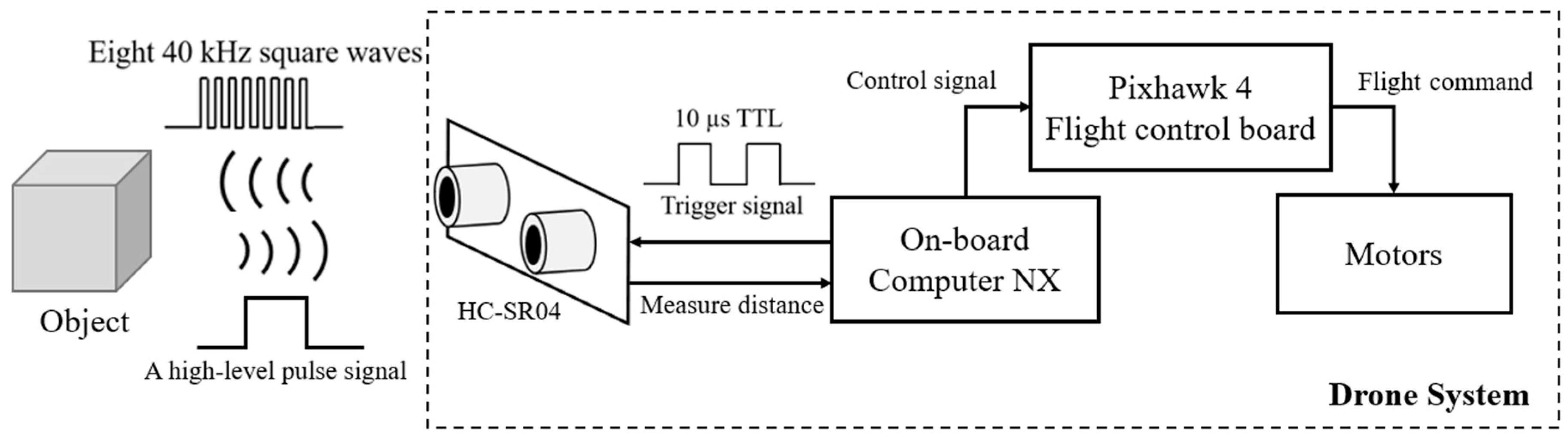
The principle behind employing the HC-SR04 to measure distance is to use an I/O trigger to send a high-level pulse signal of more than 10 μs, so that 8 periodic 40 kHz square waves are automatically generated in the module; we then wait for the receiver to detect the signal after the bumped object rebounds it, as shown in Figure 24.
The equation of the sound velocity in air, with the temperature in degrees Celsius, can be written as follows:
Therefore, the distance to the object can be estimated according to the time when the sound wave travels back. We assume that the temperature is 25 degrees Celsius and that the air condition of the environment is dry; after calculating the sound wave velocity equation, which is mentioned above, we can achieve 346.5 m/s or 0.03465 cm/µs, which means that the time the sound wave takes per centimeter is about 28.86 microseconds. Then, according to the width of the high-level pulse signal, which is proportional to the detection distance, the distance, from the object is given as follows:
Here, in order to make the distance measured by the ultrasonic sensor module more stable, the received measurement value is filtered. This filtering method was first proposed by the authors of [37].
The steps are as follows.
- Step 1.
- Set the maximum tolerance as 0.3 cm.
- Step 2.
- Send impulse signal and get five data each time from the ultrasonic sensor, then add in the temporary data list.
- Step 3.
- Sort the received data and calculate the median value of the data list.
- Step 4.
- If there is a previous value, go to step 5, or go to step 6.
- Step 5.
- Calculate the difference in the current value and the previous value; if the difference is bigger than the maximum tolerance, then the output is equal to the previous result, plus or minus the maximum tolerance.
- Step 6.
- Record the current value as the previous value and output the result and go to step 2.
Comparing the original measurement distance with the filtered measurement distance, it is obviously improved, and the value can be stabilized for different distances. The different distances are compared, and the error and the time consumption are calculated. The data are shown in Table 1. However, the ultrasonic sensor module has a chance of becoming stuck; the measure values were stopped at the same value. The steps for the solution are presented as follows:
- Step 1.
- Set to enter the protection mode when the output value is continuous and the same.
- Step 2.
- Save 30 values to the temporary data list.
- Step 3.
- Compare the first 29 items of data with the last 29 items of data in the temporary data list.
- Step 4.
- If the values are the same, close and restart the measurement.
Finally, after stabilizing the measured value of the ultrasonic sensor, the UAV must perform an avoiding distance maneuver, in the opposite direction and then output different drone speeds, according to the measured distance, . The ultrasonic dodge rules are set as follows:
5. Experimental Results
This section is divided into three parts. The first is used to compare the path-planning part in the grid world and use a better algorithm to fly in the real world. The second is an experimental flight with ultrasonic-assisted obstacle avoidance in the real world. The last part is intended to demonstrate the dodge test in a simulated forest environment after the reinforcement learning training is completed.
5.1. Path Planning
Both SARSA and Q-learning are algorithms based on MDP. The two are very similar, and so they are often compared. In Experiment 1, we observed the path difference of the two algorithms in the same grid world, as shown in Figure 25.
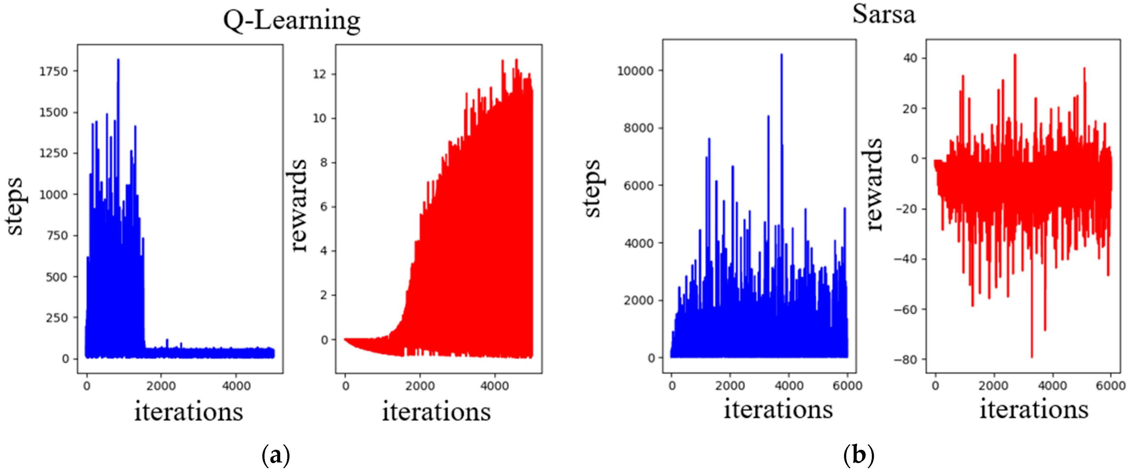
As can be seen from the above figures, the path of the Q-learning algorithm is significantly better than that of the SARSA algorithm. In Figure 26a, it can be seen that the reward part of the Q-learning algorithm is obviously higher and is higher with respect to iteration, and the number of steps in the exploration target gradually converges. Conversely, the SARSA algorithm shows no significant reduction in the number of steps to explore the target and may fall into a local optimum, as shown in Figure 26b. Although the reward part has a high score, it is not stable. In Figure 24, the reward points after the iteration are gradually accumulated, and the reward point of the last iteration is the sum of the maximum value and the minimum value. Figure 27 shows the Q-table after training in Environment 1. In the process of updating the Q-value, the Q-learning algorithm will select the action with the largest Q-value among all the actions in the next state. The SARSA algorithm is more intuitive in terms of choosing the best action that is currently considered; the Q-learning algorithm will try to maximize the overall benefit. Therefore, it is more suitable for exploring this type of path-planning problem, which only has starting-point and end-point information, with unknown environmental obstacle information. The path length and exploration time are shown in Table 2.
In the second experiment, the obstacles in the grid world have been changed. The central part is blocked by new obstacles and the path becomes narrow just before the target point. The path of the SARSA algorithm is shown in Figure 28a, and the path of the Q-learning algorithm is shown in Figure 28b. The path of the Q-learning algorithm is still better than that of the SARSA algorithm.
More obstacles are in place in Environment 2; therefore, the task of finding the best path becomes more difficult. In terms of rewards, the Q-learning algorithm still maintains the maximum benefit for exploration, and the difference from the SARSA algorithm can be seen more clearly. Both algorithms took a lot of time to complete the exploration, but the results of the Q-learning algorithm still converged at the end of the simulation. The training results of Q-learning and SARSA are shown in Figure 29. The same reason applies as in the previous environment result; the reward points after the iteration have accumulated, and the sum of the highest score and the lowest score is the score for each iteration. Figure 30 shows the Q-table after training in Environment 2. The path length and exploration time are shown in Table 3.
In Experiment 1, the path points explored by the Q-learning algorithm are converted into real-world latitude and longitude coordinates, according to a given scale. In Figure 31, the yellow line represents the planned path, and the purple line represents the actual trajectory of the hexacopter. In the actual environment, we use a square canvas to represent the position of the no-fly zone. The hexacopter bypasses the no-navigation zone, according to the converted waypoint coordinates, and reaches the target point on the other side. The waypoints are the green points in the right-hand figure of Figure 31. The enlarged working area is shown in the left-hand figure of Figure 31. After reaching the destination, the drone will return to the take-off point.
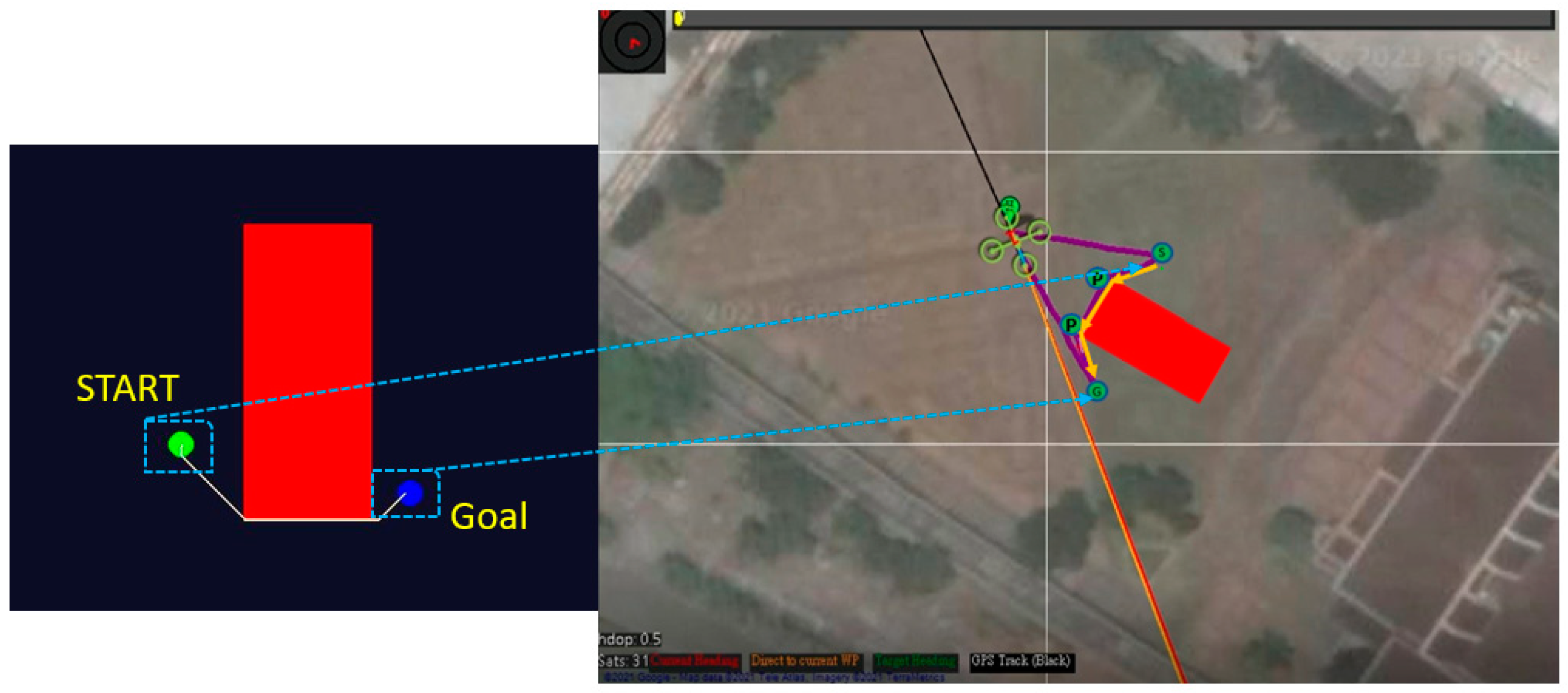
In Experiment 2, the no-fly zone was increased into two areas, shown as the red square and rectangle in Figure 32. The enlarged working area is shown in the left-hand figure of Figure 32. The planned path is the yellow line, which is indicated in the left-hand figure of Figure 32. The UAV follows the converted latitude and longitude coordinates, which are the green points marked in the right-hand figure of Figure 32 for the path of flight.
5.2. Obstacle Avoidance
The hexacopter’s front obstacle avoidance method is demonstrated using the Microsoft AirSim simulation software environment. In this simulation environment, many trees are placed as imaginary as sails on the sea, and there are undulations given to the terrain to simulate the waves on the sea. The drone continues to fly around in the virtual environment until it collides with an object.
In this simulation flight test, the input of the photo is 320 × 180 in size; the parameters are shown in Table 4. The number of training iterations was set to 140,000. We set the batch size to 32. If the batch size is increased, the convergence speed can be accelerated, but the hardware memory will not be able to load the data. The discount factor, γ, was set to 0.95, and the learning rate, α, was set to 0.000006. The smaller the learning rate is, the slower the convergence speed is.
In the training process, if the number of training times exceeds 150,000, the loss function will start to diverge, and the training effect will worsen. The loss function graph is shown in Figure 33.
After many iterations, the Q-value gradually increases to achieve the overall maximum benefit, as shown in Figure 34.
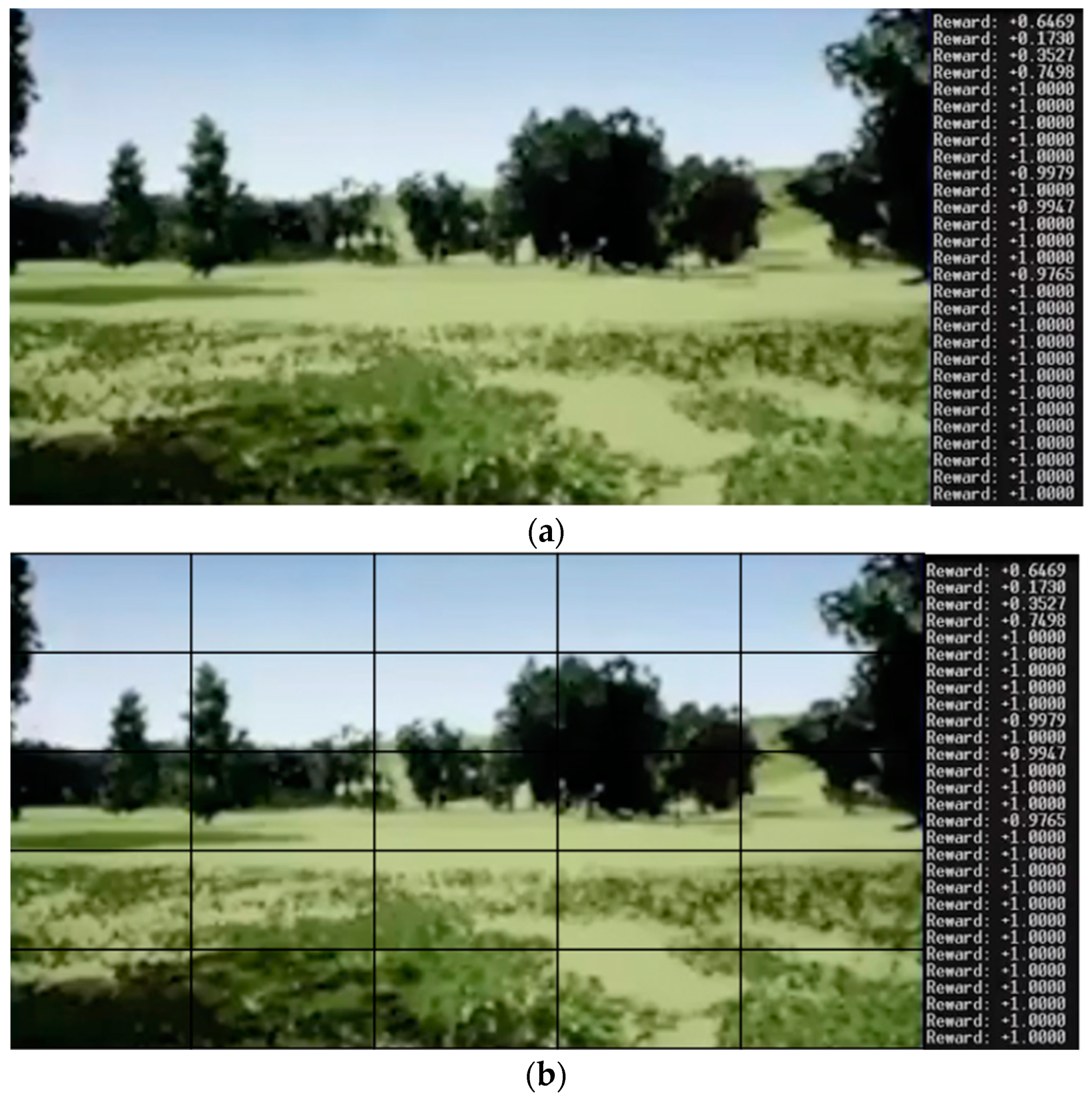
In the previous section, we mentioned a table with a 5 × 5 action space. The task of combining the action space with the input image is shown in Figure 35. There are mostly empty blocks placed in front of the drone; therefore, the rewards are continuously set to achieve the maximum score of +1. In terms of rewards, the scores are based on the proportion of colors in the pixels in the processed depth image, as shown in Figure 36.
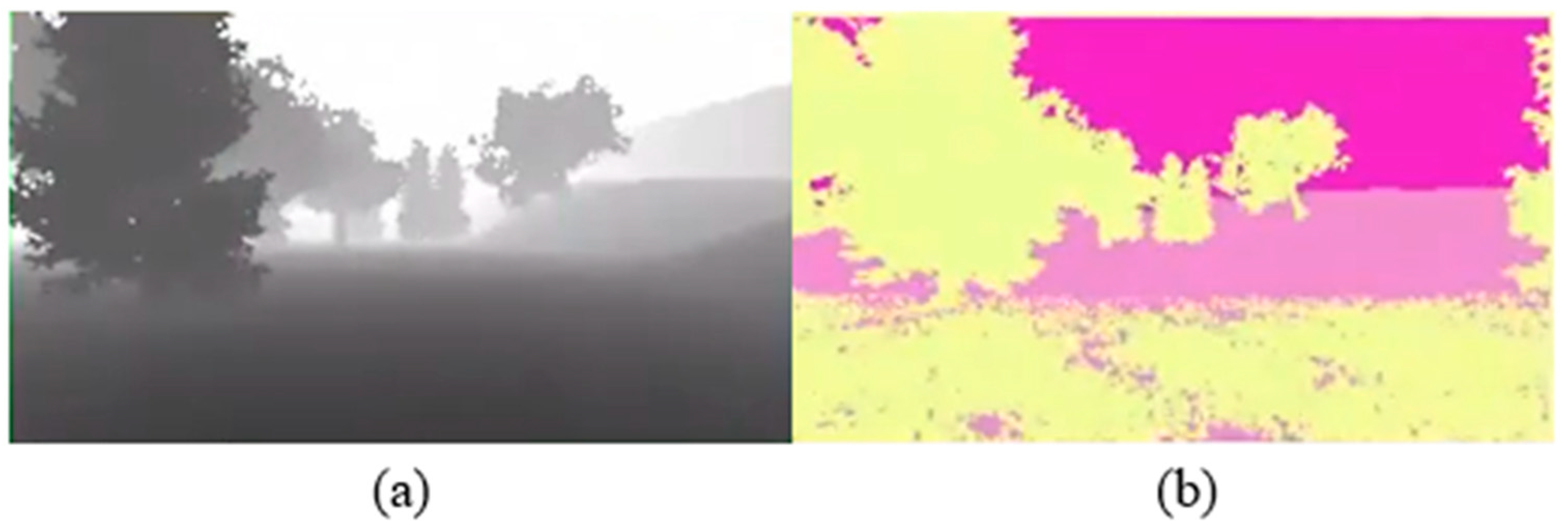
Figure 37 shows a scene full of trees and undulating terrain. Figure 38a is the first-person-view (FPV) depth image of the drone in Figure 37, while Figure 38b is the processed depth image and the yellow part represents proximity, so that the distances can be displayed more clearly.
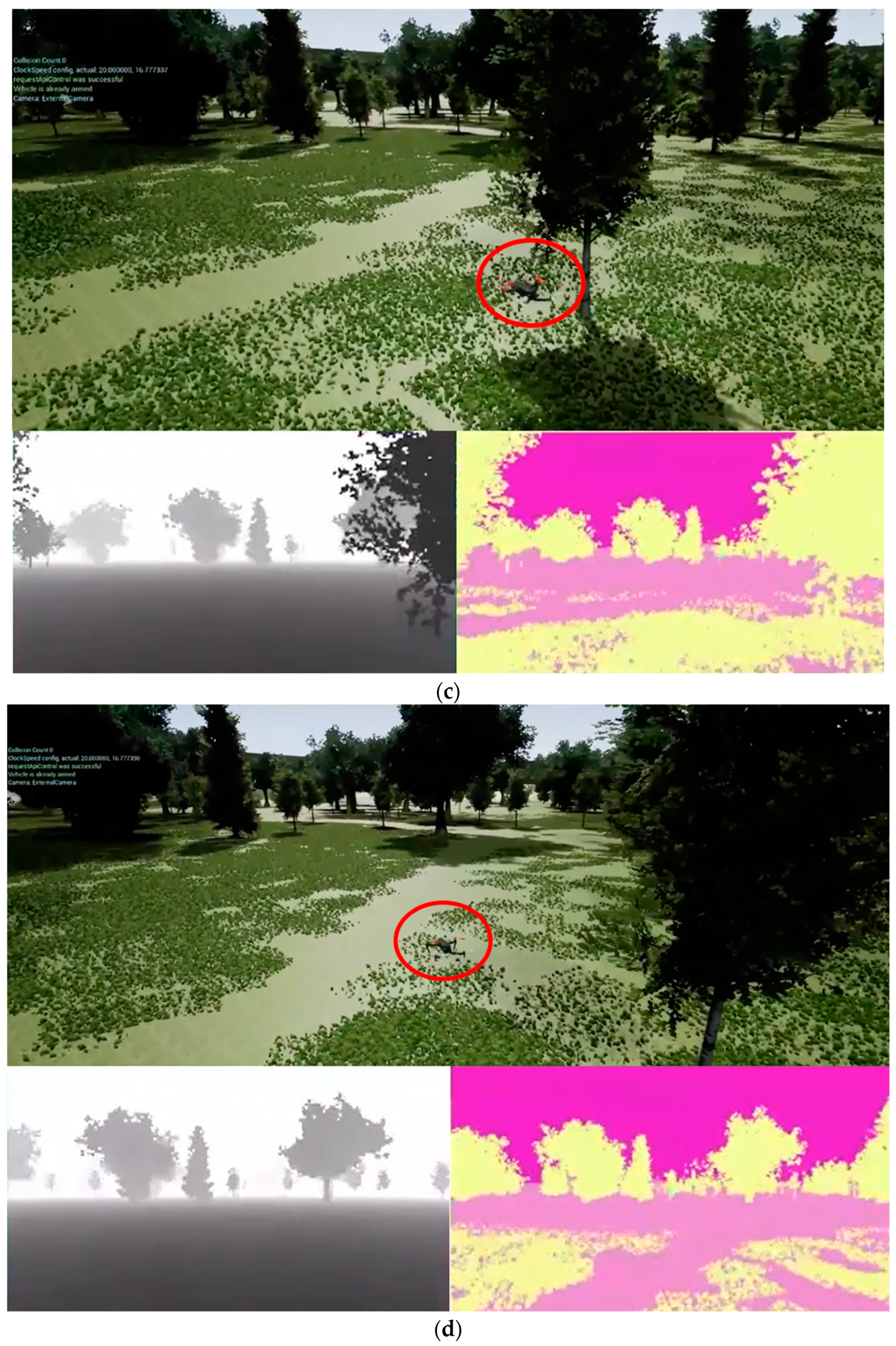
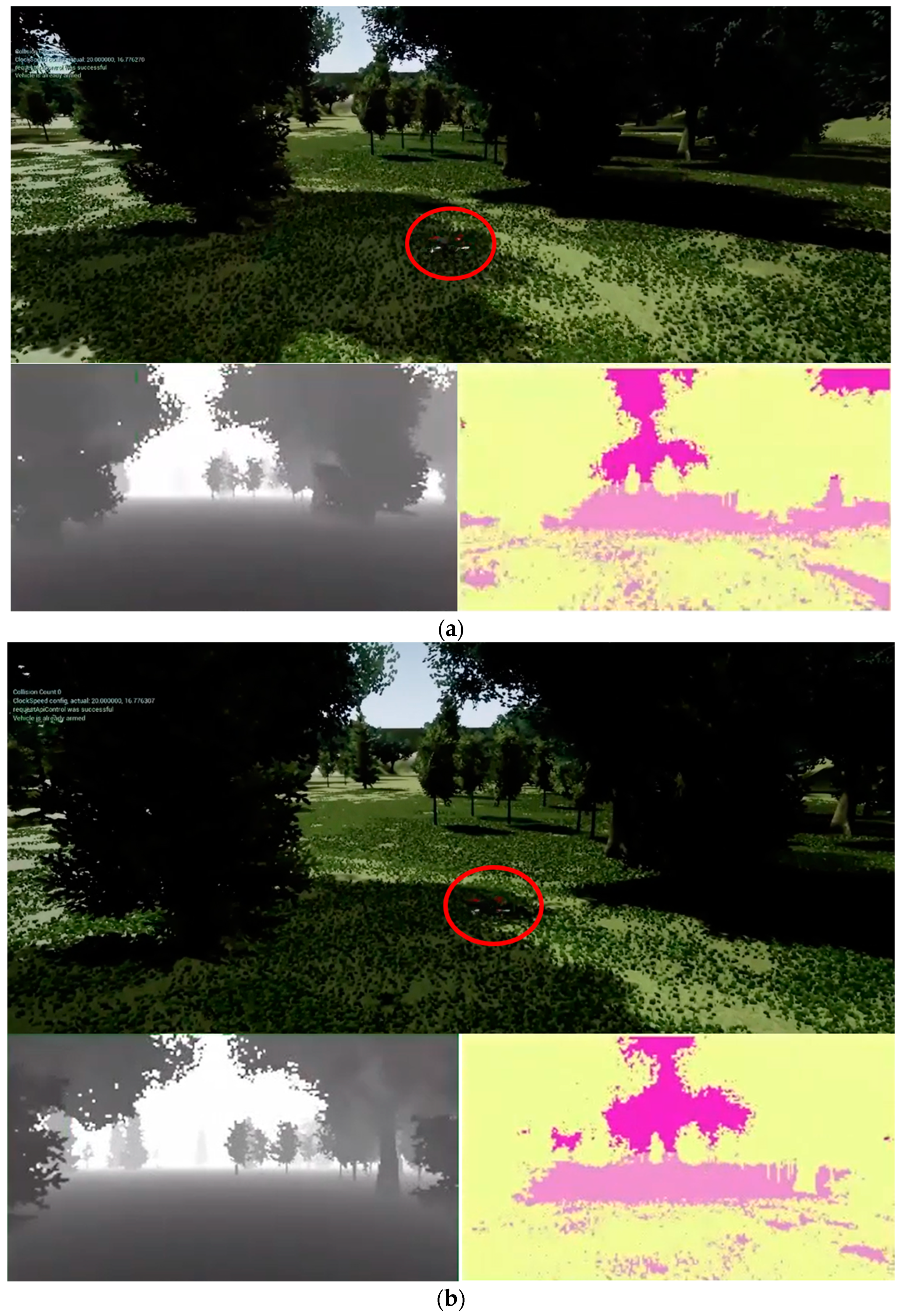
At this point, there is a tree directly in front of the drone. The drone sees the tree, as shown in Figure 39a, from a distance, and then starts to select the left-hand direction, based on the Q-table that has been trained. Figure 39b shows that the drone changes direction and the tree is unobstructed in front of the drone. Figure 39c shows the tree that was originally blocking the front of the drone but is now on the right-hand side of the drone. Finally, the UAV completely bypassed the obstacle, as shown in Figure 39d.
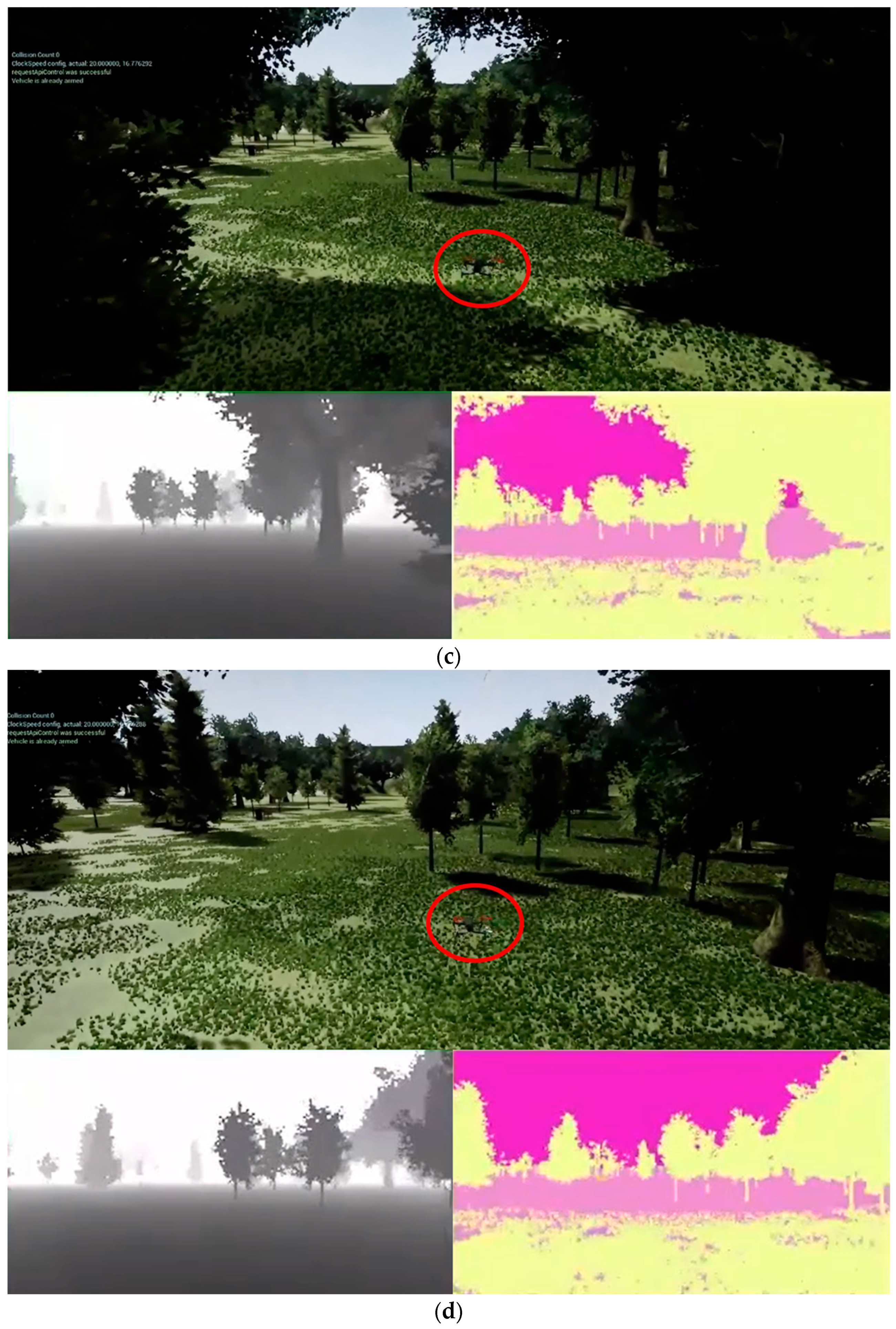
In the second test, there are two dense trees positioned in front of the drone. It can be seen from the depth map that the two trees can be passed between, as shown in Figure 40a. As the drone moves closer to the trees, it can be seen that the gap in the middle is wide enough to pass through, as shown in Figure 40b. During the crossing, the drone does not fly in a straight line. As shown in Figure 40c, the direction of the UAV is slightly offset, but afterward, the path has been adjusted to the open area. Finally, the UAV has successfully passed through the obstacles, as shown in Figure 40d.
The experiments show that the improved Q-learning algorithm, with the use of new reward and Q-value-updating rules, shows better performance in path planning than the classical reinforcement learning algorithm, SARSA. When we compare the improved Q-learning algorithm with the SARSA algorithm, the improved Q-learning algorithm can reduce computation time by 50% and shorten the path length by 30%. In terms of obstacle avoidance, the proposed deep-learning neural network with deep Q-learning can provide discrete action selections to enable UAVs to avoid obstacles. Real-time visual collision avoidance can be performed successfully. In addition, the proposed ultrasound obstacle avoidance method can achieve a distance error of less than 1.5% and a computing time of less than 0.2 s.
6. Conclusions
Research studies into UAVs have been booming in the past few years, and the methods of reinforcement learning also present a relatively challenging research field. This paper mainly focuses on the flight processes of UAVs, with a research background of dropping sensors from land to the net-cages used in sea-farming. In this study, UAV path planning using Q-learning and SARSA are placed under new reward and punishment rules, and the Q value updating rules are changed. The results for these two reinforcement learning algorithms are compared. In the real world, the coordinates are converted into latitude and longitude positions and the actual flight route. Using reinforcement learning methods to train UAVs in the real world will be expensive in terms of UAV cost consumption. Therefore, we chose to conduct our research in a virtual environment. The suggested obstacle avoidance method uses a deep Q-learning network (DQN) with an appropriate learning rate, batch size, and iteration, subsequently observing the obstacle-dodging results after training. Depth images from the UAV comprise the inputs of the DQN. The DQN provides discrete action selections for the UAV to avoid obstacles. Real-time visual collision avoidance can thus be performed. For dynamic obstacles to the side of the drone (out of sight), ultrasonic sensors are used; then, the sensing signals are filtered to maintain a stable sensing distance and to adjust UAV displacement after detecting the obstacle. Since drones are susceptible to airflow changes in the external environment and this can affect the fineness of flight, we used a simple control method that maintained a safe distance from objects to ensure that the UAV stayed away from the obstacles.
Path planning and obstacle avoidance are very important and basic functions for UAVs. The use of the Q-learning algorithm, a reinforcement learning method, can solve many of the complex problems that traditional algorithms cannot solve; therefore, there is plenty of room for development in the field of artificial intelligence. In this study, a Q-learning algorithm is proposed for application to path planning in an unknown environment. In terms of path planning, the reward design and action selection in the SARSA algorithm and Q-learning algorithm are similar to the methods of real-world learning. In terms of updating the Q-table, it is obvious that the Q-learning algorithm offers better benefits because the benefits of the overall path are considered fully. When we compared the modified Q-learning algorithm with the SARSA algorithm, the modified Q-learning algorithm showed better performance by reducing computation time by 50% and path length by 30%. In terms of obstacle avoidance, the application of UAV dodging is presented. Deep learning, when combined with reinforcement learning, can solve many complex problems, and obstacle avoidance is indeed a complex problem. The design method of experience replay allows the drone to access past states and actions that are similar to deep learning methods, which generally provide a label for learning. The side of the drone used for ultrasonic sensing obstacle avoidance will also effectively keep the drone at a safe distance from approaching objects. The proposed obstacle avoidance method can achieve a distance error of less than 1.5% and a computing time of less than 0.2 sec. For path planning and obstacle avoidance in more complex environments, reinforcement learning is expected to show further amazing results; there is no standard answer to this method, therefore the results will be different each time, and this is expected to enable even more amazing results. The main limitation of this work is the obstacle avoidance distance. The proposed system utilizes ultrasonic sensors to measure the distance between the UAV and the obstacles, but the measuring distance is short. In the case of high-speed moving objects, the UAV does not have enough time for computing a path and avoiding dynamic obstacles. In the future, a laser detector with a long measurement range will be needed to replace the ultrasonic sensors.
Author Contributions
Conceptualization, G.-T.T. and J.-G.J.; methodology, G.-T.T. and J.-G.J.; software, G.-T.T.; validation, G.-T.T. and J.-G.J.; formal analysis, G.-T.T. and J.-G.J.; investigation, G.-T.T. and J.-G.J.; resources, G.-T.T. and J.-G.J.; data curation, G.-T.T.; writing—original draft preparation, G.-T.T.; writing—review and editing, J.-G.J.; visualization, G.-T.T. and J.-G.J.; supervision, J.-G.J.; project administration, J.-G.J.; funding acquisition, J.-G.J. All authors have read and agreed to the published version of the manuscript.
Funding
This research was funded by Ministry of Science and Technology (Taiwan), grant number MOST 110-2221-E-019-075-MY2.
Institutional Review Board Statement
Not applicable.
Informed Consent Statement
Not applicable.
Data Availability Statement
Not applicable.
Conflicts of Interest
The authors declare no conflict of interest.
References
- Hart, P.E.; Nilsson, N.J.; Raphael, B. A formal basis for the heuristic determination of minimum cost paths. IEEE Trans. Syst. Sci. Cybern. 1968, 4, 100–107. [Google Scholar] [CrossRef]
- Stentz, A. Optimal and efficient path planning for unknown and dynamic environments. Int. J. Robot. Autom. Syst. 1995, 10, 89–100. [Google Scholar]
- LaValle, S.M.; Kuffner, J.J. Randomized kinodynamic planning. Int. J. Robot. Res. 2001, 20, 378–400. [Google Scholar] [CrossRef]
- Sen, Y.; Zhongsheng, W. Quad-Rotor UAV Control Method Based on PID Control Law. In Proceedings of the 2017 International Conference on Computer Network, Electronic and Automation (ICCNEA), Xi’an, China, 23–26 September 2017; pp. 418–421. [Google Scholar] [CrossRef]
- Kamel, B.; Yasmina, B.; Laredj, B.; Benaoumeur, I.; Zoubir, A. Dynamic Modeling, Simulation and PID Controller of Unmanned Aerial Vehicle UAV. In Proceedings of the 2017 Seventh International Conference on Innovative Computing Technology (INTECH), Porto, Portugal, 12–13 July 2017; pp. 64–69. [Google Scholar] [CrossRef]
- Lee, S.; Shim, T.; Kim, S.; Park, J.; Hong, K.; Bang, H. Vision-Based Autonomous Landing of a Multi-Copter Unmanned Aerial Vehicle using Reinforcement Learning. In Proceedings of the 2018 International Conference on Unmanned Aircraft Systems (ICUAS), Dallas, TX, USA, 12–15 June 2018; pp. 108–114. [Google Scholar] [CrossRef]
- Sugimoto, T.; Gouko, M. Acquisition of Hovering by Actual UAV Using Reinforcement Learning. In Proceedings of the 2016 3rd International Conference on Information Science and Control Engineering (ICISCE), Beijing, China, 8–10 July 2016; pp. 148–152. [Google Scholar] [CrossRef]
- Lampersberger, T.; Feger, R.; Haderer, A.; Egger, C.; Friedl, M.; Stelzer, A. A 24-GHz Radar with 3D-Printed and Metallized Lightweight Antennas for UAV Applications. In Proceedings of the 2018 48th European Microwave Conference (EuMC), Madrid, Spain, 23–27 September 2018; pp. 1413–1416. [Google Scholar] [CrossRef]
- Udvardy, P.; Jancsó, T.; Beszédes, B. 3D Modelling by UAV Survey in a Church. In 2019 New Trends in Aviation Development (NTAD); IEEE: Piscataway, NJ, USA, 2019; pp. 189–192. [Google Scholar] [CrossRef]
- Ma, Z.; Ai, B.; He, R.; Wang, G.; Niu, Y.; Zhong, Z. A Wideband Non-Stationary Air-to-Air Channel Model for UAV Communications. IEEE Trans. Veh. Technol. 2020, 69, 1214–1226. [Google Scholar] [CrossRef]
- Feng, K.; Li, W.; Ge, S.; Pan, F. Packages Delivery Based on Marker Detection for UAVs. In Proceedings of the 2020 Chinese Control and Decision Conference (CCDC), Hefei, China, 22–24 August 2020; pp. 2094–2099. [Google Scholar] [CrossRef]
- Silver, D.; Huang, A.; Maddison, C.J.; Guez, A.; Sifre, L.; Van Den Driessche, G.; Schrittwieser, J.; Antonoglou, I.; Panneershelvam, V.; Lanctot, M.; et al. Mastering the Game of Go with Deep Neural Networks and Tree Search. Nature 2016, 529, 484–489. [Google Scholar] [CrossRef] [PubMed]
- Yan, C.; Xiang, X. A Path Planning Algorithm for UAV Based on Improved Q-Learning. In Proceedings of the 2018 2nd International Conference on Robotics and Automation Sciences (ICRAS), Wuhan, China, 23–25 June 2018; pp. 1–5. [Google Scholar] [CrossRef]
- Zhang, T.; Huo, X.; Chen, S.; Yang, B.; Zhang, G. Hybrid Path Planning of a Quadrotor UAV Based on Q-Learning Algorithm. In Proceedings of the 2018 37th Chinese Control Conference (CCC), Wuhan, China, 25–27 July 2018; pp. 5415–5419. [Google Scholar] [CrossRef]
- Li, R.; Fu, L.; Wang, L.; Hu, X. Improved Q-learning Based Route Planning Method for UAVs in Unknown Environment. In Proceedings of the 2019 IEEE 15th International Conference on Control and Automation (ICCA), Edinburgh, UK, 16–19 July 2019; pp. 118–123. [Google Scholar] [CrossRef]
- Hou, X.; Liu, F.; Wang, R.; Yu, Y. A UAV Dynamic Path Planning Algorithm. In Proceedings of the 2020 35th Youth Academic Annual Conference of Chinese Association of Automation (YAC), Zhanjiang, China, 16–18 October 2020; pp. 127–131. [Google Scholar] [CrossRef]
- Anwar, A.; Raychowdhury, A. Autonomous Navigation via Deep Reinforcement Learning for Resource Constraint Edge Nodes Using Transfer Learning. IEEE Access 2020, 8, 26549–26560. [Google Scholar] [CrossRef]
- Singla, A.; Padakandla, S.; Bhatnagar, S. Memory-Based Deep Reinforcement Learning for Obstacle Avoidance in UAV With Limited Environment Knowledge. IEEE Trans. Intell. Transp. Syst. 2021, 22, 107–118. [Google Scholar] [CrossRef]
- Duc, N.; Hai, Q.; Van, D.; Trong, T.; Trong, T. An Approach for UAV Indoor Obstacle Avoidance Based on AI Technique with Ensemble of ResNet8 and Res-DQN. In Proceedings of the 2019 6th NAFOSTED Conference on Information and Computer Science (NICS); 2019; pp. 330–335. [Google Scholar] [CrossRef]
- Çetin, E.; Barrado, C.; Muñoz, G.; Macias, M.; Pastor, E. Drone Navigation and Avoidance of Obstacles Through Deep Reinforcement Learning. In Proceedings of the 2019 IEEE/AIAA 38th Digital Avionics Systems Conference (DASC), San Diego, CA, USA, 8–12 September 2019; pp. 1–7. [Google Scholar] [CrossRef]
- Wu, T.; Tseng, S.; Lai, C.; Ho, C.; Lai, Y. Navigating Assistance System for Quadcopter with Deep Reinforcement Learning. In Proceedings of the 2018 1st International Cognitive Cities Conference (IC3), Okinawa, Japan, 7–9 August 2018; pp. 16–19. [Google Scholar] [CrossRef]
- Tu, G.; Juang, J. Path Planning and Obstacle Avoidance Based on Reinforcement Learning for UAV Application. In Proceedings of the 2021 International Conference on System Science and Engineering, Ho Chi Minh City, Vietnam, 26–28 August 2021. [Google Scholar]
- Zheng, Y.; Wang, L.; Xi, P. Improved Ant Colony Algorithm for Multi-Agent Path Planning in Dynamic Environment. In Proceedings of the 2018 International Conference on Sensing, Diagnostics, Prognostics, and Control (SDPC), Xi’an, China, 15–17 August 2018; pp. 732–737. [Google Scholar] [CrossRef]
- Zhang, D.; Xian, Y.; Li, J.; Lei, G.; Chang, Y. UAV Path Planning Based on Chaos Ant Colony Algorithm. In Proceedings of the 2015 International Conference on Computer Science and Mechanical Automation (CSMA), Washington, DC, USA, 23–25 October 2015; pp. 81–85. [Google Scholar] [CrossRef]
- Yujie, L.; Yu, P.; Yixin, S.; Huajun, Z.; Danhong, Z.; Yong, S. Ship Path Planning Based on Improved Particle Swarm Optimization. In Proceedings of the 2018 Chinese Automation Congress (CAC), Xi’an, China, 20 November–2 December 2018; pp. 226–230. [Google Scholar] [CrossRef]
- Markov, A.A. Extension of the Limit Theorems of Probability Theory to a Sum of Variables Connected in a Chain; Reprinted in Appendix B of: R. Howard. Dynamic Probabilistic Systems, Volume 1: Markov Chains; John Wiley and Sons: Hoboken, NJ, USA, 1971. [Google Scholar]
- Sammut, C.; Webb, G.I. (Eds.) Bellman Equation. In Encyclopedia of Machine Learning; Springer: Boston, MA, USA, 2011. [Google Scholar] [CrossRef]
- Cormen, T.H.; Leiserson, C.E.; Rivest, R.L.; Stein, C. 16 Greedy Algorithms. In Introduction to Algorithms; MIT Press: Cambridge, MA, USA, 2001; p. 370. ISBN 978-0-262-03293-3. [Google Scholar]
- Tokic, M. Adaptive ε-greedy Exploration in Reinforcement Learning Based on Value Differences. In KI 2010: Advances in Artificial Intelligence; Lecture Notes in Computer Science, 6359; Springer-Verlag: Berlin/Heidelberg, Germany, 2010; pp. 203–210. [Google Scholar] [CrossRef] [Green Version]
- Watkins, C.; Dayan, P. Q-learning. Mach. Learn. 1992, 8, 279–292. [Google Scholar] [CrossRef]
- Xu, D.; Fang, Y.; Zhang, Z.; Meng, Y. Path Planning Method Combining Depth Learning and Sarsa Algorithm. In Proceedings of the 2017 10th International Symposium on Computational Intelligence and Design (ISCID), Hangzhou, China, 9–10 December 2017; pp. 77–82. [Google Scholar] [CrossRef]
- Zhou, B.; Wang, W.; Wang, Z.; Ding, B. Neural Q Learning Algorithm based UAV Obstacle Avoidance. In Proceedings of the 2018 IEEE CSAA Guidance, Navigation and Control Conference (CGNCC), Xiamen, China, 10–12 August 2018; pp. 1–6. [Google Scholar] [CrossRef]
- Xiaodong, Y.; Rui, L.; Yingjing, S.; Xiang, C. Obstacle Avoidance for Outdoor Flight of a Quadrotor Based on Computer Vision. In Proceedings of the 2017 29th Chinese Control and Decision Conference (CCDC), Chongqing, China, 28–30 May 2017; pp. 3841–3846. [Google Scholar] [CrossRef]
- Hu, J.; Niu, Y.; Wang, Z. Obstacle Avoidance Methods for Rotor UAVs Using RealSense Camera. In Proceedings of the 2017 Chinese Automation Congress (CAC); 2017; pp. 7151–7155. [Google Scholar] [CrossRef]
- Mnih, V.; Kavukcuoglu, K.; Silver, D.; Graves, A.; Antonoglou, I.; Wierstra, D.; Riedmiller, M. Playing Atari with Deep Reinforcement Learning. arXiv 2013, arXiv:1312.5602. [Google Scholar]
- Airsim Open Source Platform at Github. Available online: https://github.com/Microsoft/AirSim (accessed on 23 July 2020).
- Huang, T.; Juang, J. Real-time Path Planning and Fuzzy Based Obstacle Avoidance for UAV Application. In Proceedings of the 2020 International Conference on System Science and Engineering (ICSSE), Kagawa, Japan, 31 August–3 September 2020. [Google Scholar]
Figure 1.
UAV system structure.

Figure 2.
RTK ground station.

Figure 3.
Working procedure of the proposed approach.

Figure 4.
The hexacopter setup.

Figure 5.
The interaction between the agent and the environment.

Figure 6.
Example of the calculation of value function.

Figure 7.
Operation of the greedy policy.

Figure 8.
Operation of the - greedy policy.

Figure 9.
Q-learning algorithm procedure.

Figure 10.
Flowchart of the Q-learning algorithm.

Figure 11.
The schematic diagram of the reward and punishment rules.

Figure 12.
The routes in the reward and punishment rules.

Figure 13.
Grid map stored in a Q-table.

Figure 14.
The SARSA algorithm procedure.

Figure 15.
Example in the grid-world environment.

Figure 16.
The SARSA algorithm route.

Figure 17.
The Q-learning algorithm route.

Figure 18.
Interaction between the DQN and the environment.

Figure 19.
The DQN algorithm diagram.

Figure 20.
AirSim environment screenshot.

Figure 21.
DQL obstacle avoidance flow chart.

Figure 22.
Network architecture.

Figure 23.
The 5 × 5 action space.

Figure 24.
Illustration of the ultrasonic process.

Figure 25.
The experiment in Environment 1: (a) SARSA algorithm, (b) Q-learning algorithm.

Figure 26.
Training results of Q-Learning and SARSA in Environment 1, (a) is Q-Learning training result, (b) is SARSA training result.
Figure 26.
Training results of Q-Learning and SARSA in Environment 1, (a) is Q-Learning training result, (b) is SARSA training result.

Figure 27.
The Q-table for Q-learning and SARSA in Environment 1.

Figure 28.
The experiment in Environment 2: (a) SARSA algorithm, (b) Q-learning algorithm.

Figure 29.
Training results of Q-learning and SARSA in Environment 2.

Figure 30.
The Q-table of Q-learning and SARSA in Environment 2.

Figure 31.
The Q-learning path on the map for Experiment 1.

Figure 32.
The Q-learning path on the map in Experiment 2.

Figure 33.
The graph showing the loss function.

Figure 34.
The maximum Q-value.

Figure 35.
The first-person views of the drone and the rewards, next to: (a) the original RGB image, (b) the same image, divided into a 5 × 5 action space.
Figure 35.
The first-person views of the drone and the rewards, next to: (a) the original RGB image, (b) the same image, divided into a 5 × 5 action space.

Figure 36.
The depth image, divided into a 5 × 5 action space. (a) The original depth image. (b) The processed depth image.
Figure 36.
The depth image, divided into a 5 × 5 action space. (a) The original depth image. (b) The processed depth image.

Figure 37.
A scene full of trees and undulating terrain.

Figure 38.
The depth image from Figure 37, (a) is the first-person-view depth image of the drone in Figure 37, (b) is the processed depth image.

Figure 39.
The experiment for testing obstacle avoidance in the simulation environment (part 1), (a) is the starting point, (b) shows the drone changes direction, (c) shows the tree is now on the right-hand side of the drone, (d) shows the UAV completely bypassed the obstacle.
Figure 39.
The experiment for testing obstacle avoidance in the simulation environment (part 1), (a) is the starting point, (b) shows the drone changes direction, (c) shows the tree is now on the right-hand side of the drone, (d) shows the UAV completely bypassed the obstacle.


Figure 40.
The experiment for testing obstacle avoidance in the simulation environment, part 2, (a) is the starting point, (b) shows the drone moves closer to the trees, (c) shows the drone does not fly in a straight line, (d) shows the UAV has successfully passed through the obstacles.
Figure 40.
The experiment for testing obstacle avoidance in the simulation environment, part 2, (a) is the starting point, (b) shows the drone moves closer to the trees, (c) shows the drone does not fly in a straight line, (d) shows the UAV has successfully passed through the obstacles.


Table 1.
The HC-SR04 sensor, with a filter test.
| Error (cm) | Error Percentage | Cost Time (s) | ||
|---|---|---|---|---|
| 35 | 34.97 | 0.03 | 0.08% | 0.0205 |
| 60 | 59.88 | 0.12 | 0.20% | 0.0311 |
| 75 | 75.69 | 0.69 | 0.92% | 0.0363 |
| 100 | 100.45 | 0.45 | 0.45% | 0.0429 |
| 200 | 198.79 | 1.21 | 0.605% | 0.0812 |
| 250 | 246.42 | 3.58 | 1.432% | 0.0965 |
| 300 | 297.28 | 2.72 | 0.906% | 0.1203 |
| 350 | 346.58 | 3.42 | 0.977% | 0.1299 |
| 400 | 394.56 | 5.44 | 1.36% | 0.1483 |
| 450 | 443.42 | 6.58 | 1.462% | 0.1712 |
Table 2.
The results compared for Environment 1.
| Environment 1 | SARSA | Q-Learning |
|---|---|---|
| path length | 62 steps | 42 steps |
| exploration time | 32 min | 15 min |
Table 3.
The results compared for Environment 2.
| Environment 2 | SARSA | Q-Learning |
|---|---|---|
| path length | 140 steps | 46 steps |
| exploration time | 45 min | 25 min |
Table 4.
Training parameters.
| Iterations | Batch Size | ||
|---|---|---|---|
| 140,000 | 32 | 0.95 | 0.000006 |
Disclaimer/Publisher’s Note: The statements, opinions and data contained in all publications are solely those of the individual author(s) and contributor(s) and not of MDPI and/or the editor(s). MDPI and/or the editor(s) disclaim responsibility for any injury to people or property resulting from any ideas, methods, instructions or products referred to in the content. |
© 2023 by the authors. Licensee MDPI, Basel, Switzerland. This article is an open access article distributed under the terms and conditions of the Creative Commons Attribution (CC BY) license (https://creativecommons.org/licenses/by/4.0/).
Share and Cite
MDPI and ACS Style
Tu, G.-T.; Juang, J.-G. UAV Path Planning and Obstacle Avoidance Based on Reinforcement Learning in 3D Environments. Actuators 2023, 12, 57. https://doi.org/10.3390/act12020057
AMA Style
Tu G-T, Juang J-G. UAV Path Planning and Obstacle Avoidance Based on Reinforcement Learning in 3D Environments. Actuators. 2023; 12(2):57. https://doi.org/10.3390/act12020057
Chicago/Turabian StyleTu, Guan-Ting, and Jih-Gau Juang. 2023. "UAV Path Planning and Obstacle Avoidance Based on Reinforcement Learning in 3D Environments" Actuators 12, no. 2: 57. https://doi.org/10.3390/act12020057
Note that from the first issue of 2016, this journal uses article numbers instead of page numbers. See further details here.