A Double-Layer Model Predictive Control Approach for Collision-Free Lane Tracking of On-Road Autonomous Vehicles

Abstract

This paper proposes a double-layer model predictive control (MPC) algorithm for the integrated path planning and trajectory tracking of autonomous vehicles on roads. The upper module is responsible for generating collision-free lane trajectories, while the lower module is responsible for tracking this trajectory. A simplified vehicle model based on the friction cone is proposed to reduce the computation time for trajectory planning in the upper layer module. To achieve dynamic and accurate collision avoidance, a polygonal distance-based dynamic obstacle avoidance method is proposed. A vertical load calculation method for the tires is introduced to design the anti-rollover constraint in the lower layer module. Numerical simulations, with static and dynamic obstacle scenarios, are conducted on the MATLAB platform and compared with two state-of-the-art MPC algorithms. The results demonstrate that the proposed algorithm outperforms the other two algorithms regarding computation time and collision avoidance efficiency.

1. Introduction

Autonomous driving is a rapidly developing field with promising prospects for enhancing road safety, reducing traffic congestion, and improving transportation efficiency [1]. However, the safety factor remains a critical bottleneck, as autonomous vehicles must operate safely in complex and unpredictable traffic environments. Moreover, ensuring precise trajectory planning and tracking is essential to achieving efficient and stable vehicle control. To address these challenges, researchers have proposed various approaches, including MPC-based techniques, which have demonstrated significant potential in enhancing both safety and control accuracy. Nevertheless, further research is necessary to optimize the performance of MPC-based methods for real-world autonomous driving applications.

The recent advancements in computing technology have brought significant attention to the MPC algorithm in the field of autonomous driving. Unlike traditional feedback control algorithms, the MPC algorithm has the capability to address both the constraints of state variables and input variables, as well as to predict the future state of the system and determine the necessary inputs to minimize a pre-defined cost function. This architecture is particularly suitable for autonomous driving technology, as the control of autonomous vehicles requires consideration of not only the physical restrictions of actuators, but also various constraints such as traffic regulations, collision avoidance requirements, safety regulations, and other relevant factors [2].

The implementation of MPC-based autonomous vehicle control techniques involves the selection of an appropriate vehicle dynamics model. The extensive study of full vehicle dynamics models, from tire models to high-fidelity models, highlights the need for a balance between model accuracy and computational time. A 14-degree-of-freedom (14-DOF) high-precision model has been proposed in [3], which incorporates detailed handling, ride, and tire models. The results of experiments conducted on an instrumented experimental vehicle demonstrate the capability of the model to accurately predict the state of the vehicle. However, while the high-fidelity model offers a precise prediction of the evolution of the vehicle state, its computational demands result in limited prediction lengths. In the case of shorter prediction intervals, the requirement for an obstacle avoidance response within a short time frame is not conducive to safe vehicle operation [4]. As a result, various model selection schemes for MPC controllers have been investigated. The authors of [5] have verified the feasibility of 2-DOF and 3-DOF vehicle models, with experimental results indicating that a 2-degree-of-freedom vehicle model with a linear tire model is sufficient for collision avoidance in static obstacle scenarios. Furthermore, the authors of [6] have shown that an 8-degree-of-freedom vehicle model with successive linearization is appropriate for LVP-MPC and is capable of achieving high-performance trajectory tracking.

The use of MPC in autonomous vehicles has demonstrated the ability to accurately track a specified trajectory in obstacle-free environments. However, the presence of road traffic poses a collision avoidance challenge, leading to the introduction of non-convex and non-smooth constraints in the MPC algorithm, thereby complicating its solution. Collision-free trajectory tracking is a crucial requirement for the practical implementation of autonomous vehicles. In response to this challenge, a previous study [7] has proposed a collision avoidance algorithm based on a center point-based model, which represents the vehicle as a rectangle and computes the safe distance between vehicles using the geometric center point. This method simplifies the collision avoidance constraint to a smooth quadratic constraint, thus facilitating the solution. Although this method has shown effectiveness in broad driving environments, it may not be suitable for narrow areas, such as overtaking lanes, where inter-vehicle distances are limited. To address this issue, a mixed integer linear programming-based collision avoidance algorithm, with semidefinite planning, has been proposed to ensure real-time performance [8]. While these methods handle static obstacles, they do not consider collision avoidance among dynamic vehicles in complex road traffic environments. Another study [9] proposed using spatial coordinate changes to simplify the motion model of moving vehicles to achieve moving obstacle collision avoidance.

Autonomous vehicle driving safety is a critical aspect of driverless technology that goes beyond simply avoiding collisions. The authors of [10] indicate that for an autonomous vehicle to maintain a safe and stable tracking path under conditions of reduced friction, the estimation error of tire friction must be no less than 2%. As the current estimation accuracy is insufficient, a slip angle-based control strategy is proposed to maintain the front wheel friction within the maximum friction range at all times. Another study develops a rollover prediction algorithm based on the dynamic load transfer rate and demonstrates through practical experiments that rollover can be effectively prevented by restricting the steering angle [11]. Several vehicle safety control algorithms for various limit cases are proposed in the literature [12,13,14]. The authors of [12] proposed an integrated controller using the collaborative control of 4WS and tube-based MPC to improve the handling stability and path-tracking performance of automated electric vehicles at driving limits. However, the main limitation of tube-based MPC is the conservative strategy planned by the robust principle, which may limit the performance of the system. The authors of [13] proposed a high-fidelity nonlinear MPC algorithm that considers vehicle rollover constraints to ensure rapid completion of missions in field environments. Due to the nonlinear characteristics of the vehicle, the computation time of the single-layer nonlinear model predictive control (NMPC) algorithm is too long, and this approach needs further optimization in urban traffic environments. The authors of [14] proposed a hierarchical MPC structure to reduce the computational complexity of trajectory tracking under non-ideal road conditions. However, the oversimplified point-mass model cannot guarantee that the vehicle is free from rollover risks.

The stability and real-time performance of MPC algorithms are obstacles that have been encountered in the field. To address the stability issue, the author of [15] has employed invariant set theory to guarantee the persistence feasibility of the system’s initial state. However, for complex optimization problems with security constraints and nonlinear tire dynamics, a systematic approach to proving the stability of MPC algorithms has yet to be established. To address the real-time performance, the authors of [16] have proposed real-time MPC-based trajectory tracking for autonomous vehicles, with a computational cycle of MPC that can be completed at a 20 Hz sampling frequency. However, the complexity of the nonlinear algorithm limits the real-time MPC algorithm to low vehicle speeds and favorable road conditions [17].

Based on the literature review, it has been identified that there exists potential for further enhancement in MPC-based autonomous technology. While previous studies in [13,14] have proposed enhanced MPC algorithms to improve both the computational complexity and driving safety of autonomous vehicles, this paper builds upon these advancements by introducing additional improvements. Inspired by the studies in [13,14], the present paper introduces a triple novelty:

(1)

This paper proposes a novel double-layer structure MPC algorithm to achieve lane tracking for on-road autonomous vehicles. The double-layer structure separates the trajectory planning and tracking tasks. The upper layer module uses a simplified vehicle model to calculate collision-free trajectories in real-time, while the lower layer module uses a higher fidelity vehicle model to track the trajectory.

(2)

This paper proposes a simplified vehicle model based on the second-order norm friction cone in the upper layer. Introducing the second-order norm friction cone simplifies the trajectory planning difficulty while capturing the characteristics of tire friction. Furthermore, this paper proposes a polygonal distance-based dynamic obstacle avoidance method. The polygonal calculation formula calculates the distance between the ego vehicle and obstacles precisely, and neighboring vehicles’ states are augmented into the ego vehicle’s state space to plan the dynamic collision-free trajectory.

(3)

This paper introduces the calculation of the vertical load of tires to design the anti-rollover constraint in the lower layer, which represents the contact situation between tires and the ground. This constraint ensures that the vertical load of each tire is higher than the preset value to avoid rollover.

The remainder of the paper is structured as follows. Section 2 briefly introduces the basic principle of MPC and the method for selecting lane waypoints. Section 3 details the formulation of the double-layer structure MPC proposed in this paper, including vehicle model design, collision avoidance constraint design, and double-layer MPC structure design. Section 4 describes on-road autonomous vehicle trajectory tracking experiments with static and dynamic obstacles and compares them with the literature [13,14]. Section 5 concludes the paper.

2. Preliminaries

2.1. Model Predictive Control

Model predictive control is a control algorithm that is based on an optimization method. This approach differs from traditional control algorithms in its structure and places a greater emphasis on exploring the state space of the control object, as opposed to modifying its dynamics. The MPC algorithm has been shown to be more effective in specific control applications as a result of this difference [18].

The early use of MPC was primarily limited to the chemical industry, where it was applied to address regulation problems, also known as set point problems. At the time, the computational power available was a limiting factor in the application of MPC. However, with the advancements in computational science, MPC has now become a widely used technique in autonomous driving technology. This is due to its unique structure, which allows for the simulation of human driving behavior through the use of environmental information and vehicle dynamics. Additionally, MPC provides the ability to choose the optimal control strategy among multiple safety constraints, making it a highly useful tool in autonomous driving technology.

In the realm of control theory, MPC is a well-established approach to system control. When the system dynamics equations, constraints, and cost function are linear and affine, MPC is referred to as Linear MPC and can be solved using mature quadratic programming algorithms. The stability and optimization properties of Linear MPC have been widely studied. However, in the context of autonomous driving, Linear MPC may not achieve satisfactory performance due to the strong nonlinear characteristics of vehicle dynamics, safety constraints, and state constraints. To address this issue, NMPC has been developed as a variant of MPC. NMPC relaxes the convex constraints imposed by Linear MPC and addresses more general non-convex nonlinear constraints. This leads to the formulation of NMPC as a Nonlinear Programming problem.

The NMPC approach comprises two essential components: constraints and a cost function, and its formulation is described in Equation (1). At a particular sampling instance, t, the optimal solution minimizing the cost function over N prediction horizons is calculated, and this process is repeated at each subsequent sampling instance. For the implementation of feedback control, only the first control solution is utilized in each computation cycle, with subsequent computations being performed by shifting the prediction horizon forward.

The traditional single-layer MPC formulation design for autonomous vehicle driving consists of objectives and constraints. Equations (1) and (2) denotes a single-layer MPC formulation that involves the maneuver constraint, safety constraint, and predication distance constraint.

$$\begin{array}{l}\underset{u(·),x(·)}{\min }{\displaystyle {\sum }_{i=1}^{N-1}[Q_z(X(i|t)-X_{ref}(i|t))+}{Q}_u(u(i|t)-u_{ref}(i|t))]+\dots \\ Q_t(X(N|t)-X_{ref}(N|t))\end{array}$$

(1)

$$\begin{array}{ll}\hfill \mathrm{subject} \mathrm{to}& X(0|t)=X(t)\hfill \\ \hfill & X(i+1|t)=f_d(X(i|t),U(i|t))\hfill \\ \hfill & X_{\min }\le X(i|t)\le X_{\max }\hfill \\ \hfill & u_{\min }\le u(i|t)\le u_{\max }\hfill \\ \hfill & \begin{array}{l}safe\_dist\left(i\right|t)\le safety\_dist\\ pred\_dist(i|t)\le Visual\_threhold\end{array}\hfill \\ \hfill & F\_load(i|t)\le F\_threhold\hfill \\ \hfill & \forall i=0,\dots ,N;\forall k=1,\dots ,no\_obs\hfill \end{array}$$

(2)

According to Equation (1), the cost function serves to penalize deviations from reference vectors for both the state vector $X$ and the input vector $U$. The reference vectors for the state vector are the lane waypoints that are tracked by the autonomous vehicle, while the reference vectors for the input vector are zero vectors. This implies a desire for minimal input control efforts in order to conserve energy. The penalizing weighted positive definite matrices, $Q_Z$, $Q_u$, and $Q_t$, serve to assign appropriate weights to the deviation from the reference vectors.

The first two equations of Equation (2) are indicative of the requirement for the state variable $X$ to satisfy the dynamic equation of the system, such that the solution variable adheres to the physical principles governing the vehicle system. The third and fourth equations represent constraints on the state of the system and control input, as in the context of autonomous driving, the vehicle must maintain its position within the lane, and the control inputs (such as steering and throttle) are limited. The fifth equation serves as a collision avoidance constraint, ensuring that the vehicle avoids obstacles within its predicted horizon. The sixth equation requires that the predicted position remains within the effective range of the vision sensor, while the seventh equation imposes a safety constraint, requiring that the vertical load of each tire remains within a safe range to prevent rollover. Each constraint will be explained in detail, and its calculation formula will be presented in the following sections.

2.2. Lane Waypoint Selection

Lane tracking in autonomous vehicles refers to the capability of the vehicle to drive within a designated lane or follow a specified trajectory. The implementation of autonomous driving involves the use of several interconnected modules, including a top-down perception module, a decision-making module, a path-planning module, and a control module. The perception module provides the vehicle with relevant information about its surroundings, such as the environment’s image, the positioning of the vehicle, and obstacles. The decision-making module determines the actions to be taken by the vehicle, such as lane changes, overtaking, parking, and other driving behaviors. However, these two modules are outside the scope of this paper. The path planning module plans the vehicle’s path based on the decisions made by the decision-making module, resulting in a set of track points or trajectories. Finally, the control module ensures that the vehicle follows the planned trajectory by tracking it and making the necessary adjustments to the vehicle’s movement.

The process of lane tracking involves obtaining and interpolating highway waypoints from pre-existing map information. Map information is commonly stored on onboard equipment, and it is assumed in this paper that the lane waypoints have already been established. The vehicle can then calculate its distance from these waypoints. However, as the waypoints do not include time information and only provide positional information, it is necessary for the vehicle to select a reference waypoint in real-time in order to correct its position. The procedure for selecting reference waypoints is illustrated in Figure 1.

The position of COG of the vehicle at time t is represented by point $P\left(t\right)=[X\left(t\right),Y(t\left)\right]$, and its projections along the X-axis and Y-axis are denoted by $P_{ref\_x}\left(t\right)$ and $P_{ref\_y}\left(t\right)$, respectively. The reference point at any given moment is determined as the projection point closest to the goal. In Figure 1, for the purposes of this paper, $P_{ref\_y}$ is selected as the reference point. This approach not only simplifies the calculation of distance but also eliminates the issue of vehicles driving in the opposite direction that can arise from tracking the shortest distance point of a straight line. Because using the shortest distance of a straight line may result in a point in the opposite direction as a reference point.

The MPC utilizes predicted states to select N reference waypoints. During the sample time $t-1$, the MPC algorithm predicts N trajectory positions, $P\left(\Delta T\right|t-1),P(2\Delta T|t-1),\dots ,P\left(N\Delta T\right|t-1)$. These predicted trajectory positions are then utilized to generate N corresponding reference waypoints, $Pref\left(\Delta T\right|t-1),Pref(2\Delta T|t-1),\dots ,Pref\left(N\Delta T\right|t-1)$, through the aforementioned method. At the next sample time, $t$, these reference waypoints are used for a new iteration of the MPC algorithm.

Remark 1.

Selecting appropriate reference points is a crucial task in designing trajectory-tracking algorithms for autonomous vehicles. It has been observed that the probability of selecting the same reference point for a lane with a straight or slightly curved trajectory is significantly low. Therefore, it is imperative to consider the parametric representation of a lane with complex curvature to accurately capture the trajectory of preset track points. Since the scope of this paper is limited to linear lanes, the issue of locally optimal lane reference points does not arise. However, in the case of roundabout traffic, it is recommended to use a parameter equation approach to select reference points for enhanced safety.

3. Double-Layer MPC-Based Lane Tracking Method

3.1. Vehicle Model Design

Vehicle dynamics modeling has been extensively researched in the field of vehicle engineering. A range of models, from simple point mass models to high-fidelity models with 101 degrees of freedom, have been utilized. In the context of Model Predictive Control controllers, the selected model is used to predict the state trajectory in advance. While the use of complex models can improve prediction accuracy, it also results in longer computation times, making it less suitable for real-time deployment. On the other hand, simpler models can reduce the algorithm time of MPC, but at the cost of reduced prediction accuracy and an inability to meet the handling requirements of the vehicle. Hence, it is important to balance both prediction accuracy and algorithm time when choosing an appropriate vehicle model. Common models employed in the literature include the four-wheel model with a nonlinear tire model, the bicycle model with a nonlinear tire model, the bicycle model with a linear tire model, and the bicycle model with a simplified tire friction model. The authors of [19] have shown that, under the requirement of high real-time performance, the bicycle model with a simplified tire friction model can quickly plan the trajectory. Similarly, the authors of [20] have demonstrated that the bicycle model with nonlinear tires is suitable for calculating load transfer and anti-rollover monitoring and is sufficient for trajectory tracking. In the proposed double-layer MPC controller, the upper module utilizes the bicycle model, with a simplified tire friction model, to quickly replan the trajectory, while the lower module adopts the bicycle model, with a nonlinear tire model, to track the trajectory planned by the upper MPC.

The sketch of the bicycle model is shown in Figure 2. In the bicycle model, we design a simplified tire friction model in which the tire friction is determined by the second-order norm cone of friction. The friction cone, which is capable of characterizing tire friction without accounting for the intricate interplay between longitudinal and lateral friction, has been widely employed in the field of robotics for online trajectory planning. The calculation of the friction, which is expressed as the product of the vertical force and a constant friction coefficient, is a commonly adopted approach. In the context of constrained optimization, the incorporation of second-order norm cone constraints can be achieved via the utilization of well-established solvers, such as the interior point method. In this paper, we replace the nonlinear tire model with a friction cone to simplify the vehicle model. Based on Newtonian mechanics, the dynamics model of the vehicle can be represented by Equation (3).

$$\left\{\begin{array}{l}m\ddot{x}=m\dot{y}\dot{\psi }+2F_{xf}+2F_{xr}\\ m\ddot{y}=-m\dot{x}\dot{\psi }+2F_{yf}+2F_{yr}\\ I\dot{\psi }=2l_f{F}_{yf}-2l_r{F}_{yr}\\ \dot{X}=\dot{x}\cos \psi -\dot{y}\sin \psi \\ \dot{Y}=\dot{x}\sin \psi -\dot{y}\cos \psi \end{array}\right.$$

(3)

$$\begin{array}{l}{(F_{xf}^2+F_{yf}^2)}^{1/2}\le \raisebox{1ex}{$l_r\mu mg$}\!\left/ \!\raisebox{-1ex}{$(l_f+l_r)$}\right.\\ {(F_{xr}^2+F_{yr}^2)}^{1/2}\le \raisebox{1ex}{$l_f\mu mg$}\!\left/ \!\raisebox{-1ex}{$(l_f+l_r)$}\right.\end{array}$$

(4)

In the present context, the variables $x$ and $y$ represent the coordinate system fixed on the vehicle, whereas $X$ and $Y$ represent the coordinates of the inertial frame. The variable ψ indicates the heading angle of the vehicle. $F_{xf}$ denotes the front tire longitudinal force, and $F_{yf}$ represents the front tire lateral force. The tire friction is confined to the second-order norm cone of gravity and is described by Equation (4), which represents the constraint of tire friction, where μ is the coefficient of friction on the ground. The state vector is defined as $[\dot{x},\dot{y},\psi ,X,Y],$ and the input vector is $[F_{xf},F_{yf},F_{xr},F_{yr}]$.

The lower module uses a bicycle model with a nonlinear tire model. The determination of tire friction through theoretical analysis is a complex task, but an empirical model can be established through experimentation. The empirical model of tire force commonly employed in the field of vehicle control is the Pacejka magic formula. The bicycle model, with a nonlinear tire model, is shown in Equation (5).

$$\left\{\begin{array}{l}\dot{X}=\dot{x}\cos \psi -\dot{y}\sin \psi \\ \dot{Y}=\dot{x}\sin \psi +\dot{y}\cos \psi \\ \dot{\psi }={\omega }_z\\ \ddot{x}=a_x\\ \ddot{y}=(F_{yf}+F_{yr})/M-\dot{x}\dot{\psi }\\ {\dot{\omega }}_z=(l_f{F}_{yf}-l_r{F}_{yr})/I\\ {\dot{a}}_x=Jerk\\ \dot{\delta }=Str\end{array}\right.$$

(5)

$$F_{y,•}=D_{•}\sin (C_{•}\arctan (B_{•}{\alpha }_{•}-E_{•}{B}_{•}{\alpha }_{•}+E_{•}\arctan (B_{•}{\alpha }_{•})))$$

(6)

The front wheel steering angle, $\delta$, is used to calculate tire force based on the magic formula. The friction force is determined using Equation (6), where $\alpha$ denotes the slip angle. The coefficients $B_{•}$, $C_{•}$, $D_{•}$, and $E_{•}$ in Equation (6) are obtained by fitting experimental data. $l_f$ and $l_r$ denote the distances from the CoG to the front and rear axles. $m$ is the vehicle mass, and $I$ is the vehicle’s moment of inertia. The state vector, $[X,Y,\psi ,\dot{x},\dot{y},{\omega }_z,a_x,\delta ]$, and input vector, $[Jerk,Str]$, are used to describe the vehicle’s dynamics. $Jerk$ and $Str$ are inputted to ensure seamless acceleration and smooth steering, respectively. The actual inputs to the vehicle are $a_x$ and $\delta$. An 8-DOF vehicle model is employed as the plant model in this study, as suggested by previous research [19]. The 8-DOF model is adequate for accurately predicting the vehicle’s dynamics without rollover, compared to more complex high-fidelity models. A detailed description of the modeling process for the 8-DOF vehicle model can be found in [19].

3.2. Dynamic Obstacles Avoidance Method Design

In autonomous driving technology, collision avoidance strategies often rely on calculation methods that utilize the distance between the center point and its variations. In this model, a single point is selected to represent a 2-dimensional object, such as a vehicle represented by its center point, surrounded by a circular coverage area. The distance between objects is then approximated using the distance between these circular coverage areas. While this approach is relatively simple to calculate, it does not account for the geometric characteristics of objects and can only provide an approximate estimate of the distance between them. This can lead to limitations in obstacle avoidance trajectory planning in narrow or tight spaces, where the point-mass model may not accurately capture the relationship between autonomous vehicles and obstacles. To enhance the efficacy of obstacle avoidance, it is recommended to consider the implementation of a more accurate obstacle avoidance algorithm.

The accurate calculation of the inter-vehicular distance is crucial in avoiding obstacles in confined spaces. This can be achieved through the utilization of convex optimization algorithms. It is assumed that all vehicles are represented as rectangles and operate within a two-dimensional plane, where the degree of freedom of a two-dimensional rigid body is three. As such, the coordinates and yaw angle of the rigid body are sufficient to describe its motion. At any given sampling time, t, the rectangle representing the autonomous vehicle, can be represented by Equation (7), where w denotes the width of the vehicle.

$$\begin{array}{l}{P}_a(t)=\left\{{[X_a,Y_a]}^T\left|A_a(t){[X_a,Y_a]}^T\le \right.b_a\right\}\\ \left\{\begin{array}{c}{A}_a(t)=\left[\begin{array}{c}R{(\psi (t))}^T\\ -R{(\psi (t))}^T\end{array}\right],\\ b_a={[l_f,w/2,l_r,w/2]}^T+A_a(t){[X(t),Y(t)]}^T,\\ R(\psi (t))=\left[\begin{array}{cc}\cos (\psi (t))& -\sin (\psi (t))\\ \sin (\psi (t))& \cos (\psi (t))\end{array}\right]\end{array}\right.\end{array}$$

(7)

The position of any given vehicle can be represented as a rectangular shape at a specific time, as described by Equation (7). This transformation enables the planning of the relative position between two rectangles, ensuring that it is always maintained at a safe distance. The distance between the two rectangles is defined as per Equation (8), where the subscript “$a$” represents the autonomous vehicle and “$k$” denotes the kth neighboring vehicle. $\overrightarrow{p}$ and $\overrightarrow{q}$ denote the points from rectangle a and the rectangle k.

$$dist(P_a(t),P_k(t))=\underset{\overrightarrow{p},\overrightarrow{q}}{\min }\{ {‖\overrightarrow{p}-\overrightarrow{q}‖}_2\left|A_a\overrightarrow{p}\le b_a,A_k\overrightarrow{q}\right.\le b_k\}$$

(8)

The implementation of obstacle avoidance through the use of Equation (8) can be achieved if it is always guaranteed to maintain a value greater than the safe distance. Since the distance calculation is performed without approximation, it preserves the geometric information accurately. However, introducing Equation (8) results in a new cost function that is not compatible with the cost-constraint framework of MPC. To integrate Equation (8) into the MPC framework in this study, it is necessary to reformulate the optimization problem as a feasibility problem represented by a set of inequality constraints. In [21], the author utilizes the strong duality theory to convert Equation (8) into the following dual problem:

$$\underset{\lambda ,\mu ,s}{\max }\{-b_a{}^T\lambda -b_k{}^T\mu \left|A_a{}^T\lambda +s=0,A_k{}^T\mu -s=0,‖s‖\le 1,\lambda \right.\underset{¯}{\succ }0,\mu \underset{¯}{\succ }0\}$$

(9)

where $\lambda$, $\mu$, $s$ are all dual variables.

The computation of the distance between two rectangles can be formulated as a strong duality problem, which yields an equivalence in the optimal solutions between Equations (8) and (9). To ensure collision avoidance, the constraint $-b_a^T\lambda -b_k^T\mu \ge safety\_dist$ must be satisfied. Consequently, Equation (9) can be transformed from an optimization problem to a feasible solution problem in Equation (10).

$$\begin{array}{l}\{\lambda \underset{¯}{\succ }0,\mu \underset{¯}{\succ }0\left|-b_a{}^T\lambda -b_k{}^T\mu \ge safety\_dist,\right.\\ A_a{}^T\lambda +s=0,A_k{}^T\mu -s=0,‖s‖\le 1\}\end{array}$$

(10)

Therefore, the collision avoidance constraint in Equation (11) can be added to the MPC.

$$\left\{\begin{array}{l}-b_a{(i\left|t\right.)}^T\lambda (i\left|t\right.)-b_k{(i\left|t\right.)}^T{\mu }_k(i\left|t\right.)\ge safety\_dist\\ A_a{(i\left|t\right.)}^T\lambda (i\left|t\right.)+s_k(i\left|t\right.)=0\\ A_k{(i\left|t\right.)}^T{\mu }_k(i\left|t\right.)-s_k(i\left|t\right.)=0\\ ‖s_k(i\left|t\right.)‖\le 1\\ \lambda (i\left|t\right.)\underset{¯}{\succ }0\\ {\mu }_k(i\left|t\right.)\underset{¯}{\succ }0\end{array}\right.$$

(11)

where $i$ denotes the ith prediction point in the MPC, and $i\in \{\mathrm{1,2},\dots ,N\}$. $k$ denotes the kth neighboring vehicle.

The polygon-based collision avoidance method has an advantage over the center point-based method in that it preserves geometric information by calculating the distance between polygons. Furthermore, compared to the integer programming method, this method utilizes well-established nonlinear optimization algorithms based on a gradient or Hessian matrix to efficiently solve convex optimization problems with smooth constraints.

In Equation (11), the calculation of A_k and b_k requires information about neighboring vehicles. However, without vehicle-to-vehicle communication architecture, it is not possible to acquire the trajectory information of surrounding vehicles. However, the real-time speed and position of adjacent vehicles can be obtained through the environment perception module of the autonomous vehicle. Within the prediction horizon of the MPC, this paper assumes that the velocity $v_k$ and yaw angle ${\psi }_k$ of neighboring vehicles remain constant. The dynamic equation for the kth vehicle is presented in Equation (12).

$$\begin{array}{l}{X}_k(i\left|t\right.)=X_k(t)+i\mathsf{\Delta }T{v}_k\cos ({\psi }_k)\\ Y_k(i\left|t\right.)=Y_k(t)+i\mathsf{\Delta }T{v}_k\sin ({\psi }_k)\end{array}$$

(12)

where $X_k\left(t\right)$ and $Y_k\left(t\right)$ denote the kth vehicle’s location observed at sampling time $t$. $i$ represents the ith prediction point in the MPC. The addition of Equation (12) to the MPC’s state space equation is regarded as a straightforward approach, as it allows the algorithm to be deployed with ease, without necessitating the inclusion of new submodules. By incorporating a new vector $[{X_1,Y_1,\dots ,X_K,Y_K]}^T$ into the ego vehicle’s state space, the deployment of the MPC algorithm becomes less complex. $K$ represents the total number of neighboring vehicles. Upon adding these new states, all variables in Equation (11) become state variables within the MPC problem, making Equation (11) directly applicable to MPC deployment.

Remark 2.

The perception module or connected autonomous system can decide the number of adjacent vehicles considered in the model based on traffic conditions, modifying the MPC formulation accordingly. The perception module can determine the number of adjacent vehicles by using the perception range, while the connected autonomous system can preview the downstream traffic to make this decision. The MPC formulation can be adjusted to reflect different traffic scenarios. Due to the connected autonomous system’s ability to acquire stable traffic information, the ego vehicle can maintain a consistent MPC formulation over an extended period, instead of recompiling it online.

3.3. Rollover Avoidance Constraint Design

The lateral movement involved in autonomous vehicle lane changes and overtaking can cause continuous load transfer, which may result in a rollover if the maneuver is overly aggressive. Therefore, it is crucial to consider rollover constraints when planning lateral motion trajectories to ensure vehicle stability and prevent rollovers due to excessive steering. In this study, the minimum load limits are set for each tire to maintain the stability of the vehicle’s body. Monitoring the vertical load of each tire can ensure that a rollover is avoided. If the vertical load on each tire exceeds a certain predetermined value, the risk of a rollover can be significantly mitigated.

The vertical load of each tire consists of two parts.

Static part: due to the gravity of the vehicle defined in Equations (13) and (14) for the front and rear tires:

$$F_{zf\_statics}=(M_s{l}_r/l+M_u/2)g$$

(13)

$$F_{zr\_statics}=(M_s{l}_f/l+M_u/2)g$$

(14)

$$M=M_s+M_u$$

(15)

$$M_u=0.14\ast M$$

(16)

where $M$ denotes the total mass of the vehicle, $M_s$ denotes the sprung mass; $M_u$ denotes the upsprung mass.

Dynamic part: Based on the principles of Newtonian mechanics, due to lateral and longitudinal accelerations, vertical loads in each tire are defined in Equations (17)–(20).

$$F_{zfl}=(F_{zf\_statics}-{\mu }_{zx}{A}_x)/2-{\mu }_{zyf}{A}_y$$

(17)

$$F_{zfr}=(F_{zr\_statics}-{\mu }_{zx}{A}_x)/2+{\mu }_{zyf}{A}_y$$

(18)

$$F_{zrl}=(F_{zr\_statics}+{\mu }_{zx}{A}_x)/2-{\mu }_{zyr}{A}_y$$

(19)

$$F_{zrr}=(F_{zr\_statics}+{\mu }_{zx}{A}_x)/2+{\mu }_{zyr}{A}_y$$

(20)

where ${\mu }_{zx}$ denotes the longitudinal load transfer efficiency due to acceleration and deceleration of the vehicle; ${\mu }_{zyf}$ and ${\mu }_{zyr}$ denote the lateral load transfer coefficients of the front and rear wheel axis due to lateral motion of the vehicle, respectively; $A_x$ and $A_y$ denote the longitudinal and lateral acceleration of the vehicle in the body frame. Those can be calculated by Equations (21)–(25).

$$A_x=a_x-v_y\dot{\psi }$$

(21)

$$A_y=(F_{yf}+F_{yr})/M$$

(22)

$${\mu }_{zx}=M_{s}h/l$$

(23)

$${\mu }_{zyf}=M_s(h{l}_r)/(lw)$$

(24)

$${\mu }_{zyr}=M_s(h{l}_f)/(lw)$$

(25)

The rollover avoidance constraint $F\_load$, which is defined as $F_{load}=[F_{zfl},F_{zfr},F_{zrl},F_{zrr}]$, is determined based on all four wheel load formulations.

3.4. Detailed Formulation of the Double-Layer MPC-Based Lane Tracking Method

In this section, a detailed formulation of the double-layer MPC-based autonomous vehicle lane tracking method is presented. As shown in Figure 3, the method begins with the generation of a collision-free trajectory, denoted as ${traj}_{ref}^{HL}=\left[X_{ref}^{HL}\right(1),Y_{ref}^{HL}(1),\dots ,X_{ref}^{HL}(N),Y_{ref}^{HL}(N\left)\right]$, through the use of the upper module. This trajectory is then fed to the lower module, which tracks it using a detailed vehicle dynamics model. The optimization problem of the double-layer MPC is described in detail below, where the upper module is represented by the superscript HL, and the lower module is represented by the superscript LL.

The upper MPC utilizes a dynamic model described by Equation (3). The sampling time is denoted as $\Delta T$. The discrete dynamic model is derived using the Euler method. The mathematical expression for the upper MPC can be represented by Equation (26).

$$\begin{array}{cc}& \underset{U^{HL}(k)}{\min } J^{HL}({\xi }^{HL},U^{HL})\\ \hfill \mathrm{subject} \mathrm{to}& {\mathrm{Z}}^{HL}(0|t{)=\mathrm{Z}}^{HL}\left(\mathrm{t}\right)\\ & {\mathrm{Z}}^{HL}(i+1|t)=f_d^{HL}({\mathrm{Z}}^{HL}(i|t),u^{HL}(i|t))\\ & {\mathrm{Z}}^{HL}{}_{\min }\le {\mathrm{Z}}^{HL}(i|t)\le {\mathrm{Z}}^{HL}{}_{\max }\\ & u^{HL}{}_{\min }\le u^{HL}(i|t)\le u^{HL}{}_{\max }\\ & safe\_dis{t}^k\left(i\right|t)\le safety\_dist\\ & pred\_dist(i|t)\le Visual\_threhold\\ & \forall i=0,\dots ,N;\forall k=1,\dots ,no\_obs\end{array}$$

(26)

The upper module plans a collision-free trajectory. The objective function is shown in Equation (27).

$$\begin{array}{l}{J}^{HL}({\xi }^{HL},u^{HL})=W_{pos}^{HL}{{\displaystyle \sum _{i=1}^{N-1}‖{\xi }^{HL}(i)-{[X_{ref}(i\left|t\right.),Y_{ref}(i\left|t\right.)]}^T‖}}_{Q_Z^{HL}}^{1/2}+\dots \\ W_u^{HL}{{\displaystyle \sum _{i=1}^{N-1}‖U^{HL}(i\left|t\right.)‖}}_{Q_u^{HL}}^{1/2}+\dots \\ +W_t^{HL}{‖{\xi }^{HL}(N)-{[X_{ref}(N\left|t\right.),Y_{ref}(N\left|t\right.)]}^T‖}_{Q_t^{HL}}^{1/2}\end{array}$$

(27)

where ${\xi }^{HL}\left(i\right)={[X\left(i|t\right),Y\left(i|t\right)]}^T$, $U^{HL}\left(i|t\right)={[u^{HL}\left(i|t\right),\mathsf{\Delta }T]}^T$.

The upper module cost function is designed to penalize the error between the current position of the autonomous vehicle and its reference waypoint. The cost function is designed in such a way that the closer the vehicle is to the lane trajectory, the lower the cost function value becomes. Additionally, the cost function acts as a soft constraint on the input effort, ensuring that it remains within a feasible range.

The first two constraints in the upper module system are dynamic constraints related to the vehicle state. The third constraint is a state constraint that ensures compliance with road traffic regulations, such as speed limits. The fourth constraint is the friction cone constraint, which is specified by Equation (4). The fifth constraint is a collision avoidance constraint, which requires the autonomous vehicle to maintain a safe distance from neighboring vehicles. The specific calculation formula for this constraint is represented by Equation (11), where k represents the index number of collision avoidance vehicles. Lastly, the prediction distance constraint requires that the planned trajectory length remains within the perceptual range of the visual sensor. This constraint is specified by the calculation formula $\mathrm{Pred}\_\mathrm{dist}(i\left|t\right.)=\mathsf{\Delta }T\ast x(i\left|t\right.)\ast N$. Upon solution of the upper module, the reference trajectory ${traj}_{ref}^{HL}$ is obtained.

Remark 3.

The potential variability in the perception range due to changing weather conditions is an important consideration for the effectiveness of the MPC formulation in autonomous vehicles. To address this issue, leveraging connected autonomous technology could provide a solution by extending the perception limit beyond the range of onboard sensors. By enabling vehicles to communicate with each other and with the surrounding infrastructure, additional information about the environment can be exchanged in real-time, allowing the ego vehicle to preview the downstream traffic. We can constrain the fixed perception distance, $Pred\_dist$, within the communication range of the specific connected autonomous system, if the vehicle is equipped with one, without changing the form of the MPC formulation.

The lower module of the double-layer MPC controller is responsible for tracking the reference trajectory, denoted as ${traj}_{ref}^{HL}$, while avoiding rollover. The lower module is represented by Equation (28).

$$\begin{array}{cc}& \underset{u^{LL}(k)}{\min } J^{LL}({\xi }^{LL},u^{LL})\\ \hfill \mathrm{subject} \mathrm{to}& {\mathrm{Z}}^{LL}(0|t{)=\mathrm{Z}}^{LL}\left(\mathrm{t}\right)\\ & {\mathrm{Z}}^{LL}(i+1|t)=f_d^{LL}({\mathrm{Z}}^{LL}(i|t),u^{LL}(i|t))\\ & {\mathrm{Z}}^{LL}{}_{\min }\le {\mathrm{Z}}^{LL}(i|t)\le {\mathrm{Z}}^{LL}{}_{\max }\\ & u^{LL}{}_{\min }\le u^{HL}(i|t)\le u^{LL}{}_{\max }\\ & -F\_load(i|t)\le -F_{z\_threhold}\\ & \forall i=0,\dots ,N\end{array}$$

(28)

The objective function is shown in Equation (29).

$$\begin{array}{l}\underset{u^{LL}(i)}{\min }{J}^{LL}(x,u)=W_{pos}^{LL}{\displaystyle \sum _{i=0}^N{‖{\xi }^{LL}(i)-tra{j}_{ref}^{HL}(i)‖}_{Q_Z^{LL}}^{1/2}+W_u^{LL}{‖u^{LL}(i\left|t\right.)‖}_{Q_u^{LL}}^{1/2}+}\dots \\ W_t^{LL}{‖{\xi }^{LL}(N+1)-tra{j}_{ref}^{HL}(N+1)‖}_{Q_t^{LL}}^{1/2}+\dots \\ W_{lift\_load}(\tanh (\frac{a\_term-Fzfl(i)}{b\_term})+\dots \\ \tanh (\frac{a\_term-Fzfr(i)}{b\_term})+\tanh (\frac{a\_term-Fzrl(i)}{b\_term})+\tanh (\frac{a\_term-Fzrr(i)}{b\_term}))\\ \end{array}$$

(29)

The cost function used in the lower module is comprised of four terms. The first three terms penalize deviations from the planned collision-free trajectory, as determined by the upper module, while minimizing the input effort required to achieve the desired performance. The fourth term is a soft constraint on the wheel load, designed to maintain the wheel load far from its preset value, where $a_{term}=F_{z\_threshold}+{3F}_{z\_offset}$_t, $b_{term}={3F}_{z\_offset}$_t. The hyperbolic tangent function ($tanh$) is introduced to ensure smoothness.

The first two constraints in the lower module constraints pertain to the vehicle state dynamics. The third constraint is the state constraint, followed by the input constraint. The fifth constraint is the tire load constraint, which ensures that the load on each tire exceeds a certain threshold to prevent rollover. Detailed information regarding the parameters of the double-layer MPC can be found in the experimental section.

4. Numerical Simulations

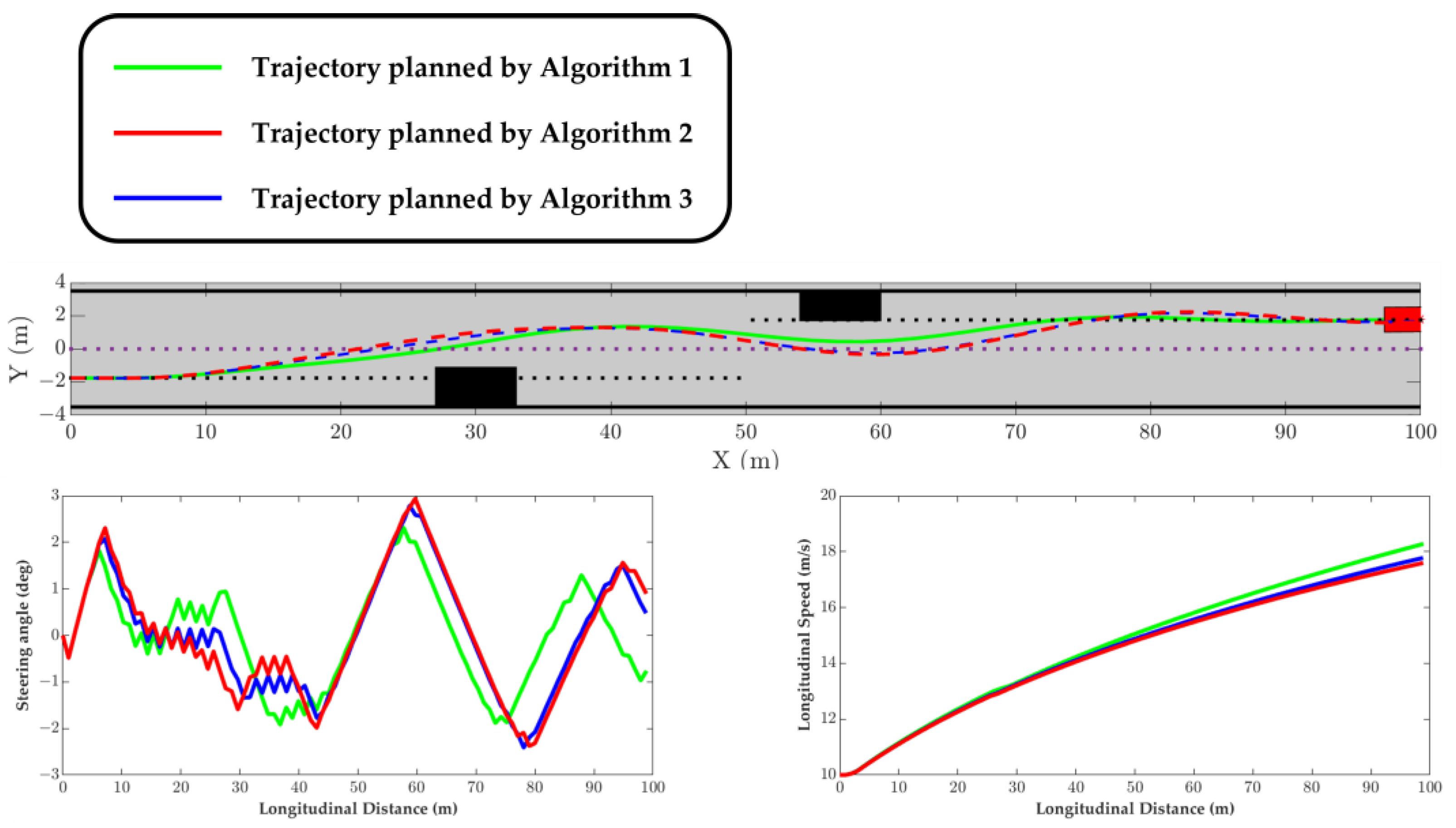
To assess the effectiveness of the proposed double-layer MPC approach, a series of experiments were conducted using MATLAB. These experiments were divided into two categories: static obstacle avoidance and dynamic obstacle avoidance. In the static scenario, the lane was occupied only by the autonomous vehicle under consideration, with stationary obstacles and no other vehicles. In the dynamic scenario, the lane contained both stationary obstacles and other vehicles. The performance of three algorithms was compared in these experiments. Algorithm 1 corresponds to the double-layer MPC algorithm proposed in this paper. Algorithm 2 represents a double-layer MPC algorithm proposed in [14], which utilizes a center point-based obstacle avoidance approach. In Algorithm 2, the upper module employs a point mass model, while the lower module employs a four-wheel nonlinear model. Algorithm 3 corresponds to a single-layer MPC algorithm proposed in the literature [13]. In Algorithm 3, the same nonlinear vehicle dynamics model used as the lower module in this paper is adopted, and similar tire load constraints are considered. However, the load constraint in Algorithm 3 is only applicable to the front two tires, while in this paper, four loads are considered. The collision avoidance constraints used in Algorithm 3 are the same as those used in Algorithm 2.

The lane setting for the autonomous vehicle involves tracking Lane 1 for the first 50 m and Lane 2 for the subsequent 50 m. The width of each lane is specified to be 3.5 m, resulting in a total lane length of 100 m. It is important to note that the reference waypoints for the lane are positioned in the center of the lane. We assume that the autonomous vehicle travels on a flat surface, the autonomous vehicle state estimations are exact, the autonomous vehicle parameters are constant, and experiments can acquire friction coefficients of the tire-terrain interaction parameters.

The simulations are performed utilizing MATLAB software, with the Nonlinear Model Predictive Control algorithm being modeled using the toolbox CASADI [22]. The nonlinear solver, IPOPT, is employed for this purpose. The model parameters used in the simulations are summarized in

Table 1. Simulation parameters.

Symbol	Value	Unit
M	2600	kg
I	3989	kg·m2
Lf, Lr	1.5, 1.7	m
W	1.5	m
ΔT	[0.05, 0.1]	s
N	30	-
μzx	800	N/(m/s2)
μzyf	679	N/(m/s2)
μzyr	1079	N/(m/s2)
[Jerk_min, Jerk_max]	[−5, 5]	m/s3
[vx_min, vx_max]	[0, 25]	m/s
[Str_min, Str_max]	[−5, 5]	deg/s
[δ_min, δ_max]	[−30, 30]	deg
F_threshold	1000	N
a_term	1270	N
b_term	90	N
Wlift_load	0.05	-
$Q_z^{HL},Q_t^{HL}$	Diag([0.01, 0.01])	-
$Q_u^{HL}$	Diag([0.05, 0.05, 0.05, 0.05, 0.005])	-
$Q_z^{LL},Q_t^{LL}$	Diag([0.025, 0.025])	-
$Q_u^{HL}$	Diag([0.015, 0.015]	-
$W_{pos}^{HL},W_t^{HL}$	0.02	-
$W_{pos}^{LL},W_t^{LL}$	0.03	-
$W_u^{HL},W_u^{LL}$	0.01	-
Pred_dist	50	m
Safety_dist	0.3	m

.

In Experiment 1, obstacles are positioned at 30 m and 55 m to obstruct the tracked lanes. The planned trajectories are depicted in Figure 4. The results of Experiment 1 demonstrate that all three algorithms successfully avoid the statics obstacles. Comparison between the algorithms reveals that Algorithm 1 has a faster lane retraction ability than Algorithms 2 and 3.

In Experiment 2, a narrow area is set up at 30 m. The safe distance is defined as 0.3 m, with a vehicle body width of 1.5 m and a narrow area width of 2.1 m. Based on these parameters, it can be theoretically deduced that any discrepancy in calculating the obstacle avoidance distance would fail in the trajectory planning process. The results of the lane tracking algorithms are visualized in Figure 5. Algorithm 1 demonstrates the ability to successfully traverse the narrow area, as it employs a non-approximation obstacle calculation scheme. Conversely, Algorithms 2 and 3 cannot plan their trajectories through the area due to their adoption of a center point-based obstacle avoidance algorithm, which results in the loss of crucial geometric information and an inability to plan trajectories in narrow environments.

Experiments conducted in static scenes demonstrate that Algorithm 1 can plan trajectories closer to the lane, owing to its non-approximation-based method for obstacle avoidance. This results in more accurate tracking of the original lane. Additionally, Algorithm 1 utilizes a double-layer structure, with the lower layer MPC tracking the replanned trajectory. This design contributes to the stability of the algorithm.

In the dynamic scenario, three moving neighboring vehicles are considered.

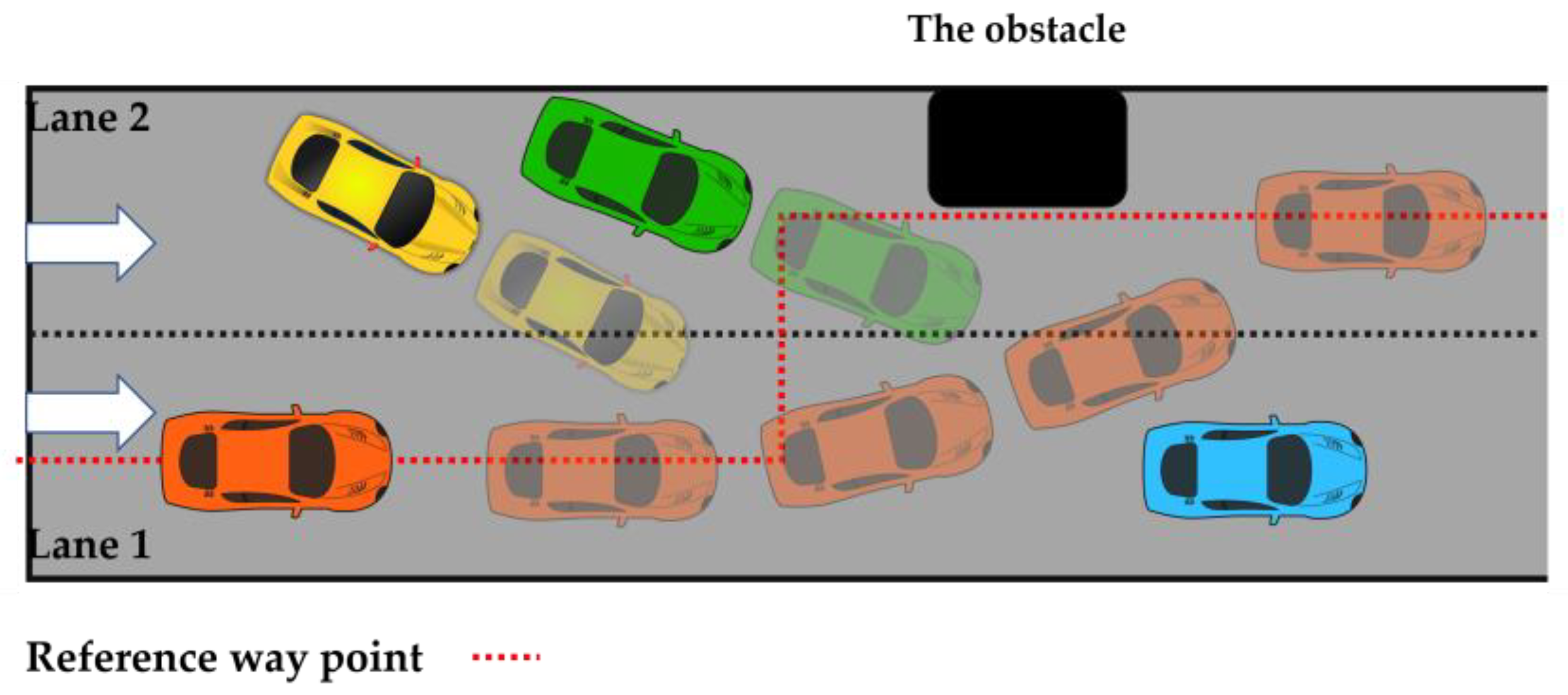
In Experiment 3, all neighboring vehicles are established with a constant velocity of 6 m/s, and the yaw angle is fixed at 0 degrees. The initial positions of the vehicles are set at 20 m, 30 m, and 40 m, as depicted in the schematic diagram presented in Figure 6. The movement of the three vehicles resulted in a narrow passing space.

The results of Experiment 3 are presented in Figure 7, and reveal that Algorithm 1 can successfully navigate the passing maneuver without difficulty. The ego vehicle can plan a more active dynamic collision avoidance path after increasing the states of the neighbor vehicle.

Conversely, Algorithm 2 can plan a trajectory, but exhibits a tire load close to 0, thus presenting a risk of rollover. Algorithm 3, however, cannot complete the overtaking maneuver, instead only being capable of tracking the lane at a low speed. In Algorithm 3, the autonomous vehicle is always at the back of the vehicle group because it cannot plan a path through the group.

In Experiment 4, a static obstacle is positioned at a distance of 50 m, with neighboring vehicles maintaining a speed of 6 m/s. Vehicle 1 and Vehicle 2 are driven in the direction of 1 and 0.5 rad towards Lane 1, while Vehicle 3 is stationed in Lane 1 in the direction of 0 rad. This setup creates a scenario in which the ego vehicle encounters obstacles during its transition from Lane 1 to Lane 2. Due to the presence of Vehicle 3 as a fixed obstacle in Lane 1, the likelihood of a three-vehicle collision is high. To prevent such a collision, the ego vehicle needs to maneuver through the cluster of vehicles as swiftly as possible. A schematic representation of the scenario is depicted in Figure 8. The results of Experiment 4, presented in Figure 9, demonstrate that Algorithm 1 can successfully plan a compact overtaking path to avoid the collision, while other algorithms failed to complete the trajectory planning.

The average time of the three algorithms is presented in

Table 2. The average computation time.

	Algorithm 1	Algorithm 2 [14]	Algorithm 3 [13]
Experiment 1	0.312 s	0.318 s	0.327 s
Experiment 2	0.321 s	0.331 s	0.332 s
Experiment 3	0.397 s	0.525 s	0.574 s
Experiment 4	0.382 s	0.441 s	0.513 s

. In the static experiment, there is only a minimal difference in time between the algorithms. Algorithm 1 does not exhibit a clear computational advantage. In experiment 3, Algorithm 3 cannot plan an overtaking trajectory, leading to a low-speed collision-free trajectory and a low average time. However, in the dynamic scenario of overtaking, Algorithm 1 performs slightly better than Algorithm 3, although its computational advantage is not substantial. On average, Algorithm 1 performed with the lowest time. These results suggest that using a double-layer structure for trajectory planning and tracking can reduce the computational burden and support the real-time deployment of the algorithm.

The stability of the MPC algorithm presents a challenging problem in the field of autonomous driving. However, the vehicle’s proximity to the predetermined lane has been theorized to impact the algorithm’s trajectory planning and tracking stability. The double-layer MPC algorithm separates the tasks of trajectory planning and trajectory tracking. This structure enables the upper layer module to plan a trajectory that is as close as possible to the predetermined lane. The lower module then tracks the replanned trajectory, resulting in a more stable algorithm than the single-layer MPC algorithm. As demonstrated in Figure 4, Figure 5, Figure 7 and Figure 9, the planned trajectories of the double-layer MPC algorithm are more closely aligned with the predetermined lanes, and theoretically, this algorithm has better stability than the algorithms proposed in [13,14].

5. Conclusions

This paper presents a novel double-layer model predictive control lane tracking approach for on-road autonomous vehicles to address safety concerns in complex traffic conditions. The results of four experiments considering static and dynamic obstacles demonstrate that the double-layer MPC lane tracking algorithm proposed in this paper outperforms the single-layer MPC [13] and double-layer MPC [14] in terms of performance, computational time, and stability. This improved performance is attributed to three factors:

(1)

The double-layer structure, which separates the trajectory planning and trajectory tracking tasks, making the motion control task more straightforward and easily solvable by MPC. In contrast to the reports in the literature [13,14], the double-layer structure proposed in this paper avoids the long trajectory planning time using a high-fidelity model in the single-layer MPC proposed in the literature [13].

(2)

The dynamic collision avoidance constraint design uses the smooth and non-approximate calculation of obstacle distances and the augmentation of the states of neighboring vehicles. Due to this calculation method’s smoothness and strong duality, introducing this collision avoidance constraint in the upper layer module does not significantly increase the computational complexity. In contrast to the tecniques in the literature [13,14], these methods can effectively ensure dynamic collision avoidance in narrow environments.

(3)

Including tire load constraints improves vehicle safety by avoiding rollover hazards. In contrast to the mtehods in the literature [13,14], the algorithm proposed in this paper provides enhanced safety features for the vehicle in complex traffic environments.

References

- Guo, J.; Kurup, U.; Shah, M. Is it Safe to Drive? An Overview of Factors, Metrics, and Datasets for Driveability Assessment in Autonomous Driving. IEEE Trans. Intell. Transp. Syst. 2020, 21, 3135–3151. [Google Scholar] [CrossRef]
- Yu, S.; Hirche, M.; Huang, Y.; Chen, H.; Allgöwer, F. Model predictive control for autonomous ground vehicles: A review. Auton. Intell. Syst. 2021, 1, 4. [Google Scholar] [CrossRef]
- Na, S.; Jang, J.; Kim, K.; Yoo, W. Dynamic vehicle model for handling performance using experimental data. Adv. Mech. Eng. 2015, 7, 168781401561812. [Google Scholar] [CrossRef] [Green Version]
- Nascimento, T.P.; Dórea, C.E.T.; Gonçalves, L.M.G. Nonholonomic mobile robots’ trajectory tracking model predictive control: A survey. Robotica 2018, 36, 676–696. [Google Scholar] [CrossRef]
- Liu, J.; Jayakumar, P.; Stein, J.L.; Ersal, T. A study on model fidelity for model predictive control-based obstacle avoidance in high-speed autonomous ground vehicles. Veh. Syst. Dyn. 2016, 54, 1629–1650. [Google Scholar] [CrossRef]
- Chen, S.; Chen, H.; Negrut, D. Implementation of MPC-Based Path Tracking for Autonomous Vehicles Considering Three Vehicle Dynamics Models with Different Fidelities. Automot. Innov. 2020, 3, 386–399. [Google Scholar] [CrossRef]
- Alrifaee, B.; Maczijewski, J.; Abel, D. Sequential Convex Programming MPC for Dynamic Vehicle Collision Avoidance. In Proceedings of the 2017 IEEE Conference on Control Technology and Applications (CCTA), Mauna Lani Resort, HI, USA, 27–30 August 2017; pp. 2202–2207. [Google Scholar]
- Alrifaee, B.; Mamaghani, M.G.; Abel, D. Centralized non-convex model predictive control for cooperative collision avoidance of networked vehicles. In Proceedings of the 2014 IEEE International Symposium on Intelligent Control (ISIC), Juan Les Pins, France, 8–10 October 2014; pp. 1583–1588. [Google Scholar]
- Franco, A.; Santos, V. Short-term Path Planning with Multiple Moving Obstacle Avoidance based on Adaptive MPC. In Proceedings of the 2019 IEEE International Conference on Autonomous Robot Systems and Competitions (ICARSC), Porto, Portugal, 24–26 April 2019; pp. 1–7. [Google Scholar]
- Laurense, V.A.; Goh, J.Y.; Gerdes, J.C. Path-tracking for autonomous vehicles at the limit of friction. In Proceedings of the 2017 American Control Conference (ACC), Seattle, WA, USA, 24–26 May 2017; pp. 5586–5591. [Google Scholar]
- Zong, C.; Miao, Q.; Zhang, B.; Yu, Z. Research on rollover warning algorithm of heavy commercial vehicle based on prediction model. In Proceedings of the 2010 International Conference on Computer, Mechatronics, Control and Electronic Engineering, Changchun, China, 24–26 August 2010; p. 5610126. [Google Scholar]
- Hang, P.; Xia, X.; Chen, G.; Chen, X. Active Safety Control of Automated Electric Vehicles at Driving Limits: A Tube-Based MPC Approach. IEEE Trans. Transp. Electrif. 2022, 8, 1338–1349. [Google Scholar] [CrossRef]
- Liu, J.; Jayakumar, P.; Stein, J.L.; Ersal, T. Combined Speed and Steering Control in High-Speed Autonomous Ground Vehicles for Obstacle Avoidance Using Model Predictive Control. IEEE Trans. Veh. Technol. 2017, 66, 8746–8763. [Google Scholar] [CrossRef]
- Gao, Y.; Lin, T.; Borrelli, F.; Tseng, E.; Hrovat, D. Predictive Control of Autonomous Ground Vehicles With Obstacle Avoidance on Slippery Roads. In Proceedings of the ASME 2010 Dynamic Systems and Control Conference, ASMEDC, Cambridge, MA, USA, 12–15 September 2010; Volume 1, pp. 265–272. [Google Scholar]
- Mayne, D.Q.; Rawlings, J.B.; Rao, C.V.; Scokaert, P.O.M. Constrained model predictive control: Stability and optimality. Automatica 2000, 36, 789–814. [Google Scholar] [CrossRef]
- Borrelli, F.; Falcone, P.; Keviczky, T.; Asgari, J.; Hrovat, D. MPC-based approach to active steering for autonomous vehicle systems. Int. J. Veh. Auton. Syst. 2005, 3, 265. [Google Scholar] [CrossRef]
- Abbas, M.A.; Milman, R.; Eklund, J.M. Obstacle avoidance in real time with Nonlinear Model Predictive Control of autonomous vehicles. In Proceedings of the 2014 IEEE 27th Canadian Conference on Electrical and Computer Engineering (CCECE), Toronto, ON, Canada, 19 May 2017; pp. 1–6. [Google Scholar]
- Lee, J.H. Model predictive control: Review of the three decades of development. Int. J. Control. Autom. Syst. 2011, 9, 415–424. [Google Scholar] [CrossRef]
- Gao, Y.; Gray, A.; Tseng, H.E.; Borrelli, F. A tube-based robust nonlinear predictive control approach to semiautonomous ground vehicles. Veh. Syst. Dyn. 2014, 52, 802–823. [Google Scholar] [CrossRef]
- Dudekula, A.B.; Naber, J.D. Algorithm Development for Avoiding Both Moving and Stationary Obstacles in an Unstructured High-Speed Autonomous Vehicular Application Using a Nonlinear Model Predictive Controller. SAE Int. J. Connect. Autom. Veh. 2020, 3, 161–191. [Google Scholar] [CrossRef]
- Zhang, X.; Liniger, A.; Borrelli, F. Optimization-Based Collision Avoidance. IEEE Trans. Control. Syst. Technol. 2021, 29, 972–983. [Google Scholar] [CrossRef] [Green Version]
- Andersson, J.A.E.; Gillis, J.; Horn, G.; Rawlings, J.B.; Diehl, M. CasADi: A software framework for nonlinear optimization and optimal control. Math. Program. Comput. 2019, 11, 1–36. [Google Scholar] [CrossRef]
Figure 1.
The process of selection of reference waypoints.
Figure 2.
Top view of bicycle model of vehicle.
Figure 3.
The schematics of the double-layer MPC-based lane tracking method.
Figure 4.
The results of Experiment 1.
Figure 5.
The results of Experiment 2.
Figure 6.
The sketch of the scenario in Experiment 3.
Figure 7.
The results of Experiment 3.
Figure 8.
The sketch of the scenario in Experiment 4.
Figure 9.
The results of Experiment 4.