Research on Fault Diagnosis of HVAC Systems Based on the ReliefF-RFECV-SVM Combined Model

Abstract

A fault diagnosis method of heating, ventilation, and air conditioning (HVAC) systems based on the ReliefF-recursive feature elimination based on cross validation-support vector machine (ReliefF-RFECV-SVM) combined model is proposed to enhance the diagnosis accuracy and efficiency. The method initially uses ReliefF to screen the original features, selecting those that account for 95% of the total weight. The recursive feature elimination based on cross validation (RFECV), based on a random forest classifier, is then applied to select the optimal feature subset according to diagnostic accuracy. Finally, a support vector machine (SVM) model is constructed for fault classification. The method is tested on seven typical faults of the ASHRAE 1043-RP water chiller dataset and three typical faults of an air-cooled self-built air conditioner simulation dataset. The results show that the ReliefF-RFECV-SVM method significantly reduces diagnosis time compared to SVM, shortening it by about 50% based on the ASHRAE 1043-RP dataset, while achieving an overall accuracy of 99.98%. Moreover, the proposed method achieves a comprehensive diagnosis accuracy of 99.97% on the self-built simulation dataset, with diagnosis time the reduced by about 65% compared to single SVM.

1. Introduction

Heating, ventilation, and air conditioning (HVAC) systems, such as chillers and air conditioning systems, are extensively used in large commercial buildings. HVAC systems consume more than 50% of the total energy in buildings [1,2], with chillers being one of the typical representatives of HVAC systems, accounting for 40% of the total HVAC energy consumption and 25% of the total HVAC maintenance costs [3,4]. When chillers malfunction, HVAC systems’ efficiency can be reduced by 15–30%, leading to increased energy consumption, poor indoor/outdoor air quality [5], and gradual loss of system functionality. Faults diagnosis in chillers can reduce energy consumption and maintenance costs by 20–50% [6]. Therefore, the fault diagnosis of HVAC systems is critical for energy conservation, cost reduction, emission reduction, and equipment efficiency improvement.

In recent years, many scholars have conducted research on the fault diagnosis of HVAC systems [7,8,9,10,11] and other related systems [12,13], which can be mainly divided into three categories: physics-based, knowledge-based, and data-driven methods. Due to their high flexibility and generalization ability, data-driven methods demonstrate better adaptability to various application scenarios and data distributions and have become a current research focus. Machine learning is one of the important tools used to achieve data-driven methods. Zhang et al. [14] proposed a novel integrated multitasking intelligent bearing fault diagnosis scheme with the aid of representation learning under imbalanced sample conditions, which realizes bearing fault detection, classification, and unknown fault identification. Zhang et al. [15] proposed a data-driven model for interactive remaining useful life (RUL) prediction of lithium-ion batteries, called PF-BiGRU-TSAM (particle filter-temporal attention mechanism-bidirectional gated recurrent unit). This method combines the advantages of data-driven approaches and model-based methods, allowing for the reflection of the importance of different time instances and the uncertainty of the degradation process. Xu et al. [16] proposed a fault diagnosis method that combines heterogeneous data normalization and domain adversarial neural networks, and established a general transfer application framework for chiller units to achieve fault diagnosis of a target chiller unit using an information-rich source chiller unit. Chen et al. [17] proposed a chiller fault detection method based on global density-weighted support vector data description to better reflect the data distribution and improve the detection accuracy. Yan et al. [18] used a one-dimensional convolutional neural network (1DCNN) to directly input raw data without the need for data preprocessing for fault diagnosis of chiller units, and achieved good diagnostic results. Chiller units often encounter data imbalance problems because it is difficult to obtain fault data for various typical faults during operation, and there are more normal operation data. To solve this problem, Shen et al. [19] proposed an enhanced data-driven fault diagnosis method based on self-attention deep learning models which generates artificial fault data using a stable synthetic minority over-sampling technique for data augmentation and achieves fault diagnosis using a self-attention mechanism-based time convolutional network to improve diagnostic accuracy.

To use machine learning for fault diagnosis of HVAC systems, it is necessary to perform feature extraction on the data, select suitable models, train and optimize the models, and finally evaluate the fault diagnosis performance of the models using a dataset. Feature selection is often the first stage in the fault diagnosis process and plays an important role. It helps to identify important features, eliminate noise and irrelevant information, and reduce the dimensionality of data. Using a reasonable feature selection method not only reduces the cost of installing sensors in engineering applications but also improves the predictive accuracy, robustness, and interpretability of the diagnostic model [20]. Therefore, it is essential to carefully select appropriate features to optimize fault diagnosis in HVAC systems. Gao et al. [21] proposed a feature selection method based on correlation analysis and experience, which analyzed the sensitive parameters of typical faults in chiller units through global sensitivity analysis based on a random forest fault diagnosis model and screened sensitive features for secondary selection through correlation analysis to form the final feature subset. Zhou et al. [22] used the light gradient boosting machine (LightBGM) model to calculate feature importance to conduct initial feature selection, and then used the recursive feature elimination method for secondary selection to form the final feature subset, and finally applied the LightBGM model for fault diagnosis of chiller units. Currently, more and more feature selection methods such as filter-based [23,24], wrapper-based [25], and embedded-based [26] techniques are being applied. Han et al. [27] used feature selection techniques based on mutual information filtering and genetic algorithms to perform feature selection in data-driven chiller unit fault detection and application, improving fault detection and diagnosis (FDD) performance while saving initial sensor costs. Yan et al. [28] proposed a cost-sensitive sequential feature selection algorithm that uses the backtrack sequential forward selection (BT-SFS) method to select the optimal sequential feature set and uses support vector machines (SVM) for fault diagnosis.

Although filter and wrapper algorithms are widely used for feature selection, single filter or wrapper algorithms have their own advantages and disadvantages. Filter-based feature selection methods have a simple structure and fast training speed, but often do not consider the correlation between features during feature selection and cannot effectively eliminate redundant features. In contrast, wrapper-based methods consider feature interactions, enabling them to effectively eliminate redundancy. However, the search process and classifier combination in wrapper-based methods can result in a high time complexity when searching for the optimal feature subset [29].

Due to the ReliefF in the filter method, it can efficiently handle high-dimensional data and demonstrate good robustness and generalization performance. However, it has certain limitations in eliminating redundant features. In wrapper methods, RFECV conducts adaptive feature selection through cross-validation, effectively eliminating redundant features and avoiding overfitting and underfitting, but it has slower training speed. Therefore, to address the limitations of single filter or wrapper feature selection algorithms, we combined the filter-based ReliefF method with the wrapper-based RFECV method. This combination aims to select a subset of features highly relevant to the fault and with the least redundancy while maintaining efficiency. Subsequently, an SVM model is applied to classify the fault. The newly proposed fault diagnosis method for HVAC systems based on ReliefF-RFECV-SVM is validated using the ASHRAE 1043-RP dataset and simulation data, demonstrating its effectiveness and feasibility.

The ReliefF-RFECV-SVM method enables efficient selection of a feature subset with high relevance to the fault and minimal redundancy, facilitating effective fault diagnosis in HVAC systems. The main contributions of this paper can be summarized as follows:

(1)

Combining the ReliefF in the filter method and the recursive feature elimination method with cross-validation in the wrapper algorithm, a feature selection method based on ReliefF-RFECV is proposed. On the basis of effectively screening redundant features considering the correlation between features, the method aims to maximize the training speed and efficiently select the feature subset with minimal redundancy and strong relevance to the fault.

(2)

The task is to develop a simulation model of an air conditioner using Amesim software, simulate typical faults and normal states of the air conditioner under various operating conditions, and generate a simulation dataset. This dataset will include data from multiple operating conditions and can be used for fault detection and diagnosis.

(3)

The approach involves using an SVM model to diagnose faults using the selected optimal feature subset. This methodology aims to improve the accuracy of fault diagnosis.

(4)

The proposed method based on ReliefF-RFECV-SVM is validated using the ASHRAE 1043-RP experimental dataset and the simulation dataset. The results show that the proposed fault diagnosis method has high diagnosis accuracy and efficiency on both the chiller unit and the air conditioning system, and strong generalization ability.

2. ReliefF-RFECV-SVM Combined Model

Using ReliefF-RFECV to select features and combining it with a data-driven SVM model for fault diagnosis of HVAC system, the methodological flow is illustrated in Figure 1.

As shown in Figure 1, the ReliefF-RFECV-SVM model consists of four parts: data preprocessing, feature selection, model construction and fault diagnosis. Firstly, the collected dataset from the HVAC system is preprocessed. Then, the ReliefF-RFECV algorithm is used for feature selection. After that, the SVM model is constructed and trained using the selected features from the training set. Finally, the trained diagnostic model is applied for fault diagnosis. The flow involves three main steps, as follows:

(1)

Operating data from the HVAC system, including normal and fault conditions, are collected and pre-processed. The pre-processing involves removing non-stationary data and rejecting outliers using the Lajda criterion. The collected data are also normalized to eliminate the impact of data dimensionality.

(2)

The Relief-RFECV feature selection algorithm is used to filter the features of the dataset after data preprocessing. Firstly, the features with weights up to 95% of the total weights are filtered using the ReliefF method to form a feature subset, then the feature subset is screened again by the RFECV method, and the subset with the highest accuracy is selected as the optimal feature subset after constructing a random forest classifier for 10 times cross-validation.

(3)

A multi-classification SVM model is initialized and constructed, with 30% of the optimal feature subset randomly selected as the training set and the remaining 70% as the test set. The training set is used to train the multi-classification SVM model, with the model parameters optimized through grid search and cross-validation. The accuracy of the final fault diagnosis model is verified using the test set.

2.1. ReliefF-RFECV Feature Selection Method

2.1.1. Introduction of the ReliefF

Relief is a method to select features by calculating the weight of features for binary classification problems. In order to solve the problem that Relief cannot perform multi-classification, Kononenko [30] proposed the ReliefF, which optimizes the weight update formula by introducing the idea of “K-Nearest Neighbors (KNN)” to the Relief to enable it to perform feature selection for multiple classification problems and regression problems. The ReliefF is a filtered feature optimization algorithm with low computational complexity which is suitable for use when performing multiple classification and regression prediction. The core idea is that excellent features can bring similar samples close and alienate heterogeneous samples. Euclidean distance is used to calculate the degree of similarity between all samples and a randomly selected sample R. The k samples with the greatest correlation are selected as the nearest neighbor samples from similar and dissimilar samples, respectively, and the inter- and intra-class distances between randomly selected sample instances and similar and dissimilar nearest neighbor samples are evaluated several times to calculate the weight of each feature. The feature weights are calculated as follows:

$$W_f^{class\left(x_i\right)}=W_f^{class(x_i-1)}+\frac{1}{n}\left\{\frac{{\sum }_{c\ne class}^{class\left(x\right)}{D}_f(x_i,M(x_i\left)\right)}{(n-1)m_{class\left(x\right)}}\right.-\left.\frac{D_f(x_i,H(x_i\left)\right)}{m_{class\left(x\right)}}\right\}$$

(1)

$$D_f(i,j)=\sqrt{\sum _f{(i_f-j_f)}^2/{\sigma }_f}$$

(2)

In Equations (1) and (2), x is the category; x_i is the samples in that category; n is the number of categories; m_class(x) is the number of samples in category x; D_f (x_i, H(x_i)) is the distance between the x_i and the nearest similar samples; D_f (x_i, M(x_i)) is the distance between x_i and the nearest heterogeneous samples; and i and j are two different samples and are the standard deviation of the feature.

The features are ranked according to the final calculated feature weights. The higher the feature weight, the stronger the classification ability of the feature, so the features with larger feature weights can be selected and the features with smaller weights can be eliminated, thus achieving feature screening.

2.1.2. Introduction of the RFECV

Recursive feature elimination based on cross validation (RFECV) is a feature selection method that combines cross-validation with the recursive feature elimination (RFE) algorithm. The RFECV consists of two stages. First, in the RFE stage, the importance of each feature is ranked, and the least important features are recursively eliminated until the desired number of features is obtained. Second, in the cross-validation stage, different numbers of features are selected based on their importance and cross-validated to determine the optimal number of features with the highest average score. Compared to the RFE, RFECV not only determines the optimal number of features but also reduces overfitting and maximizes valid information extraction from limited data.

2.1.3. Introduction and Construction of the ReliefF-RFECV

ReliefF is relatively simple to use for multi-classification feature selection, but does not take into account the correlation between features. The higher the weight of the feature calculated by ReliefF algorithm, the higher the relevance of the feature class, but it will contain redundant features. The feature subset filtered by the ReliefF method only is a feature subset formed by combining features with strong class correlation, which cannot effectively remove redundant features, thus affecting the classification effect. The RFECV uses a combination with a classifier and multiple cross-validation to select the subset of features with the best classification effect using the classification recognition rate as the evaluation index, but this method has a complex computing process and high time cost. Therefore, the ReliefF can be combined with the RFECV, fusing the advantages of both algorithms to select the best subset of features. The ReliefF-RFECV algorithm calculates the feature weights of all features using the ReliefF. Firstly, it removes irrelevant features according to the weight threshold, further screens the filtered features by the RFECV, and selects the feature subset with the best classification effect as the screening results through multiple cross-validation results. This method can obtain the best feature set of classification with the maximum correlation between features and the minimum mutual redundancy. The method steps are shown in Figure 2.

2.2. Multi-Classification Fault Diagnosis Method Based on SVM

Support vector machine (SVM) is a popular machine learning method that aims to classify data by finding the optimal plane that maximizes the interval between different types of variables in the feature space. It is widely used in data classification, regression fitting, and outlier detection. SVM has been successful in many practical diagnostic applications due to its ability to generalize and produce accurate predictions [31,32,33,34]. It is memory-efficient and can handle large datasets with ease. Initially, SVM was used for binary classification problems, but it can be extended to multi-classification problems by combining multiple binary SVM classifiers. The basic structure of an SVM classifier is shown in Figure 3.

Taking the binary classification data as an example, given training sample set Di = (x_i, y_i), i = 1…, l, where x_i inputs the samples, y_i is the labels of the two classes, and l is the number of samples, its hyperplane can be calculated using Equation (3), where b is the deviation and the weight vector. The interval of sample points to the hyperplane can be calculated using Equation (4).

$$\omega x+b=0$$

(3)

$${\delta }_i=\frac{1}{‖\omega ‖}\left|g\left(x_i\right)\right|$$

(4)

In order for the training samples to be classified correctly while ensuring the maximum interval, the two-class classification problem is transformed into a minimax problem with constraints:

$$min\frac{1}{2}{‖\omega ‖}^2$$

(5)

$$S.t. y_i\left(\omega x_i+b\right)\ge 1 i=1,\dots ,l$$

(6)

Equation (6) is used to maximize values with delimiters. If the output data are y_i = +1, then the delimiter becomes ≥1; conversely, if y_i = −1, then the delimiter becomes −1. Equations (5) and (6) are also known as quadratic programming (QP), and since their feasible domain is a convex set, they are also called convex quadratic programming. When dealing with linear indivisible problems, the relaxation variables and penalty factor C should be added to Equations (5) and (6), and the above convex quadratic programming problem becomes Equations (7) and (8).

$$min\frac{1}{2}{‖\omega ‖}^2+C\sum _{i=1}^l{\delta }_i$$

(7)

$$S.t. y_i\left(\omega x_i+b\right)\ge 1-{\delta }_{i}i=1,\dots ,l; {\delta }_i\ge 0$$

(8)

where C > 0 is a constant whose magnitude determines the degree of penalty for misclassified samples.

To solve the above constrained optimization problem, the Lagrange function is introduced to represent the generalized problem of finding the optimal hyperplane by applying Lagrange multipliers in pairwise form, as shown in Equations (9) and (10)

$$max W\left(a\right)=\sum _{i=1}^l{a}_i-\frac{1}{2}\sum _{i,j}^l{a}_i{a}_j{y}_i{y}_j{\phi \left(x_i\right)}^T\phi \left(x_j\right)$$

(9)

$$S.t. {\sum }_{i=1}^l{a}_i{y}_i=0,0\le a_i\le C,i=1,2,\dots ,l$$

(10)

where W(a) is the dual function, a_i and a_j are Lagrange multipliers, and the dot product can be replaced by the kernel K(x_i, x_j) according to Mercer’s theorem, as shown in Equation (11)

$$K\left(x_i,x_j\right)=\phi \left(x_i\right)·\phi \left(x_j\right)$$

(11)

The KKT condition is used to find the threshold value $b*$, so as to obtain the optimal classification decision function, as shown in Equation (12)

$$f(x)=\mathrm{s}\mathrm{g}\mathrm{n}\left(\sum _{i=1}^l{a}_i\times y_{i}K\left(x_i,x_j\right)+b*\right)$$

(12)

Optimal grid search involves testing various combinations and validating each combination to select the best model and hyperparameters. The aim is to determine the combination that results in the best model performance, which can then be chosen as the predictive model. In this study, we utilized grid search in conjunction with cross-validation to search for the optimal C-value, kernel function, and gamma value for the SVM model. Based on the classification accuracy obtained from 10-fold cross-validation, we selected the combination with the highest accuracy as the optimal parameter for the model.

3. Design of Fault Diagnosis

3.1. Data Description

Our proposed fault diagnosis method was evaluated using two datasets. Dataset 1 was obtained from the ASHRAE 1043-RP [35], which involved an experimental study of a 90-cold ton centrifugal chiller. The dataset consists of test data for 64 parameters collected under normal conditions and seven typical faults at four deterioration levels (as shown in

Table 1. Fault types and fault deterioration levels of the ASHRAE 1043-RP dataset.

Num.	Fault Type	SL1	SL2	SL3	SL4
1	Flow water of condenser Insufficient (FWC)	−10%	−20%	−30%	−40%
2	Flow water of evaporator Insufficient (FWE)	−10%	−20%	−30%	−40%
3	Refrigerant leak (RL)	−10%	−20%	−30%	−40%
4	Refrigerant over (RO)	+10%	+20%	+30%	+40%
5	Condenser fouling (CF)	−12%	−20%	−30%	−45%
6	Excessive over (EO)	+14%	+32%	+50%	+68%
7	Non-condensable gas contained (NC)	+1%	+2%	+3%	+5%

). The dataset includes 48 directly measured data and 16 indirectly calculated data. Each experiment lasted for 51,910 s, with data collected at 10 s intervals (for more details about the ASHRAE 1043-RP dataset, please refer to reference [35]).

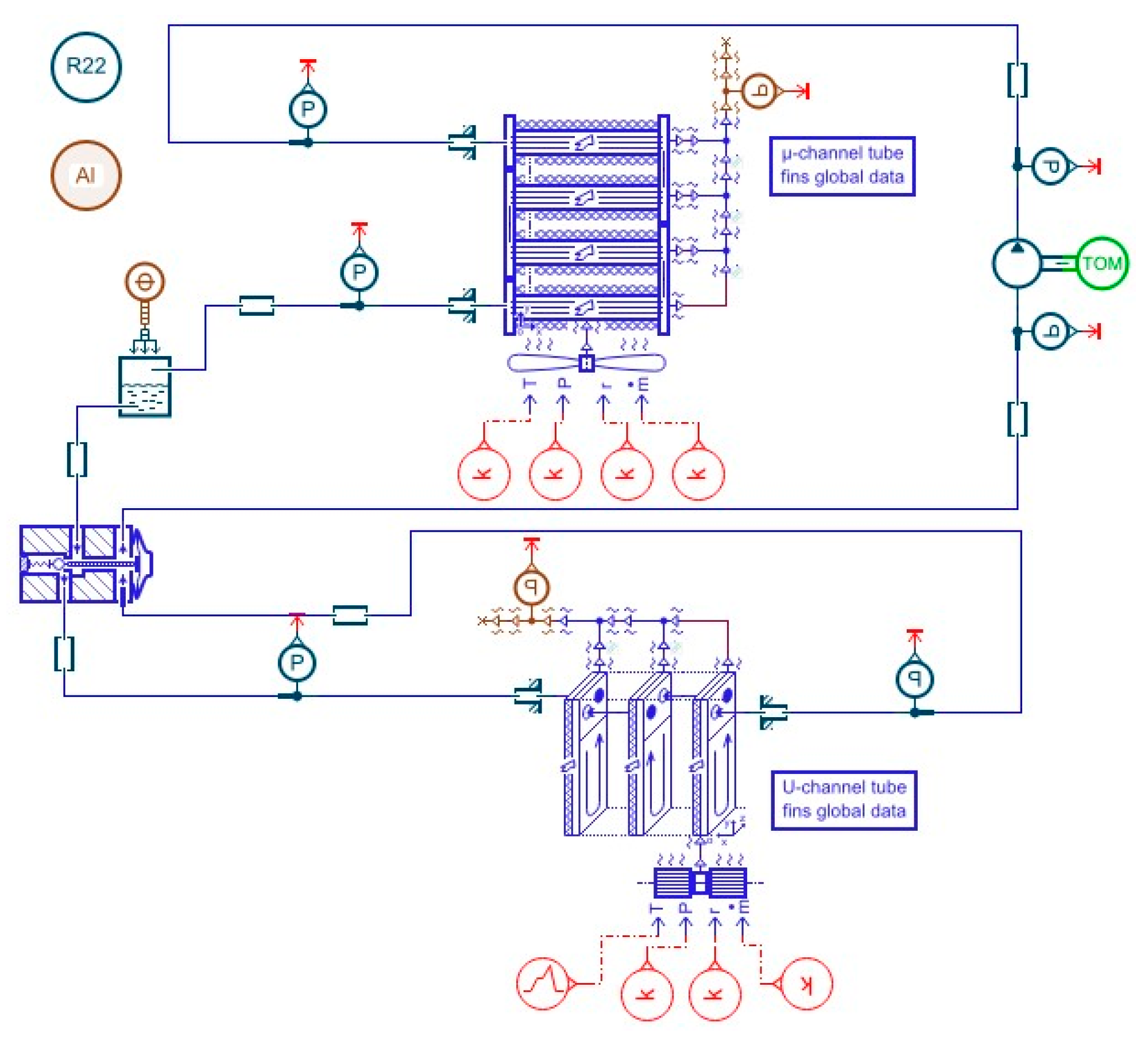
Dataset 2 is a simulation dataset created using Amesim software. A simulation model of an air conditioning system was built based on actual product parameters from a company, as depicted in Figure 4. The simulation model was used to simulate condenser fouling, compressor wear, and evaporator fouling at various working conditions ranging from 35 °C to 41 °C, with the vehicle interior temperature as the control variable. Each fault was simulated at four fault levels, as outlined in

Table 2. Fault types and fault deterioration levels of the Amesim simulation dataset.

Num.	Fault Type	Fault Introduction Method	SL1	SL2	SL3	SL4
1	Condenser Fouling (CF)	Adjust the air mass flow through the condenser	−10%	−20%	−30%	−40%
2	Compressor Wear (CW)	Change the speed of the compressor	−10%	−20%	−30%	−40%
3	Evaporator Scaling (ES)	Adjust the air mass flow through the evaporator	−10%	−20%	−30%	−40%

. The simulation was run for 7000 s under various working conditions for each fault and fault level, and 24 parameters were collected and recorded, as shown in

Table 3. Twenty-four features of the Amesim simulation dataset.

Num.	Name	Features	Num.	Name	Features
1	Lto	Exhaust temperature of condenser	13	Zto	Evaporator exhaust temperature
2	Lpo	Exhaust pressure of condenser	14	Zpo	Evaporator exhaust pressure
3	Lti	Condenser suction temperature	15	Zti	Evaporator suction temperature
4	Lpi	Condenser suction pressure	16	Zpi	Evaporator suction pressure
5	LWc	Condenser outlet humidity	17	ZWc	Evaporator outlet humidity
6	LTc	Condenser outlet temperature	18	ZTc	Evaporator outlet temperature
7	TRC	Refrigerant temperature in condenser	19	TRE	Refrigerant temperature in evaporator
8	PRC	Refrigerant pressure in condenser	20	PRE	Refrigerant pressure in evaporator
9	Yto	Exhaust temperature of compressor	21	FPc	Expansion valve outlet pressure
10	Ypo	Compressor delivery pressure	22	Fpi	Expansion valve inlet pressure
11	Yti	Compressor suction temperature	23	Qc	Specific refrigerating effect
12	Ypi	Compressor suction pressure	24	SH	Degree of superheat

.

3.2. Data Preprocessing

HVAC system operation data can be affected by various factors during collection, transportation, and storage, which can result in missing data and sudden changes, negatively impacting the fault diagnosis accuracy. Therefore, data preprocessing is required to improve the data quality. For example, in the ASHRAE 1043-RP dataset, preprocessing involves removing irrelevant features, applying steady-state filtering, using the Ljida criteria to eliminate outliers, and standardizing the data.

3.3. Feature Selection Based on the ReliefF-RFECV

Using the ASHRAE 1043-RP dataset as an example, we preprocessed the 54 features (as shown in

Table 4. Fifty-four features of the ASHRAE 1043-RP dataset.

Num.	Features	Description
1	TWI	Temperature of City Water In
2	FWE	Flow Rate of Evaporator Water
3	PO_feed	Pressure of Oil Feed
4	PO_net	Oil Feed minus Oil Vent Pressure
5	FWC	Flow Rate of Condenser Water
6	VC	Condenser Valve Position
7	TCA	Condenser Approach Temperature
8	TRC_sub	Liquid-line Refrigerant Subcooling from Condenser
9	TO_sump	Temperature of Oil in Sump
10	TO_feed	Temperature of Oil Feed
11	TR_dis	Refrigerant Discharge Temperature
12	THI	Temperature of Hot Water In
13	THO	Temperature of Hot Water Out
14	TRE	Saturated Refrigerant Temperature in Evaporator
15	PRE	Pressure of Refrigerant in Evaporator
16	T_suc	Refrigerant Suction Temperature
17	TWO	Temperature of City Water Out
18	TWED	Evaporator Water Temperature Delta
19	TEO	Temperature of Evaporator Water Out
20	Evap Tons	Calculated Evaporator Cooling Rate
21	TCO	Temperature of Condenser Water Out
22	TSI	Temperature of Shared HX Water In (in Condenser Water Loop)
23	TCI	Temperature of Condenser Water In
24	TSO	Temperature of Shared HX Water Out (in Condenser Water Loop)
25	TEI	Temperature of Evaporator Water In
26	TWEI	Temperature of Evaporator Water In
27	TWEO	Temperature of Evaporator Water Out
28	TWCI	Temperature of Condenser Water In
29	TWCO	Temperature of Condenser Water Out
30	TBI	Temperature of Building Water In (in Evaporator Water Loop)
31	TBO	Temperature of Building Water Out (in Evaporator Water Loop)
32	Cond Tons	Calculated Condenser Heat Rejection Rate
33	Cooling Tons	Calculated City Water Cooling Rate
34	Shared Cond Tons	Calculated Shared HX Heat Transfer (only valid with no water bypass)
35	Cond Energy Balance	Calculated 1st Law Energy Balance for Condenser Water Loop (only valid with no water bypass)
36	Shared Evap Tons	Calculated Shared HX Heat Transfer (should equal Shared Cond Tons with no water bypass)
37	Building Tons	Calculated Steam Heating Load
38	kW	Watt Transducer Measuring Instantaneous Compressor Power
39	COP	Calculated Coefficient of Performance
40	TEA	Evaporator Approach Temperature
41	TRC	Saturated Refrigerant Temperature in Condenser
42	PRC	Pressure of Refrigerant in Condenser
43	Tsh_suc	Refrigerant Suction Superheat Temperature
44	Tsh_dis	Refrigerant Discharge Superheat Temperature
45	P_lift	Pressure Lift Across Compressor
46	Amps	Current Draw Across One Leg of Motor Input
47	RLA%	Percent of Maximum Rated Load Amps
48	Tolerance%	Calculated Heat Balance Tolerance According to ARI 550
49	TWCD	Condenser Water Temperature Delta
50	VSS	Small Steam Valve Position
51	VM	3-way Mixing Valve Position
52	VW	City Water Valve Position
53	FWW	Calculated City Water Flow Rate
54	FWB	Calculated Condenser Water Bypass Flow Rate

, while the specific meanings of all features in the table can be found in reference [35]) by conducting ReliefF feature screening. The weights of each feature were calculated and ranked, and features with a total weight that accounts for 95% of the total weight were retained as the feature subset by weight ranking. This resulted in a subset of 46 dimensions, which are the features numbered 1 to 46 in Table 4. The subset of features obtained through ReliefF screening was further screened using the RFECV algorithm. After conducting 10-fold cross-validation using the random forest classifier, the feature subset with the highest accuracy was selected as the optimal feature subset. This subset consists of 24 features, specifically features 1 to 24 shown in Table 4.

The Amesim simulation dataset underwent feature filtering using the ReliefF-RFECV method, resulting in a 6-dimensional optimal feature subset, as listed in

Table 5. Optimal feature subset selected by means of the ReliefF-RFE method on the Amesim dataset.

Number	Name	Feature
1	Lti	Condenser suction temperature
2	Yto	exhaust temperature of compressor
3	LWc	Condenser outlet humidity
4	ZWc	Evaporator outlet humidity
5	Qc	specific refrigerating effect
6	SH	degree of superheat

.

3.4. Evaluation Metrics for Classification Performance

The fault diagnosis model proposed in this paper is essentially a multi-classification problem. The trained model effectively distinguishes normal operation and seven types of faults. Commonly used performance evaluation indexes for multi-classification include accuracy (AC), recall (R), precision (P), and F₁ [36,37]. P is used to evaluate the accuracy of the model for a certain type of fault diagnosis, while R is used to evaluate the detection ability of a certain type of fault. P and R, respectively, evaluate the recognition ability of multi-classification models for a certain type of samples, which often constrain each other. F₁ integrates P and R to better evaluate the classification effect, and each evaluation index is shown in Equations (13)–(16). In multi-classification fault diagnosis, a confusion matrix is commonly used to evaluate the diagnostic results more intuitively and comprehensively. The results on the diagonal represent the number of correctly predicted samples, while the remaining positions represent the number of incorrectly predicted samples. True positives (TP), true negatives (TN), false positives (FP) and false negatives (FN) can be obtained directly through the confusion matrix, as shown in

Table 6. Description of confusion matrix.

	True Label
Predict label		0	1
	0	TP	FP
	1	FN	TN

.

$$Accuracy=\frac{TP+TN}{TP+TN+FP+FN}$$

(13)

$$Recall=\frac{TP}{TP-FN}$$

(14)

$$Precision=\frac{TP}{TP-FP}$$

(15)

$$F_1=\frac{2\times Recall\times Precision}{(Recall+Precision)}$$

(16)

4. Analysis of Fault Diagnosis Results

4.1. Diagnostic Results on ASHRAE 1043-RP Dataset

After preprocessing the public dataset, two datasets were created: original dataset 1 and ReliefF-RFECV dataset 1, consisting of 54 and 24 parameters (as shown in Table 4), respectively. Each dataset contained 3000 randomly selected data points for each state, totaling 24,000 data points. Overall, 30% of the data were randomly selected as the training set and the remaining 70% were used as the test set. The SVM model was used for fault diagnosis of seven typical chiller faults, and the fault diagnosis confusion matrix for fault level 1 is shown in Figure 5. The results indicate that after feature selection, the diagnostic error rates for RL and EO were significantly reduced, with only four errors remaining for the RO fault in ReliefF-RFECV dataset 1. There were no incorrect diagnoses for the other six fault types or under normal conditions.

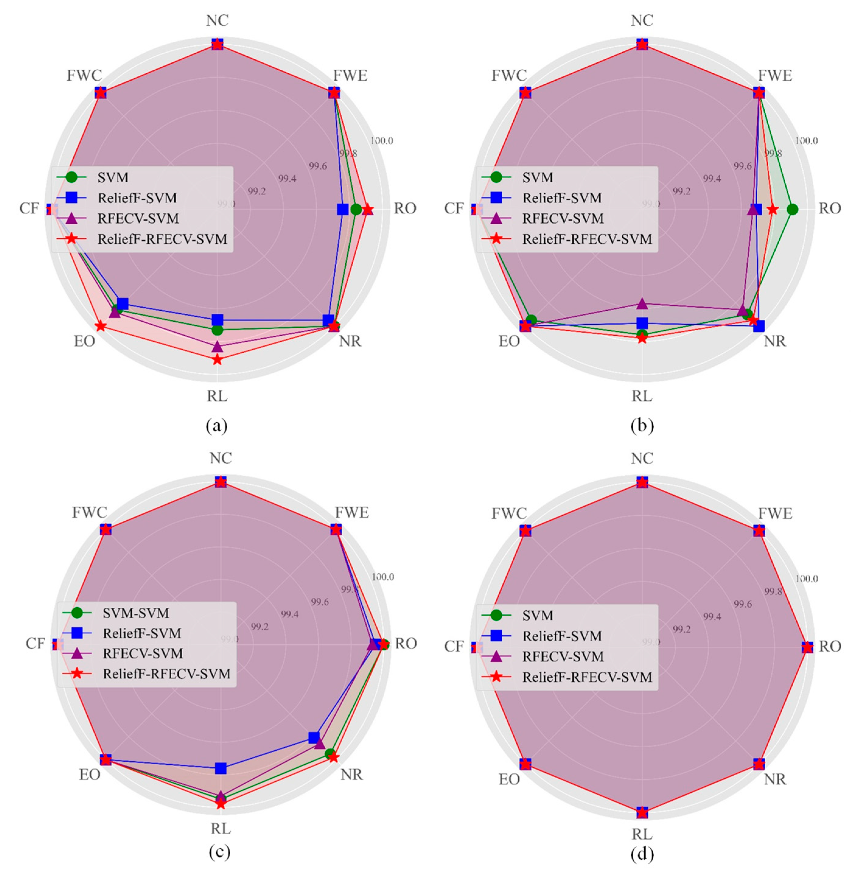
To demonstrate the effectiveness of the ReliefF-RFECV feature selection algorithm, four feature sets were constructed as control groups based on the ASHRAE 1043-RP datasets, namely the original, ReliefF, RFECV, and ReliefF-RFECV datasets. The ReliefF dataset included features with a weight sum of 95%, while the RFECV dataset was screened using the RFECV. SVM with a grid search method was used to optimize the four control datasets, and the results are presented in Figure 6 and

Table 7. Comparison of fault diagnosis results on the ASHRAE 1043-RP dataset with different feature selection algorithms (%/s).

Fault Diagnosis Method	Level 1			Level 2			Level 3			Level 4
	AC	F1	Time	AC	F1	Time	AC	F1	Time	AC	F1	Time
SVM	99.93	99.93	1256.08	99.94	99.94	1166.40	99.99	99.99	1087.98	100	100	1027.04
SVM-ReliefF	99.90	99.90	1094.64	99.92	99.92	1006.09	99.94	99.94	947.71	99.98	99.98	872.39
SVM-RFECV	99.95	99.95	557.62	99.89	99.89	512.55	99.99	99.97	479.27	100	100	445.08
SVM-ReliefF-RFECV	99.98	99.98	602.14	99.94	99.94	552.72	99.99	99.99	517.74	100	100	476.82

. It was found that the SVM-ReliefF-RFECV diagnostic method had the best diagnostic performance at levels 1–4 in the ASHRAE 1043-RP dataset. Furthermore, according to Table 7, it can be observed that compared to SVM and SVM-ReliefF, the diagnostic time of the SVM-ReliefF-RFECV method is significantly reduced, with a reduction of approximately 40% to 50%. Specifically, at fault level 1, the diagnostic time of SVM-ReliefF-RFECV decreased from 1256.08 s to 602.14 s compared to SVM, and from 1094 s to 602 s compared to SVM-ReliefF, only slightly longer than SVM-RFECV. Overall, the ReliefF-RFECV feature selection method outperforms the individual methods, ensuring high diagnostic accuracy while greatly reducing the diagnostic time and improving efficiency, and even surpassing the diagnostic accuracy of other methods.

Besides using the SVM model, the random forest and KNN classifiers were also employed for fault diagnosis. The grid search and cross-validation techniques were applied to select the optimal parameters, and the specific diagnostic results of different classifiers are shown in Figure 7 and

Table 8. Fault diagnosis results of the ASHRAE 1043-RP original dataset and ReliefF-RFECV dataset under different methods (%/s).

Fault Diagnosis Method	Level 1			Level 2			Level 3			Level 4
	AC	F1	Time	AC	F1	Time	AC	F1	Time	AC	F1	Time
SVM	99.93	99.93	1256.08	99.94	99.94	1166.40	99.99	99.99	1087.98	100	100	1027.04
SVM-ReliefF-RFECV	99.98	99.98	602.14	99.94	99.94	552.72	99.99	99.99	517.74	100	100	476.82
RF	99.80	99.80	536.95	99.83	99.83	533.20	99.95	99.95	512.28	99.99	99.99	495.89
RF-ReliefF-RFECV	99.92	99.92	388.81	99.83	99.83	378.87	99.97	99.97	370.70	99.99	99.99	354.31
KNN	98.71	98.72	29.07	98.96	98.96	25.65	99.51	99.50	24.55	99.76	99.76	24.36
KNN-ReliefF-RFECV	99.60	99.60	13.38	99.70	99.70	11.79	99.83	99.84	13.61	99.98	99.98	10.55

. Among them, the SVM-ReliefF-RFECV combined model achieved the highest diagnostic accuracy and F₁ score at levels 1–4. Although the diagnostic accuracy of the SVM model was comparable to that of the SVM-ReliefF-RFECV model at levels 2 and 4, the diagnostic time was significantly longer. Furthermore, Table 8 shows that the ReliefF-RFECV algorithm effectively improves fault diagnosis efficiency. Taking level 1 as an example, the diagnostic time of RF-ReliefF-RFECV decreased from 536.95 s to 388.81 s compared to RF, and KNN-ReliefF-RFECV reduced the diagnostic time from 29.07 s to 13.38 s compared to KNN. Both RF-ReliefF-RFECV and KNN-ReliefF-RFECV showed improved fault diagnosis accuracy compared to RF and KNN, respectively. These results confirm the feasibility of the ReliefF-RFECV feature selection algorithm and the superiority of the SVM-ReliefF-RFECV method.

4.2. Diagnosis Results of Simulation Dataset

After preprocessing, the original Amesim simulation dataset in Table 3 was used as dataset 2. After applying the ReliefF-RFECV feature selection algorithm, the ReliefF-RFECV dataset 2 was obtained, as shown in Table 5. Both datasets contain 48,000 data points, and the test and training sets were randomly divided at a 3:7 ratio. After preprocessing, both datasets were diagnosed using the SVM classifier, and the fault diagnosis confusion matrix at fault level 1 is shown in Figure 8. On the self-built simulation dataset of air conditioners, the SVM-ReliefF-RFECV diagnostic method achieved higher diagnostic accuracy. The number of cases of wrong diagnosis in refrigerant leakage was reduced from 17 to 9, the number of wrong diagnoses in compressor wear was reduced from six to five, and the number of errors in normal diagnosis was reduced from seven to five, indicating a significant improvement in diagnostic effectiveness.

Similarly, on the self-built simulation dataset of multiple working conditions, four feature datasets were constructed as control groups for fault diagnosis. The diagnostic results are shown in Figure 9 and

Table 9. Comparison of diagnosis results for the Amesim dataset with different feature selection algorithms (%/s).

Fault Diagnosis Method	Level 1			Level 2			Level 3			Level 4
	AC	F1	Time	AC	F1	Time	AC	F1	Time	AC	F1	Time
SVM	99.94	99.94	1346.83	99.96	99.95	1234.07	99.95	99.95	1163.28	99.93	99.94	1127.35
SVM-ReliefF	99.97	99.97	1112.47	99.97	99.97	1035.18	99.95	99.93	964.28	99.96	99.96	896.71
SVM-RFECV	99.97	99.97	1209.91	99.98	99.98	1105.44	99.97	99.97	1058.14	99.95	99.95	998.14
SVM-ReliefF-RFECV	99.96	99.96	483.29	99.96	99.96	410.04	99.96	99.96	372.12	99.93	99.93	353.36

. The fault diagnosis accuracy after feature screening by the ReliefF-RFECV method is slightly lower than that obtained by other feature screening methods. However, compared to the highest difference in accuracy and F₁, the decrease is only 0.03%, which still maintains a high diagnostic accuracy. Additionally, it significantly improves diagnostic time, with ReliefF-RFECV-SVM reducing the diagnostic time by over 60% compared to other methods. At level 1, ReliefF-RFECV-SVM reduced the diagnostic time by 863.54 s, 629.18 s, and 726.62 s compared to SVM, ReliefF-SVM, and RFECV-SVM, respectively. Overall, the ReliefF-RFECV feature selection method is more effective than a single method, ensuring high diagnostic accuracy while significantly reducing diagnostic time and improving efficiency.

The KNN and RF models were also utilized for fault diagnosis. The results are presented in Figure 10 and

Table 10. Fault diagnosis results of the Amesim raw dataset and ReliefF-RFECV dataset under different methods (%/s).

Fault Diagnosis Method	Level1			Level2			Level3			Level4
	AC	F1	Time	AC	F1	Time	AC	F1	Time	AC	F1	Time
SVM	99.94	99.94	1346.83	99.96	99.95	1234.07	99.95	99.95	1163.28	99.93	99.94	1127.35
SVM-ReliefF-RFECV	99.96	99.96	483.29	99.96	99.96	410.04	99.96	99.96	372.12	99.93	99.93	353.36
RF	99.81	99.92	627.01	99.90	99.91	554.48	99.92	99.92	581.07	99.88	99.89	593.86
RF-ReliefF-RFECV	99.92	99.93	452.85	99.92	99.92	432.69	99.92	99.92	433.29	99.91	99.91	400.17
KNN	99.81	99.81	14.90	99.88	99.88	15.72	99.90	99.91	15.61	99.87	99.87	15.97
KNN-ReliefF-RFECV	99.82	99.82	9.49	99.84	99.85	9.49	99.88	99.88	9.37	99.88	99.88	9.80

. As shown in Table 10, the accuracy and F₁ are the highest for fault levels 1~4. Meanwhile, for levels 2~4, the diagnostic performance of the SVM model is comparable to the best, but the diagnostic time is significantly shorter. Specifically, at fault level 2, the diagnostic time was reduced from 1234.07 s to 410.04 s. Combining the ReliefF-RFECV method with random forest and KNN classifiers improved the efficiency of each diagnostic model, further demonstrating the generalizability and feasibility of the feature selection algorithm. The SVM-ReliefF-RFECV method significantly reduces fault diagnosis time, which is essential for timely repairs and cost savings in engineering applications.

4.3. Analysis of Comparative Results

To further validate the effectiveness of the method, the Relief-RFECV feature set was compared with feature sets proposed by Ke Yan et al. [28], Y. Gao et al. [21], Guannan Li et al., and Yang Zhao et al. [38,39] on the ASHRAE 1043-RP dataset. The results are shown in Figure 11. As depicted in Figure 11, the Relief-RFECV feature subset achieves higher accuracy than other feature sets in the 1DCNN-BIGRU, KNN, RF, and SVM fault models, thus confirming the superiority of the feature selection algorithm.

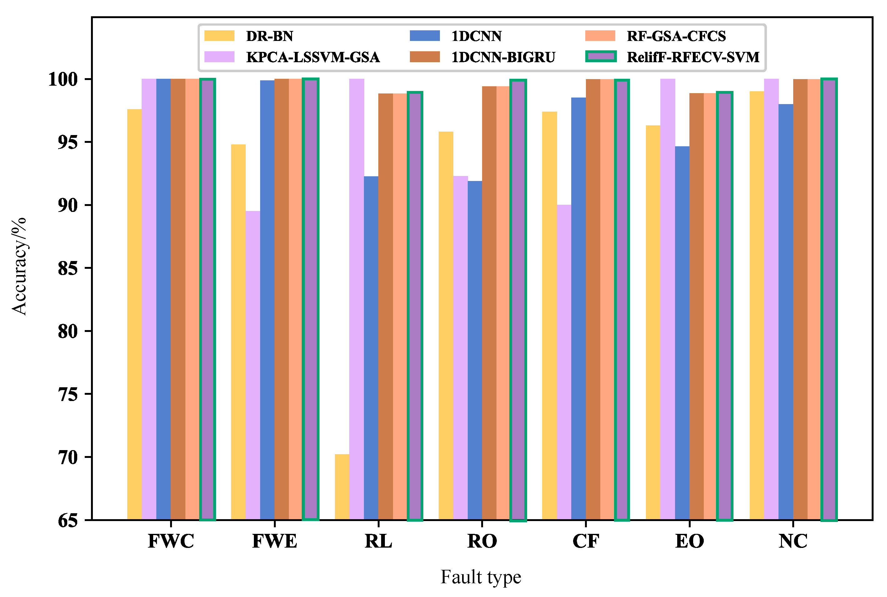
In addition, the Relief-RFECV-SVM method was compared with other proposed fault diagnosis methods (Bayesian network merged distance rejection (DR-BN) [40], kernel principle component analysis-least squares support vector machine-gravitational search algorithm (KPCA-LSSVM-GSA) [41], random forest-global sensitivity analysis-cascade feature cleaning and supplement (RF-GSA-CFCS) [21], one-dimensional convolutional neural network-bidirectional gated recurrent unit (1DCNN-BIGRU) [42] and 1DCNN [18]). As shown in Figure 12 and

Table 11. Fault diagnosis results compared with other advanced studies on the ASHRAE 1043-RP dataset (%).

Fault Diagnosis Method	The Diagnostic Accuracy of Each Fault							Overall Accuracy
	FWC	FWE	RL	RO	CF	EO	NC
DR-BN	97.6	94.8	70.2	95.8	97.4	96.3	99	93.01
KPCA-LSSVM-GSA	100.0	89.5	100.0	92.3	90	100.0	100.0	95.97
1DCNN	100.0	99.88	92.25	91.88	98.5	94.63	98.00	96.45
1DCNN-BIGRU	100.0	100.0	98.69	99.06	99.98	98.77	99.98	99.50
RF-GSA-CFCS	100.0	100.0	99.01	100.0	100.0	99.0	100.0	99.71
ReliefF-RFECV-SVM	100.0	100.0	99.94	99.93	100.0	99.98	100.0	99.98

, the proposed method achieved higher fault diagnosis accuracy for six typical faults of chiller faults. Specifically, compared to RF-GSA-CFCS, the proposed method only has a 0.06% decrease in diagnosis accuracy for the RO fault, and compared to KPCA-LSSVM-GSA, it has a 0.06% decrease in diagnosis accuracy for the RL fault and a 0.02% decrease for the EO fault. However, the proposed method demonstrated higher diagnosis accuracy for other faults, with an overall diagnosis accuracy of up to 99.98%, which is significantly better than the other methods. In conclusion, the ReliefF-RFECV-SVM diagnosis model exhibited higher accuracy compared to the aforementioned studies.

By comparing the above fault diagnosis results, it can be seen that:

(1)

This method utilizes the RelifF-RFECV algorithm for feature selection and the SVM classifier for fault diagnosis, achieving fault diagnosis for typical faults in HVAC systems on both the ASHRAE 1043-RP dataset and the self-built Amesim simulation dataset.

(2)

On the ASHRAE 1043-RP dataset, the diagnostic accuracy at level 1 is enhanced from 99.94% to 99.98% compared to the original dataset. Similarly, on the simulation dataset, the diagnostic accuracy at level 1 is improved from 99.93% to 99.96% compared to the original dataset. This method outperforms other research methods in terms of diagnostic accuracy for all faults except for RO and EO faults, which have a slightly lower accuracy rate of 0.06% and 0.02%, respectively, compared to other methods. The overall accuracy rate of this method is as high as 99.98%.

(3)

The proposed RelifF-RFECV-SVM method reduces the diagnosis time by approximately 50% compared to the SVM method, while ensuring diagnostic accuracy. Similarly, in the fault diagnosis of self-built simulation data in Amesim, the time is reduced by about 60% to 70%.

(4)

This method exhibits strong generalization, achieving accurate fault diagnosis not only on the ASHRAE 1043-RP dataset but also on the self-built simulation dataset using Amesim.

5. Conclusions

Our proposed fault diagnosis method is based on the ReliefF-RFECV-SVM combined model. Firstly, the ReliefF-RFECV method is used for feature screening to obtain the optimal subset of features closely related to faults with less redundancy. Then, the SVM classifier is combined to build a fault diagnosis model, which is trained and optimized using grid search and cross-validation to provide accurate fault diagnosis for chiller and air conditioning simulation models. This method ensures high accuracy while effectively shortening the time of fault diagnosis, thus improving the efficiency of fault diagnosis. The accuracy is 99.96% and 99.97% when the chiller fault and air conditioning simulation system fault are at level 1, respectively, indicating that this method can accurately diagnose minor faults in HVAC systems and has good generalization. However, in practical applications, sensor cost and usage frequency should also be considered when guiding the installation of important feature sensors to detect HVAC systems. Therefore, the feature selection algorithm needs further optimization based on existing information.

References

- Verhelst, J.; Van Ham, G.; Saelens, D.; Li, H. Model selection for continuous commissioning of HVAC-systems in office buildings: A review. Renew. Sustain. Energy Rev. 2017, 76, 673–686. [Google Scholar] [CrossRef]
- Beiter, P.; Elchinger, M.; Tian, T. Renewable Energy Data Book; National Renewable Energy Lab. (NREL): Golden, CO, USA, 2017. [Google Scholar]
- Yu, X.; Yan, D.; Sun, K.; Hong, T.; Zhu, D. Comparative study of the cooling energy performance of variable refrigerant flow systems and variable air volume systems in office buildings. Appl. Energy 2016, 183, 725–736. [Google Scholar] [CrossRef] [Green Version]
- Fan, Y.; Cui, X.; Han, H.; Lu, H. Chiller fault diagnosis with field sensors using the technology of imbalanced data. Appl. Therm. Eng. 2019, 159, 113933. [Google Scholar] [CrossRef]
- Yao, W.; Li, D.; Gao, L. Fault detection and diagnosis using tree-based ensemble learning methods and multivariate control charts for centrifugal chillers. J. Build. Eng. 2022, 51, 104243. [Google Scholar] [CrossRef]
- Tian, C.; Wang, Y.; Ma, X.; Chen, Z.; Xue, H. Chiller Fault Diagnosis Based on Automatic Machine Learning. Front. Energy Res. 2021, 9, 753732. [Google Scholar] [CrossRef]
- Han, S.; Shao, H.; Huo, Z.; Yang, X.; Cheng, J. End-to-end chiller fault diagnosis using fused attention mechanism and dynamic cross-entropy under imbalanced datasets. Build. Environ. 2022, 212, 108821. [Google Scholar] [CrossRef]
- Bai, X.; Zhang, M.; Jin, Z.; You, Y.; Liang, C. Fault detection and diagnosis for chiller based on feature-recognition model and kernel discriminant analysis. Sustain. Cities Soc. 2022, 79, 103708. [Google Scholar] [CrossRef]
- Gao, L.; Li, D.; Liu, X.; Liu, G. Enhanced chiller faults detection and isolation method based on independent component analysis and k-nearest neighbors classifier. Build. Environ. 2022, 216, 109010. [Google Scholar] [CrossRef]
- Huang, T.; Liang, C.; Bai, X.; Feng, Z.; Wang, F. Study on the feature-recognition-based modeling approach of chillers. Int. J. Refrig. 2019, 100, 326–334. [Google Scholar] [CrossRef]
- Yan, K.; Su, J.; Huang, J.; Mo, Y. Chiller fault diagnosis based on VAE-enabled generative adversarial networks. IEEE Trans. Autom. Sci. Eng. 2020, 19, 387–395. [Google Scholar] [CrossRef]
- Xiang, C.; Zhou, J.; Han, B.; Li, W.; Zhao, H. Fault Diagnosis of Rolling Bearing Based on a Priority Elimination Method. Sensors 2023, 23, 2320. [Google Scholar] [CrossRef]
- Wang, Z.; Luo, W.; Xu, S.; Yan, Y.; Huang, L.; Wang, J.; Hao, W.; Yang, Z. Electric Vehicle Lithium-Ion Battery Fault Diagnosis Based on Multi-Method Fusion of Big Data. Sustainability 2023, 15, 1120. [Google Scholar] [CrossRef]
- Jiusi, Z.; Ke, Z.; Yiyao, A.; Hao, L.; Shen, Y. An Integrated Multitasking Intelligent Bearing Fault Diagnosis Scheme Based on Representation Learning Under Imbalanced Sample Condition. IEEE Trans. Ind. Inform. 2023, 1, 1–12. [Google Scholar] [CrossRef]
- Jiusi, Z.; Congsheng, H.; Moyuen, C.; Xiang, L.; Jilun, T.; Hao, L.; Shen, Y.A. Data-model Interactive Remaining Useful Life Prediction Approach of Lithium-ion Batteries Based on PF-BiGRU-TSAM. IEEE Trans. Ind. Inform. 2023, 4, 1–12. [Google Scholar] [CrossRef]
- Zhu, X.; Chen, K.; Anduv, B.; Jin, X.; Du, Z. Transfer learning based methodology for migration and application of fault detection and diagnosis between building chillers for improving energy efficiency. Build. Environ. 2021, 200, 107957. [Google Scholar] [CrossRef]
- Chen, K.; Wang, Z.; Gu, X.; Wang, Z. Multicondition operation fault detection for chillers based on global density-weighted support vector data description. Appl. Soft Comput. 2021, 112, 107795. [Google Scholar] [CrossRef]
- Yan, K.; Zhou, X. Chiller faults detection and diagnosis with sensor network and adaptive 1DCNN. Digit. Commun. Netw. 2022, 8, 531–539. [Google Scholar] [CrossRef]
- Shen, C.; Zhang, H.; Meng, S.; Li, C. Augmented data driven self-attention deep learning method for imbalanced fault diagnosis of the HVAC chiller. Eng. Appl. Artif. Intell. 2023, 117, 105540. [Google Scholar] [CrossRef]
- Chandrashekar, G.; Sahin, F. A survey on feature selection methods. Comput. Electr. Eng. 2014, 40, 16–28. [Google Scholar] [CrossRef]
- Gao, Y.; Han, H.; Ren, Z.; Gao, J.; Jiang, S. Comprehensive study on sensitive parameters for chiller fault diagnosis. Energy Build. 2021, 251, 111318. [Google Scholar] [CrossRef]
- Zhou, X.; Xiong, Z.X.; Huang, X.F.; Yang, Y. Research on Fault Diagnosis Strategy of Chiller Based on Two-step Feature Selection and Lightgbm with Bayesian Optimization. Build. Sci. 2022, 38, 11. [Google Scholar]
- Dong, H.; Sun, J.; Li, T.; Ding, R.; Sun, X. A multi-objective algorithm for multi-label filter feature selection problem. Appl. Intell. 2020, 50, 3748–3774. [Google Scholar] [CrossRef]
- Ouadfel, S.; Abd Elaziz, M. Efficient high-dimension feature selection based on enhanced equilibrium optimizer. Expert Syst. Appl. 2022, 187, 115882. [Google Scholar] [CrossRef]
- Li, J.; Cheng, K.; Wang, S.; Lin, S. Feature selection: A data perspective. ACM Comput. Surv. (CSUR) 2017, 50, 1–45. [Google Scholar] [CrossRef] [Green Version]
- Shi, Y.; Dong, X.; Chen, B. The application of ReliefF algorithm in cement process fault diagnosis is improved. J. Mach. Des. 2022, 39, 40–45. [Google Scholar]
- Han, H.; Gu, B.; Wang, T.; Li, Z. Important sensors for chiller fault detection and diagnosis (FDD) from the perspective of feature selection and machine learning. Int. J. Refrig. 2011, 34, 586–599. [Google Scholar] [CrossRef]
- Yan, K.; Ma, L.; Dai, Y.; Shen, W.; Ji, Z.; Xie, D. Cost-sensitive and Sequential Feature Selection for Chiller Fault Detection and Diagnosis. Int. J. Refrig. 2018, 86, 401–409. [Google Scholar] [CrossRef]
- Xu, L.L.; Chi, D.X. Machine learning classification strategies for unbalanced data sets. Comput. Eng. Appl. 2020, 56, 12–27. [Google Scholar]
- Kononenko, I. Estimating attributes: Analysis and extensions of RELIEF. In Proceedings of the European Conference on Machine Learning on Machine Learning, Catania, Italy, 6 April 1994; Springer: Berlin/Heidelberg, Germany, 1994. [Google Scholar]
- Fu, C.; Zhou, S.; Zhang, D.; Chen, L. Relative Density-Based Intuitionistic Fuzzy SVM for Class Imbalance Learning. Entropy 2023, 25, 34. [Google Scholar] [CrossRef]
- Wang, J.; Wang, X.; Li, X.; Yi, J. A Hybrid Particle Swarm Optimization Algorithm with Dynamic Adjustment of Inertia Weight Based on a New Feature Selection Method to Optimize SVM Parameters. Entropy 2023, 25, 531. [Google Scholar] [CrossRef]
- Mangkunegara, L.S.; Purwono, P. Analysis of DNA Sequence Classification Using SVM Model with Hyperparameter Tuning Grid Search CV. In Proceedings of the 2022 IEEE International Conference on Cybernetics and Computational Intelligence, Malang, Indonesia, 16–18 June 2022; pp. 427–432. [Google Scholar]
- Kiruthika, N.S.; Thailambal, G. Dynamic Light Weight Recommendation System for Social Networking Analysis Using a Hybrid LSTM-SVM Classifier Algorithm. Opt. Mem. Neural Netw. 2022, 31, 59–75. [Google Scholar] [CrossRef]
- Comstock, M.C.; Braun, J.E. Development of Analysis Tools for the Evaluation of Fault Detection and Diagnostics for Chillers; ASHRAE Research Project 1043-RP, HL 99-20, Report #4036-3; Purdue University: West Lafayette, IN, USA, 1999. [Google Scholar]
- Liu, Y.C.; Fan, C.; Liu, X.Y.; Lin, L. Deep recurrent neural network-based Strategy for chiller fault detection and diagnosis. Build. Sci. 2022, 8, 38. [Google Scholar]
- Li, P.; Anduv, B.; Zhu, X.; Jin, X.; Du, Z. Across working conditions fault diagnosis for chillers based on IoT intelligent agent with deep learning model. Energy Build. 2022, 268, 112188. [Google Scholar] [CrossRef]
- Li, G.; Hu, Y.; Chen, H.; Shen, L.; Li, H.; Hu, M.; Liu, J.; Sun, K. An improved fault detection method for incipient centrifugal chiller faults using the PCA-R-SVDD algorithm. Energy Build. 2016, 116, 104–113. [Google Scholar] [CrossRef]
- Zhao, Y.; Wang, S.; Xiao, F. Pattern recognition-based chillers fault detection method using Support Vector Data Description (SVDD). Appl. Energy 2013, 112, 1041–1048. [Google Scholar] [CrossRef]
- Wang, Z.; Wang, Z.; Gu, X.; He, S.; Yan, Z. Feature selection based on Bayesian network for chiller fault diagnosis from the perspective of field applications. Appl. Therm. Eng. Des. Process. Equip. Econ. 2018, 129, 674–683. [Google Scholar] [CrossRef]
- Xia, Y.; Zhao, J.; Ding, Q.; Liu, J. Incipient Chiller Fault Diagnosis Using an Optimized Least Squares Support Vector Machine with Gravitational Search Algorithm. Front. Energy Res. 2021, 9, 755649. [Google Scholar] [CrossRef]
- Zengren, P.; Yanhui, L.; Zhiwei, L.; Qiwen, X.; Ying, W. 1DCNN-BiGRU network for surface roughness level detection. Surf. Topogr.-Metrol. Prop. 2022, 10, 44005. [Google Scholar]
Figure 1.
Fault diagnosis flowchart based on the ReliefF-RFECV-SVM model.
Figure 2.
The framework of the ReliefF-RFECV feature selection method.
Figure 3.
SVM classifier structure diagram.
Figure 4.
Amesim simulation model.
Figure 5.
Confusion matrices of SVM fault diagnosis on the ASHRAE 1043-RP dataset at level 1, where (a) is the diagnostic result of original dataset 1 and (b) is the diagnostic result of ReliefF-RFECV dataset 1.
Figure 6.
Comparison of F1 scores for different faults in the ASHRAE 1043-RP dataset under different feature selection methods, where (a) is the diagnostic result of level 1, (b) is the diagnostic result of level 2, (c) is the diagnostic result of level 3 and (d) is the diagnostic result of level 4.
Figure 7.
Fault diagnosis results of the ASHRAE 1043-RP ReliefF-RFECV dataset under different methods (%/s).
Figure 8.
Confusion matrices of SVM fault diagnosis on simulation dataset at level 1, where (a) is the diagnostic result of the original dataset 2, and (b) is the diagnostic result of the ReliefF-RFECV dataset 2.
Figure 9.
Bar chart of fault diagnosis results on simulation dataset using different feature selection methods, where (a) shows the accuracy results and (b) shows the time results.
Figure 10.
Comparison of F1 scores for different faults in simulation dataset under different fault diagnosis models, where (a) is the diagnostic result of level 1, (b) is the diagnostic result of level 2, (c) is the diagnostic result of level 3, and (d) is the diagnostic result of level 4.
Figure 11.
Comparing the fault diagnosis results for feature subsets selected by different methods, where ReliefF-RFECV represents the feature set selected in this paper, Ke Yan (2018) represents the feature set mentioned in reference [28], Y. Gao (2021) represents the feature set mentioned in reference [21], and Li (2016) and Zhao (2013) represent the feature sets mentioned in references [38,39].
Figure 12.
Fault diagnosis results compared with other advanced studies on the ASHRAE 1043-RP dataset (%).