
Fault Detection and Reliable Controller Design for Fractional-Order Systems Based on Dynamic Observer
1
School of Automation, Shenyang Aerospace University (Shandong Academy of Sciences), Shenyang 250353, China
2
Institute of Advanced Technology, Nanjing University of Posts and Telecommunications, Nanjing 210042, China
3
College of Science, Liaoning University of Technology, Jinzhou 121001, China
*
Author to whom correspondence should be addressed.
Actuators 2023, 12(6), 255; https://doi.org/10.3390/act12060255
Submission received: 15 May 2023
/
Revised: 11 June 2023
/
Accepted: 14 June 2023
/
Published: 19 June 2023
(This article belongs to the Special Issue Sensor and Actuator Attacks of Cyber-Physical Systems)
Abstract
:In this paper, the problem of the fractional-order linear systems’ simultaneous fault detection and reliable control (SFDC) in the finite frequency domain is investigated. A dynamic observer aimed at detecting faults is designed, which also generates state estimation signals. In particular, it is found that the proposed dynamic-observer-based controller can achieve a better performance. We derived the detector and controller’s design conditions to achieve fault sensitivity performance and interference attenuation performance in the limited frequency domain based on the generalized KYP lemma, which can achieve a better disturbance attenuation performance and fault sensitivity performance. Finally, the simulation results show the designed method’s effectiveness.
1. Introduction
Fractional-order theory has successfully solved many non-classical problems in practical systems, which makes it an important branch of mathematics. It has been proved that fractional calculus can more accurately describe the actual models in the fields of network control, structural mechanics, biological genetics, economics and so on [1,2,3]. Due to their special properties, fractional-order systems (FOSs) have received increasing attention in recent years. The main feature of a fractional derivative equation is its ability to model real-word physical systems very well, with postponement and memory. Moreover, its extra degree of freedom is conducive to improving the performance of control systems [4,5,6]. Nowadays, the fractional-order system theory has been widely used in the field of engineering control.
Stability is an important concept in control theory, and the analysis of system stability is the primary task of control system research. To date, the research on the stability theory of fractional-order systems is still undergoing continuous improvement, and is far from reaching a mature level [7,8,9]. The stability analyses of fractional-order control systems were considered in [10,11,12]. As is well known, external disturbances, as well as plant uncertainties, inevitably occur in real-world applications. Therefore, the corresponding optimal control theory must be developed for FOSs. Similarly, many useful analysis and synthesis results about the control problem for FOSs have been presented [13,14,15]. With the theoretical development of fractional controllers, and fractional differential equations including the CRONE principle [16], the fractional lead-lag compensator [17] has been put forward, which possess more robustness and flexibility.
Considering the complex working conditions and mechanical fatigue, the occurrence of system failure is often difficult to avoid. It is known that faults could degrade system performance, and in the worst cases can cause serious destruction. Therefore, it is very meaningful to reduce the fault’s impact so as to accurately detect the fault and take measures. In recent years, for integer-order systems, there exist some monographs involving fault-tolerant control (FTC) [18,19,20]. Note that, for the fault detection (FD) of an integer-order linear system, the definition of the index was used in [21] to estimate fault sensitivity. With the performance indicators defined in this way, we have transformed the design problem of fault detection observers in [22] into a multi-target optimization problem, and by using the techniques, have also produced many results about how to design fault detectors [23,24]. However, system failure usually occurs in low-frequency bands.This is why the finite-frequency FD design method is more reasonable and meaningful. Fortunately, in [25] the developed generalized Kalman–Yakubovich–Popov (KYP) lemma is proposed, and linear matrix inequalities (LMI) are used to describe the index at a finite frequency. For strictly correct systems, the matrix can obtain a true minimum singular value. Considering this method, many important results on the FD problem are put forward in the literature [26,27,28].
For most of the above results, we usually assumed that the system is open-loop stable or that the original control strategy can still ensure the stability of the system when faults occur, which is too strict for most practical closed-loop feedback control systems. Therefore, in the last few years, the SFDC problem has attracted widespread notice. Compared with the separate design’s case, its complexity is lower and this is a reasonable approach, because each unit’s design should consider another unit. According to different performance requirements, many SFDC methods have been proposed. For example, the authors in [29] investigated the SFDC problem in the multi-object robust control framework. In [30], the SFDC problem is converted into a filtering problem. We can address the SFDC problem in [31] by introducing the optimization technique.
With the fractional-order models’ increasing application in actual control systems and the importance of actual system reliability, people are becoming increasingly interested in fault-tolerant control, including fractional-order systems and diagnosis. In [32], a robust FTC method aimed at uncertainties and actuator failure was raised for FOSs. A fractional high-gain observer and a reduced-order fractional proportional integral observer were put forward to design a class of FTC schemes in [33] for fractional nonlinear systems. In [34], taking fuzzy T-S fractional-order systems with actuator failures and saturation into consideration, a flexible fault-tolerant controller was designed. In [35], the second-order sliding pattern approach was able to address the FOSs’ fault detection problem. Moreover, the design method of the fault detection observer was raised in [36] to address the faults and the sensitivity of the robustness to disturbances.
Motivated by the above analysis, this paper investigated the fractional-order linear systems’ SFDC problem, where the fault is considered to be in the finite-frequency range. A composite unit based on a fractional-order dynamic observer is designed to generate a detection signal and a control signal, which are useful to detect faults and ensure some control objectives. To guarantee the ideal interference attenuation performance and the fault sensitivity performance, one new bounded real lemma for fractional-order systems is presented by introducing the generalized KYP Lemma. In order to ensure the solvability of the observer and the controller, a linearizing change-of-variables and a tangent hyperplane technique are adopted to transform the sufficient conditions into a series of LMI. Furthermore, the comparison simulation test shows that the proposed approach for FOS has better performance.
The organization of the article is as follows. In Section 2, we give the problem statements and preliminaries. In Section 3, we present solutions to the SFDC problem for a linear fractional-order system. In order to prove the the proposed approach’s effectiveness, we give a numerical example in Section 4, and present our conclusions in Section 6.
Notations: The complex number and real number are represented by and , respectively. We define for any matrix . represents the whole set of Hermitian matrices. For any matrix , the matrix’s real and imaginary part of the Z are and , respectively. The conjugate transposition matrix of Z is . For matrices and , we define a function , where : →.
2. Problem Formulation
Consider the following fractional linear system:
where the fractional proportional order is and . is the pseudo state, and the control output and input are and , respectively. A, , B, , , , D and are system-constant matrices which have proper dimensions. The transfer function matrix from to is as follows, assuming the pairs and are detectable and stabilizable.
The use and definition of the Caputo fractional-order derivative [3] are as follows:
where is a function that changes over time, represents the derivative’s order ( and ), and the Gamma function of is .
Then, in a certain range, can represent the frequency curve by selecting the appropriate matrices, and . For FOSs, we choose
to describe the curve , where , , and the additional choice of is used to choose a subset of real numbers . An example is listed in Table 1, where , , and , the low-, middle- and high-frequency ranges, are expressed by LF, MF, and HF, respectively.
Definition 1.
For the FOS (1), we defined the transfer function ’s index in a limited frequency domain, as shown below:
where represents the smallest singular value.
Remark 1.
In fact, we use the index given in the first definition to evaluate the fault sensitivity in the worst case. By comparing it with the index defined in [36], it is seen to be more general, where the frequency spectrum is .
Remark 2.
In actual engineering, the controlled object usually has nonlinearity, and some real systems cannot be described by linear models, so it is of significance to conduct fault diagnosis and control research for fractional-order nonlinear systems at the same time. From the perspective of the transfer function matrix, this paper conducts fault diagnosis research on a fractional-order system based on the fractional-order generalized KYP lemma. There is no transfer function for fractional-order nonlinear systems, so the proposed method cannot be directly applied to nonlinear systems. Therefore, the problem of fault diagnosis and control of fractional-order nonlinear systems is also very challenging.
Inspired by the dynamic observers form of integer-order linear systems [38,39,40], the controller’s design based on the fractional-order dynamic observer is as follows:
The design of matrices , , , and K is uncertain. The system state and observer output’s estimation are and , respectively. The auxiliary state is and is the calibration signal.
Remark 3.
1. For control objectives, the augmented system (7) is stable and the influence of disturbances and faults on regulation output is minimized. Then, for the performance indexes and , the performance requirements are formulated as follows:
where is a positive scalar, and we define the transfer functions from and to as follows:
2. For detection targets, the fault’s impact on the regulated output is expected to be as small as possible when the fault has the greatest impact on the residual signal . Then, for performance indexes and , the performance requirements are formulated as follows:
where the transfer functions from and to are and , respectively, defined as follows:
The performance requirements (9), (10) and (12) are optimization problems which can attenuate the disturbance influence on the residual signal and regulated output , being also able to attenuate the fault effects on the regulated output . Furthermore, to guarantee the residuals’ sensitivity to the faults, we use the index. The performance requirement (11) is an optimization problem, and by increasing the positive real number , it will also enhance the sensitivity. Hence, our problem is a mixed SFDC (detector/controller) design.
The following lemmas play an important role in our main results:
Lemma 1
Lemma 2
([42]). Assuming γ is a positive scalar, we can derive the following equivalent statements:
- (i)
- There is a Hermitian matrix such thatwhere , .
- (ii)
- There is a matrix variable such thatwhere , , .
Lemma 3
(Projection Lemma [43]). Given two matrices Γ and Π, as well as a symmetric matrix Ξ, there is a matrix satisfying Θ
if and only if
Lemma 4.
Given a symmetric matrix Π and the appropriately dimensioned matrices A, B, C, and D, we derive the following equivalent LMI conditions:
- (i)
- For , the following LMI holds
- (ii)
Proof.
The proof is related and similar to the IOSs’ GKYP lemma in [25], so the proof of this lemma is omitted. □
3. Main Results
In the previous section, we described how addressing SFDC problem can be used to design a controller/detector unit so as to make the augmented system (7) stable and satisfy all mixed performance indexes simultaneously. In this section, for solving this problem, the purpose is to provide new sufficient conditions. Theorems 1–4 are given. After that, we provide the SFDC problem with a feasible solution by using Theorems 1–4 in Corollary 1.
First, in the following theorem, we propose an LMI condition about how to design the observer and controller’s gains of the augmented FOS (7) so as to minimize the interference’s influence on regulated output.
Theorem 1.
Proof.
It can be seen from Lemma 2 that if there exists a matrix variable , the augmented system (7) is asymptotically stable and the condition (9) holds such that
Let
On the other hand,
which has the same form as inequality (19), where .
The calculations of explicit null space bases yield
According to Lemma 3, the following inequality is equivalent to (25):
where W is an additional matrix variable . Then, the following inequality can be obtained:
where
It can be found that (32) is not a strict LMI. Based on the method proposed in [39], the problem is converted into a standard LMI problem. Firstly, we design W and as follows:
where V, X, and U are invertible, , and . Then, the observer and controller variables are expressed as follows:
where , and . Denoting , and letting
one has
where , , , and
Pre-and post-multiplying (32) by and its transpose, we have
Furthermore, pre-multiplying and post-multiplying (26) by and its transpose yield
After a short calculation, it follows
In this way, the proof is finished. □
Theorem 2.
Proof.
The proof is similar to the proof of Theorem 1, the difference being
Theorem 3.
Proof.
Now, condition (9) is equivalent to
According to Lemma 3, (45) is equivalent to
where .
Let
Then, (46) can be reformulated as
where , which has the same form as inequality (18) with
On the other hand,
which has the same form as inequality (19).
The calculations of explicit null space bases yield
From Lemma 3, (46) is equivalent to the following inequality:
where is an additional matrix variable. Recalling (21)–(23), and choosing , then we have
where .
It can be proved that inequality (52) multiplied by the full rank matrix on the left-hand side and multiplied by on the right-hand side results in the following inequality:
After some manipulations, one can rewrite (54) as
In the following theorem, we give sufficient conditions of LMIs, aimed at designing the controller/detector unit. This will enhance the stability of the augmented system (7) to obtain the performance defined in (11). Finally, we maximize the faults’ influence on the residuals.
Theorem 4.
Given a scalar and defining with , the system (7) satisfies condition (11) if there exist matrices L, X, E, Y, Z, M, H, G, , and , as well as a positive scalar ϵ, such that the following inequalities hold
where is a positive definite Hermitian matrix, , , and are defined in (24) and is defined in (43). and ν are matrices we should give in advance.
Proof.
Based on the proof of Theorem 3, the following inequality is equivalent to the condition (11):
where .
Let
On the other hand,
which has the same form as inequality (19).
The calculations of explicit null space bases yield
Based on Lemma 3, (58) is equivalent to the following inequality:
where is an additional matrix variable, .
Note that the terms and of caused the key technical difficulty of linearizing the inequality (64). We partition as to make the inequality (64) feasible, with , where W is chosen as one of (33), , and should be given in advance. Recalling (35), it is proved that inequality (64) multiplied by on the right and multiplied by the full-rank matrix on the left results in the following inequality:
By simple calculation, one can rewrite (65) as
In order to solve the non-linearity, we can impose an upper bound on the coupled term . Hence, we can guarantee (66) by inequality (56) and
where is a given scalar. In fact, (67) represents the radius of the outer area of a ball in the target variable ; in other words, the feasible set is non-convex. In order to solve this problem, we introduce the result in [44]. Note that in (66) is a row vector, and that it is easy to find that in (67) is also a row vector. So, with is the ball’s (67) hyperplane tangent, and we can achieve a convex feasible subset of (67)’s search by imposing the following constraint, , which is the condition (57). □
Remark 4.
Remark 5.
In the above proof, the matrix is decomposed to linearize (64). In addition, the W after decomposition has a special structure, so a certain degree of conservatism is introduced in the process of obtaining solvable design conditions.
The following corollary unifies Theorems 1–4 and gives a process for solving the SFDC problem.
Corollary 1.
Therefore, we can solve the SFDC problem as follows:
Given positive scalars , , and , we can obtain the observer and controller gains by solving the following convex optimization problem
4. Detection Threshold Design
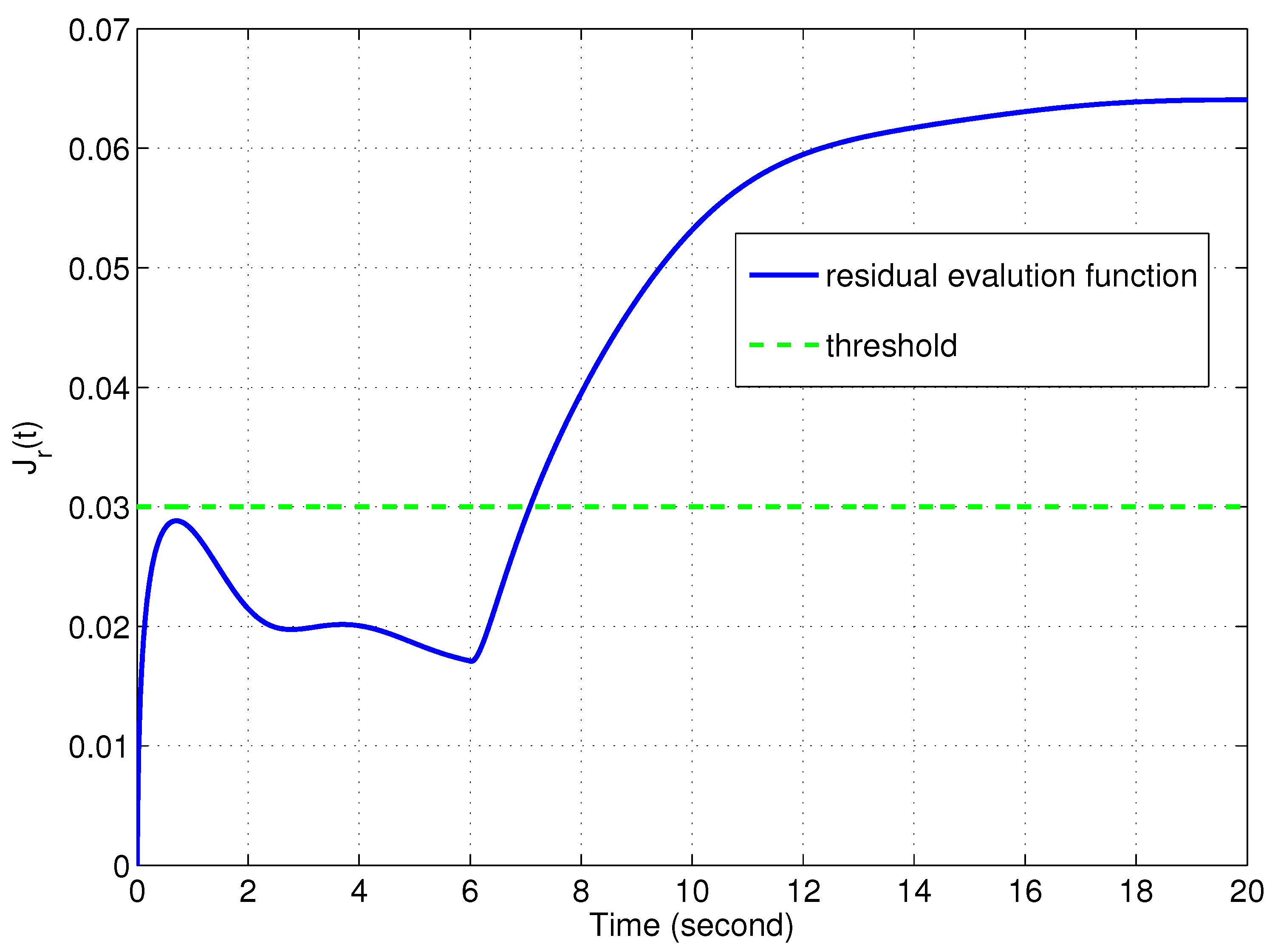
Aimed at fault detection, a widely used method is as follows. First, we define a threshold and use the logic unit, and then follow the results in [45]. Based on the above, we can define the residual evaluation function as follows:
where t represents the detection time range. We determine the threshold by
and faults can be detected by
5. Examples
In this section, we will show the effectiveness of the proposed approach with two examples. The first example aims to compare the proposed method with existing results. The second example is used to demonstrate the proposed method’s capabilities and effectiveness.
5.1. Example 1
The fractional-order model of a permanent magnet synchronous motor (PMSM) velocity control system has the following form:
The ’s pseudo-state space is expressed as follows:
With the fractional order , the fractional-order system (73) can be obtained as follows:
where is the given velocity and is the feedback value. K is the gain matrix, and and are weighted values. Experimental verification is achieved through the block diagram displayed in Figure 1. For the complementary sensitivity function from w to y and the closed-loop sensitivity function from w to , we consider and . The sensitivity functions of the closed-loop system must be verified
which are equivalent to
In order to eliminate the closed-loop static error, we have to make the constraint low enough. In order to attenuate the resonance of , constraint is chosen. The transfer function is
For system (1) without an actuator fault, we consider the general control configuration of this problem.
Furthermore, we consider the PMSM velocity control system’s integer-order model as
According to (79), with an integer order , we have
In [46], a real-time PMSM velocity servo plant, the fractional-order model is identified according to the experimental tests. The fact that the fractional model is more accurate than the traditional integer-order model is substantiated, and then according to the identified fractional-order model and the traditional integer-order one, two stabilizing output feedback controllers are designed, respectively. The experimental test performance is compared to demonstrate the advantage of the proposed fractional-order model of the PMSM velocity system.
The following optimization problem is solved for the two above-mentioned models:
The performance bounds are given in Table 2 as follows:
5.2. Example 2
Consider the following fractional-order systems
with the order
The open-loop transfer function is
It is assumed that , and the measurement output .
In this paper, we investigated the fault in a limited frequency range , assuming that the disturbance belongs to a finite frequency range . To avoid high gains in terms of the observer and controller, two constraints, and , are added to the optimization problem (68). Given , , , , , and , by using the LMI toolbox in Matlab, we can solve the optimization problem (68), and we obtain . Furthermore, we finally obtain the controller and observer gains, as follows:
Then, the simulation results are given as follows. is the initial system condition and , is the initial observer condition. Moreover, the disturbance is assumed to be and the fault signal is chosen.
Figure 2 displays the residual signal . It can be found from Figure 2 that the residual signal has large discrepancies when the fault occurs. Figure 3 shows the regulation output of the augmented system (7). From Figure 3, we can see that the influence of the disturbance and fault on the output has been weakened. Furthermore, Figure 4 plots the residual evaluation function. By using a threshold test , we can effectively detect the fault at approximately .
6. Conclusions
In this paper, we study the SFDC problem in FOSs. We give the new bounded real lemma related to the FOSs’ norm so as to assess the disturbance attenuation performance. Moreover, we introduce the GKYP lemma directly to address the finite-frequency performance indexes. Then, we applied a linearizing change-of-variables and a tangent hyperplane technique to convert the design conditions into a class of LMI. Finally, the numerical examples demonstrate the proposed approach’s effectiveness. Future work will consider the fault detection problem in a finite-frequency domain for fractional-order Lipschitz non-linear systems and fractional-order singular systems.
Author Contributions
Conceptualization, H.L.; Software, C.D.; Validation, Y.L.; Formal analysis, J.L.; Data curation, C.D.; Writing—review & editing, J.L.; Supervision, Y.L.; Funding acquisition, H.L. All authors have read and agreed to the published version of the manuscript.
Funding
This work was supported in part by the National Natural Science Foundation of China under Grant No. 62003223, and in part by the Liaoning Provincial Department of Education Series Projects (“Seedling Raising” Project for Young Scientific and Technological Talents) under Grant No. JYT2020131.
Institutional Review Board Statement
Not applicable.
Informed Consent Statement
Not applicable.
Data Availability Statement
Data sharing is not applicable to this article as no datasets were generated or analyzed during the current study.
Conflicts of Interest
The authors declare no conflict of interest.
References
- Feliu-Talegon, D.; Feliu-Batlle, V. Improving the position control of a two degrees of freedom robotic sensing antenna using fractional-order controllers. Int. J. Control 2017, 90, 1256–1281. [Google Scholar] [CrossRef]
- Monje, C.A.; Chen, Y.; Vinagre, B.M.; Xue, D.; Feliu-Batlle, V. Fractional-Order Systems and Controls: Fundamentals and Applications; Springer Science & Business Media: Berlin/Heidelberg, Germany, 2010. [Google Scholar]
- Podlubny, I. Fractional Differential Equations; Academic Press: Cambridge, MA, USA, 1999. [Google Scholar]
- Choudhary, N.; Sivaramakrishnan, J.; Kar, I.N. Sliding mode control of uncertain fractional order systems with delay. Int. J. Control 2020, 93, 934–943. [Google Scholar] [CrossRef]
- Hilfer, R. Applications of Fractional Calculus in Physics; World Scientific: Singapore, 2000. [Google Scholar]
- Kilbas, A.A.; Srivastava, H.M.; Trujillo, J.J. Theory and Applications of Fractional Differential Equations; Elsevier: Amsterdam, The Netherlands, 2006. [Google Scholar]
- Lu, J.G.; Chen, Y.Q. Robust stability and stabilization of fractional-order interval systems with the fractional order α: The 0 < α < 1 Case. IEEE Trans. Autom. Control 2010, 55, 152–158. [Google Scholar]
- Soorki, M.N.; Tavazoei, M.S. Asymptotic swarm stability of fractional-order swarm systems in the presence of uniform time-delays. Int. J. Control 2017, 90, 1182–1191. [Google Scholar] [CrossRef]
- Wei, Y. Time-varying Lyapunov functions for nonautonomous nabla fractional order systems. ISA Trans. 2021, 126, 235–241. [Google Scholar] [CrossRef] [PubMed]
- Ibrir, S.; Bettayeb, M. New sufficient conditions for observer-based control of fractional-order uncertain systems. Automatica 2015, 59, 216–223. [Google Scholar] [CrossRef]
- Lu, J.G.; Chen, G. Robust stability and stabilization of fractional-order interval systems: An LMI approach. IEEE Trans. Autom. Control 2009, 54, 1294–1299. [Google Scholar]
- Lan, Y.H.; Huang, H.X.; Zhou, Y. Observer-based robust control of α (1 < α < 2) fractional-order uncertain systems: A linear matrix inequality approach. IET Control Theory Appl. 2012, 6, 229–234. [Google Scholar]
- Boukal, Y.; Darouach, M.; Zasadzinski, M.; Radhy, N. Robust H∞ observer-based control of fractional-order systems with gain parametrization. IEEE Trans. Autom. Control 2017, 62, 5710–5723. [Google Scholar] [CrossRef]
- Farges, C.; Fadiga, L.; Sabatier, J. H∞ analysis and control of commensurate fractional order systems. Mechatronics 2013, 23, 772–780. [Google Scholar] [CrossRef]
- Shen, J.; Lam, J. State feedback H∞ control of commensurate fractional-order systems. Int. J. Syst. Sci. 2014, 45, 363–372. [Google Scholar] [CrossRef]
- Oustaloup, A.; Moreau, X.; Nouillant, M. The CRONE suspension. Control Eng. Pract. 1996, 4, 1101–1108. [Google Scholar] [CrossRef]
- Raynaud, H.F.; Zerganoh, A. State-space representation for fractional order controllers. Automatica 2000, 36, 1017–1021. [Google Scholar] [CrossRef]
- Deng, C.; Yang, G.H. Distributed adaptive fault-tolerant control approach to cooperative output regulation for linear multi-agent systems. Automatica 2019, 103, 62–68. [Google Scholar] [CrossRef]
- Fan, Q.Y.; Yang, G.H.; Ye, D. Adaptive tracking control for a class of Markovian jump systems with time-varying delay and actuator faults. J. Frankl. Inst. 2015, 352, 1979–2001. [Google Scholar] [CrossRef]
- Ye, D.; Chen, M.M.; Yang, H.J. Distributed adaptive event-triggered fault-tolerant consensus of multiagent systems with general linear dynamics. IEEE Trans. Cybern. 2019, 49, 757–767. [Google Scholar] [CrossRef]
- Liu, J.; Wang, J.L.; Yang, G.H. An LMI approach to minimum sensitivity analysis with application to fault detection. Automatica 2005, 41, 1995–2004. [Google Scholar] [CrossRef]
- Liu, N.; Zhou, K. Optimal solutions to multi-objective robust fault detection problems. In Proceedings of the 2007 46th IEEE Conference on Decision and Control, New Orleans, LA, USA, 12–14 December 2007; pp. 981–988. [Google Scholar]
- Henry, D.; Zolghadri, A. Design and analysis of robust residual generators for systems under feedback control. Automatica 2005, 41, 251–264. [Google Scholar] [CrossRef]
- Wang, H.; Wang, J.; Lam, J. An optimization approach for worst-case fault detection observer design. In Proceedings of the 2004 American Control Conference, Boston, MA, USA, 30 June–2 July 2004; pp. 2475–2480. [Google Scholar]
- Iwasaki, T.; Hara, S. Generalized KYP lemma: Unified frequency domain inequalities with design applications. IEEE Trans. Autom. Control 2005, 50, 41–59. [Google Scholar] [CrossRef]
- Gao, H.; Li, X. H∞ filtering for discrete-time state-delayed systems with finite frequency specifications. IEEE Trans. Autom. Control 2011, 56, 2932–2941. [Google Scholar] [CrossRef]
- Li, X.; Yang, G. Fault detection in finite frequency domain for Takagi-Sugeno fuzzy systems with sensor faults. IEEE Trans. Cybern. 2014, 44, 1446–1458. [Google Scholar] [CrossRef] [PubMed]
- Wang, H.; Song, W.; Liang, Y.; Li, Q.; Liang, D. Observer-based finite frequency H∞ state-feedback control for autonomous ground vehicles. ISA Trans. 2021, 121, 75–85. [Google Scholar] [CrossRef] [PubMed]
- Davoodi, M.; Meskin, N.; Khorasani, K. Simultaneous fault detection and consensus control design for a network of multi-agent systems. Automatica 2016, 66, 185–194. [Google Scholar] [CrossRef]
- Wang, S.; Jiang, Y.; Li, Y.; Liu, D. Fault detection and control co-design for discrete-time delayed fuzzy networked control systems subject to quantization and multiple packet dropouts. Fuzzy Sets Syst. 2017, 306, 1–25. [Google Scholar] [CrossRef]
- Zhai, D.; An, L.; Dong, J.; Zhang, Q. Simultaneous H2/H∞ fault detection and control for networked systems with application to forging equipment. Signal Process. 2016, 125, 203–215. [Google Scholar] [CrossRef]
- Shen, H.; Song, X.; Wang, Z. Robust fault-tolerant control of uncertain fractional-order systems against actuator faults. IET Control Theory Appl. 2013, 7, 1233–1241. [Google Scholar] [CrossRef]
- Sakthivel, R.; Ahn, C.K.; Joby, M. Fault-tolerant resilient control for fuzzy fractional order systems. IEEE Trans. Syst. Man Cybern. Syst. 2018, 49, 1797–1805. [Google Scholar] [CrossRef]
- Melendez-Vazquez, F.; Martinez-Fuentes, O.; Martinez-Guerra, R. Fractional fault-tolerant dynamical controller for a class of commensurate-order fractional systems. Int. J. Syst. Sci. 2018, 49, 196–210. [Google Scholar] [CrossRef]
- Pisano, A.; Rapaić, M.R.; Usai, E.; Jelicic, Z. Second-order sliding mode approaches to disturbance estimation and fault detection in fractional-order systems. IFAC Proc. Vol. 2011, 44, 2436–2441. [Google Scholar] [CrossRef]
- Zhong, W.; Lu, J.; Miao, Y. Fault detection observer design for fractional-order systems. In Proceedings of the 2017 29th Chinese Control And Decision Conference, Chongqing, China, 28–30 May 2017; pp. 2796–2801. [Google Scholar]
- Wang, C.; Li, H.; Chen, Y. H∞ output feedback control of linear time-invariant fractional-order systems over finite frequency range. IEEE/CAA J. Autom. Sin. 2016, 3, 304–310. [Google Scholar]
- Golabi, A.; Beheshti, M.T.H.; Asemani, M.H. Dynamic observer-based controllers for linear uncertain systems. J. Control Theory Appl. 2013, 11, 193–199. [Google Scholar] [CrossRef]
- Li, X.J.; Yang, G.H. Dynamic observer-based robust control and fault detection for linear systems. IET Control Theory Appl. 2012, 6, 2657–2666. [Google Scholar] [CrossRef]
- Park, J.K.; Shin, D.R.; Chung, T.M. Dynamic observers for linear time-invariant systems. Automatica 2002, 38, 1083–1087. [Google Scholar] [CrossRef]
- Li, J.; Pan, K.; Su, Q. Sensor fault detection and estimation for switched power electronics systems based on sliding mode observer. Appl. Math. Comput. 2019, 353, 282–294. [Google Scholar] [CrossRef]
- Li, H.; Yang, G.H. Dynamic output feedback H∞ control for fractional-order linear uncertain systems with actuator faults. J. Frankl. Inst. 2019, 356, 4442–4466. [Google Scholar] [CrossRef]
- Gahinet, P.; Apkarian, P. A linear matrix inequality approach to H∞ control. Int. J. Robust Nonlinear Control 1994, 4, 421–448. [Google Scholar] [CrossRef]
- Li, X.J.; Yang, G.H. Fault detection in finite frequency domains for multi-delay uncertain systems with application to ground vehicle. Int. J. Robust Nonlinear Control 2015, 25, 3780–3798. [Google Scholar] [CrossRef]
- Frank, P.M.; Ding, X. Survey of robust residual generation and evaluation methods in observer-based fault detection systems. J. Process Control 1997, 7, 403–424. [Google Scholar] [CrossRef]
- Yu, W.; Luo, Y.; Chen, Y.; Pi, Y. Frequency domain modelling and control of fractional-order system for permanent magnet synchronous motor velocity servo system. IET Control Theory Appl. 2016, 10, 136–143. [Google Scholar] [CrossRef] [Green Version]
Figure 1.
Block diagram of the experimental validation.
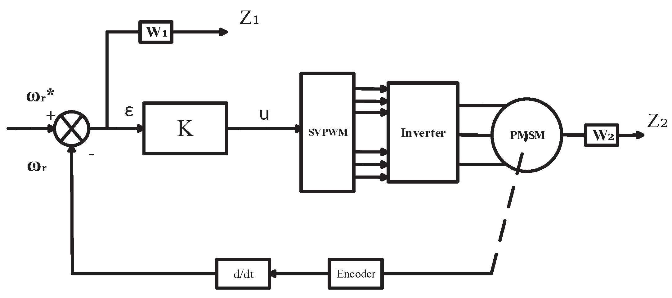
Figure 2.
Residual output .

Figure 3.
The performance output of the augmented system.
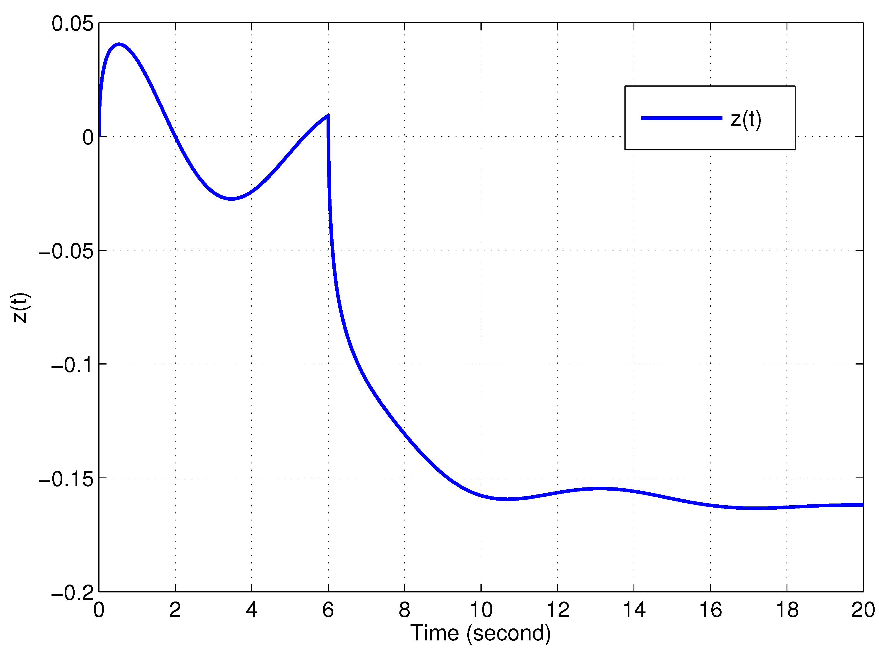
Figure 4.
Dashed line: threshold; solid line: residual evaluation function.

Table 1.
Different limited frequency ranges.
| LF | MF | HF | |
|---|---|---|---|
Table 2.
Comparison of the performance .
| Fractional Order | Integer Order | |
|---|---|---|
| 4.0339 | 4.0366 |
Disclaimer/Publisher’s Note: The statements, opinions and data contained in all publications are solely those of the individual author(s) and contributor(s) and not of MDPI and/or the editor(s). MDPI and/or the editor(s) disclaim responsibility for any injury to people or property resulting from any ideas, methods, instructions or products referred to in the content. |
© 2023 by the authors. Licensee MDPI, Basel, Switzerland. This article is an open access article distributed under the terms and conditions of the Creative Commons Attribution (CC BY) license (https://creativecommons.org/licenses/by/4.0/).
Share and Cite
MDPI and ACS Style
Li, H.; Li, J.; Deng, C.; Li, Y. Fault Detection and Reliable Controller Design for Fractional-Order Systems Based on Dynamic Observer. Actuators 2023, 12, 255. https://doi.org/10.3390/act12060255
AMA Style
Li H, Li J, Deng C, Li Y. Fault Detection and Reliable Controller Design for Fractional-Order Systems Based on Dynamic Observer. Actuators. 2023; 12(6):255. https://doi.org/10.3390/act12060255
Chicago/Turabian StyleLi, He, Jie Li, Chao Deng, and Yuanxin Li. 2023. "Fault Detection and Reliable Controller Design for Fractional-Order Systems Based on Dynamic Observer" Actuators 12, no. 6: 255. https://doi.org/10.3390/act12060255
Note that from the first issue of 2016, this journal uses article numbers instead of page numbers. See further details here.