
Modeling and Clamping Force Tracking Control of an Integrated Electric Parking Brake System Using Sliding-Mode-Based Observer

1
Department of Traffic Engineering, Beijing University of Technology, Beijing 100124, China
2
State Key Laboratory of Automotive Safety and Energy, Tsinghua University, Beijing 100084, China
3
Trinova-Tech Co., Ltd., Tianjin 301701, China
*
Author to whom correspondence should be addressed.
Actuators 2024, 13(1), 39; https://doi.org/10.3390/act13010039
Submission received: 3 December 2023
/
Revised: 12 January 2024
/
Accepted: 12 January 2024
/
Published: 17 January 2024
(This article belongs to the Section Actuators for Land Transport)
Abstract
:This article proposes a hierarchical control strategy to address semi-ABS control as well as the precise clamping force control problems for an integrated electric parking brake (iEPB) system. To this end, a detailed system model, including modeling of the motor, transmission mechanism, friction and braking torque, is constructed for controller and observer design, and a sliding-mode-based observer (SMO) is proposed to estimate the load torque by using the motor rotational speed without installing a force sensor. In addition, a stable and reliable tire–road friction coefficient (TRFC) estimation method is adopted, and the desired slip ratio (DSR) is observed as the target that the rear wheels cycle around. At the upper level of the hierarchical control structure, the desired clamping forces of the rear wheels are generated using a sliding mode control (SMC) technique, and the control objective is to track the DSR to make full use of the road condition. At the lower level, the motor is controlled to track the desired clamping force generated from the upper controller. The hardware-in-the-loop (HIL) experimental results demonstrate the effectiveness and high tracking precision of the proposed strategy under different road conditions, and the estimation parameters based on the proposed observers are timely and accurate to satisfy the control requirements.
1. Introduction
An iEPB system achieves better performance in terms of its fast response and active function in contrast to traditional parking brake systems [1,2], and it will dominate the parking brake market in the future. In addition to the parking brake function, an iEPB system could also implement a secondary braking function if the primary braking system fails, or it could realize active safety functions by regulating the clamping forces. However, for active safety function applications, the regulation of the clamping forces will cause a risk of the vehicle spinning if the iEPB is applied without slip ratio control, especially on low-adhesion-coefficient surfaces. Therefore, to ensure the vehicle stability during conditions with an applied active safety function, the slip ratio of iEPB-equipped wheels should be controlled precisely and steadily to track the DSR based on the vehicle’s system dynamics [3,4].
The slip ratio reveals the maximum adhesion forces that the road can provide, both in the longitudinal and lateral directions, and it is also adopted as an indicator of the wheel-locking status. Many methods have been proposed to address the slip ratio control problem [4,5,6,7,8], and the algorithms should normally have two features: (1) an optimal slip ratio should firstly be estimated with different road conditions, and (2) a controller should be designed to control the slip ratio following the optimal one for improving the stability and security performance of the vehicle during acceleration/braking situations. Note that the TRFC is critical in determining the optimal slip ratio, so a high-precision TRFC observer should be first developed. Although the accuracy of these TRFC observers [9,10,11] has been verified by simulations and experiments, they are too complex, and the associated complicated computation requirements will significantly decrease the executing efficiency of the micro-controller chip (MCU) integrated in the vehicle’s electric control unit (ECU). Hence, a practical and effective observer should be proposed that can be properly utilized in practical control situations with a low-cost MCU.
The control of a direct-current (DC) motor is complicated because of the presence of disturbances, measurement noise and load torque perturbations, which have promoted research into observer-based sensorless control. Ref. [12] presented a new extended nonlinear approach to estimate the motor speed and load torque simultaneously, and an augmented dynamical system was created by affiliating a supplementary dynamic into the motor model to admit changes in coordinates. However, the performance of the method depends on the model’s accuracy and system parameters. Sliding-mode-based methods and observers have been studied in recent years, and they benefit from their insensitivity to parameter variations and disturbances [13,14,15]. Ref. [16] regarded system inertia and friction and designed an SMC-based load torque estimation method. Ref. [17] proposed a motor speed and torque observer with consideration of electrical and mechanical parameter disturbances and the voltage reconstruction error as well. To eliminate the chattering problem, ref. [18] deduced and analyzed the mathematical model of a traditional SMC-based load torque identification observer, and a new one was designed by employing a saturation function instead of the sign one. However, this method requires an offline table, which is generated from experimental results, for parameter optimization and disturbance compensation, and this will limit the identification accuracy, especially in high-speed conditions. Some other studies into the load torque estimation of different actuators are also helpful for motor load torque observation [19,20,21].
With the above observers, an iEPB system should be quickly and precisely operated over a wide range of clamping forces to meet the requirements, whether from the driver or from the upper controllers as a brake-by-wire system. Ref. [22] proposed a nonlinear proportional clamping force controller for an electric parking system using the measured clamping force to improve the control performance based on a state-independent switched system model. However, it is too expensive to install an embedded clamping force sensor in production vehicles, and the measurement accuracy at high temperatures is also a worrying aspect. To solve these problems, observers should seek to estimate the clamping force without measurement sensors. Ref. [23] estimated the clamping force through the angular displacement of a DC motor and approximated the initial contact point using the motor angular velocity to prevent the error caused by the gap between the brake pad and disk at release, whereas the estimation precision was affected by the age and temperature of the contact point. In [24,25], the clamping force control methods used for an electro-mechanical brake system are studied, and these could also be applicable for an iEPB after a few modifications.
The above studies have acquired many achievements in improving the control performance of iEPB systems. However, it is still a big challenge to comprehensively and precisely control the clamping force of an iEPB to realize active braking functions. In this paper, a hierarchical control strategy to address semi-ABS control as well as the precise clamping force control problems for an iEPB system are proposed, which provide the potential for iEPB systems to be applied in active braking control or even in implementing a secondary braking function if the primary braking system fails. To this end, an eight-degrees-of-freedom nonlinear vehicle model, a tire model and a detailed iEPB system model are established for controller design and parameter observation. Meanwhile, a stable and reliable TRFC observation method is adopted to estimate the TRFC and DSR, and an SMO is proposed to estimate the load torque by using the motor rotational speed without installing a force sensor. Furthermore, a hierarchical control structure, which contains an upper controller to track the DSR to realize semi-ABS function and a lower controller to track the desired clamping force based on the SMO, is designed. Finally, numerical experiments are carried out on an HIL test bench to evaluate the proposed algorithm.
The rest of the paper is organized as follows: in Section 2, the involved models are established, including a vehicle model, a tire model and an iEPB system model. An SMC-based observer for motor load torque estimation is presented in Section 3. Section 4 describes the semi-ABS and clamping force control strategies. HIL experimental results are presented to discuss the performance of the proposed algorithm in Section 5. Conclusions are given in the end.
2. System Modeling
In this section, an eight-degrees-of-freedom (8-DOF) nonlinear vehicle model and tire model are presented for simulation and parameter estimation; a control-oriented iEPB system model, including a DC motor model, a transmission mechanism model, a brake model, a screw-nut model and a caliper model, is proposed for controller design.
2.1. Vehicle Model
The governing equations of motions of the sprung mass can be expressed as shown below [26,27]:
where m represents the vehicle mass. u and va stand for the longitudinal and lateral velocities, respectively. r denotes the yaw rate. mφ is the vehicle sprung mass. hφ stands for the height of the center of roll part gravity with respect to (WRT) the roll axis. φ denotes the roll angle around the roll axis. θr indicates the inclination angle of the roll axis WRT horizontal plane. Cφ describes the total roll stiffness. Iz represents the yaw moment of inertia around the z-axis. Ixφ, Iyφ and Izφ stand for the rotational inertias of sprung mass around the x-axis, y-axis and z-axis, respectively. Qu, Qr, Qφand Qv represent the general forces of the x-axis, y-axis, yaw motion and roll motion, respectively.
where F expresses the tire forces, the subscripts x and y indicate the x-axis and y-axis, respectively, and the subscripts 11, 12, 21 and 22 denote the front-left, front-right, rear-left and rear-right wheel; accordingly, these subscripts represent the same definition in the following appearance. Δ is the total applied steer angle, tw is the wheel track, and a and b are the horizontal distances from the center of gravity to the front and rear axles, respectively. kφ1 and kφ2 represent the roll damping coefficients of the front and rear axles, respectively.
The vertical load transfer occurs during acceleration or deceleration situations, and is can be expressed as follows:
in which Fz and Fzs indicate the vertical dynamic and static forces on wheels, L denotes the wheelbase, ij represents 11, 12, 21, and 22. In addition, + and − need to be properly selected for different wheels. It is assumed that the lateral inertia force is located on four wheels equally in this paper.
The rotational motions of wheels are as follows:
in which Jf and Jr denote the rotational inertias of the front and rear wheels, respectively. Rf and Rr are the radiuses of the front and rear wheels, accordingly. Tb is the hydraulic braking torque of different wheels. Tepb is the braking torque of rear wheels applied from the iEPB system, and Tw is the driving torque of different wheels.
2.2. Tire Model
The nonlinear Dugoff tire model defines the longitudinal and lateral tire forces as shown below [28]:
In which Ck = CsFz represents the longitudinal slip stiffness of the tire, Cs indicates the normalized longitudinal slip stiffness of the tire, α is the slip angle, s denotes the slip ratio, and κ and are determined by
where μ denotes the nominal TRFC.
The major advantage of the Dugoff model is that the tire stiffness can be divided into longitudinal and lateral directions independently. However, different from the Magic Formula tire model, the precision of the Dugoff model drops significantly when the slip ratio is larger than 0.3 [28]. A modified Dugoff tire model is proposed to settle this issue. The pure longitudinal and lateral TRFCs are defined as shown below:
where μxp and μyp are the peak value of the longitudinal and lateral TRFCs, respectively. μxs and μys represent the longitudinal and lateral sliding TRFCs, respectively. Ss and Sα are defined as
The slip ratio is redefined to ensure positive results even in braking conditions:
2.3. Structure and DC Motor Model of the iEPB
The iEPB actuator consists of a DC motor, a belt drive, a gear reducer, a ball-screw assembly, a caliper, two friction pads, a piston, and an ECU to execute the lower-level algorithm. Two of the same iEPB actuators are installed separately in the left and right rear wheels, and an overall ECU is adopted to execute the upper-level algorithm to generate the desired clamping forces for both rear wheels. The DC motor affects the clamping force generation or regulation characteristics significantly, and the electrical equations of the DC motor are as follows:
in which ua denotes the pulse width modulation (PWM) duty, Va is the motor nominal voltage, ia represents the motor current, and ωm is the motor rotational speed. Eb and ke represent the counter electromotive voltage and constant, respectively. La and Ra indicate the phase-to-phase terminal inductance and resistance, accordingly. The system torque balance equations are described as follows:
where Jm represents the motor rotational inertia, Ta is the motor electromagnetic torque, Tm denotes the load torque applied to the motor shaft, cm stands for the motor damping coefficient, and kt is the torque constant.
2.4. Screw-Nut and Caliper Mechanism Model
The screw rotates to move the nut forward or backward in the axial direction to regulate the clamping forces, and it can be described as
where θs denotes the screw rotational angle, snut stands for the nut stroke, and Ph indicates the screw-nut pitch.
For precisely building the screw-nut model, the motion of the screw-nut assembly has been regarded as a slide block that moves along an inclined surface, as shown in Figure 1. d1 and d2 represent the inside and outside diameters of the screw, respectively, γ denotes the thread angle, FN indicates the normal force, FQ (clamping force) and FH stand for the normal force distributed along the axial and radial directions, respectively, and vs is the nut linear speed along with the inclined surface.
The force balance expressions are derived
where Tscew stands for the screw driving torque, d denotes the medium diameter of the screw, Ffs is the friction force before the maximum static friction fs has been overcome, Ffc represents the Coulomb friction force, and μs indicates the sliding friction coefficient.
The friction force generated by the contact surface inside the screw-nut assembly will affect the clamping force tracking performance significantly. Therefore, this paper concentrates on the static, Coulomb, viscous and Stribeck effects, and a simplified friction model is generated based on the Tustin model to improve control accuracy [29].
in which Ff denotes the total friction force, fv is the viscous friction coefficient, and vst stands for the Stribeck speed.
Figure 2 shows the Tustin friction curve and simplified fitting lines proposed in this paper. and are the intersection points of lines in positive and negative velocity regions, respectively. The slopes of the lines Lp1, Lp2, Ln1, Ln2 are decided by , , , and , accordingly. vpmax and vnmax represent the maximum positive and negative velocities of the nut. Together with the points , , and , the lines can be expressed as follows:
Equation (25) could be further simplified as
The parameters of the friction model had been identified through numerical experiments on an HIL test platform, and the nut moving speed was controlled to change from −50 to 50 mm/s with a resolution of 2 mm/s. Four lines were fitted through the experiment results employing the least square method, and the finally identified parameters are listed in Table 1.
2.5. Control-Oriented Transmission Mechanism Model
The mechanical diagram of the iEPB actuator is shown in Figure 3. Here, 1 and 2 indicate the driving and driven pulleys of the belt drive, respectively, while 3, 4 and 5 represent the sun gear, planet gear and planet carrier of the first planetary gear set, respectively. The numbers 6, 7 and 8 denote the sun gear, planet gear and planet carrier of the second planetary gear set, respectively, while 11 is the ring gear for both of the two planetary gear sets. The numbers 9 and 10 indicate the screw and nut of the ball-screw assembly. Lastly, 12, 13 and 14 are the pad, disc, and caliper, respectively. When parking or other active braking functions are requested, the gap between the pad and disc will be overcome firstly, and then the clamping force is generated.
When the braking function is applied, the dynamic motions of the iEPB system are described as follows:
When the braking function is released, the dynamic motions of the iEPB system can be expressed by the following equations
where T, Jtm, ωtm, mtm, and rtm stand for the torque, inertia, rotational speed, mass and radius of corresponding components, respectively, and the numerical subscripts stand for the corresponding components shown in Figure 3. ηtm and itm denote the transmission efficiency and ratio from the component corresponding to the first subscript to the component corresponding to the second subscript. N is the number of the planetary gears, while ctm1, ctm2, and ctm3 are the rotational damping coefficients of shaft-bearings of the driving pulley, driven pulley and second planet carrier, respectively.
The rotational speed equations are as follows:
where Z is the teeth number of corresponding components. According to Equations (27)–(29), the equivalent rotational damping coefficient ceq and the equivalent inertia Jeq are determined by
where , .
Combining Equations (27)–(31), after some manipulations, we have
in which Tr stands for the resistance torque at the motor shaft. Considering Equations (20), (21) and (32), we have
where
2.6. Brake Model
The braking torque can be defined in terms of the clamping force as
where μb represents the friction coefficient between the pad and disc, and rp denotes the equivalent radius from the pad to the disc center.
3. Sliding-Mode-Based Load Torque Observer
If the request braking deceleration exceeds the maximum force that the surface can provide, an ABS function should be triggered to maintain the vehicle stability and to shorten the braking distance. Therefore, we assume that the proposed strategy is used for realizing a semi-ABS function of the two rear wheels. A hierarchical control structure is designed, as shown in Figure 4. For realizing sensorless control of the lower level, an observer should be designed to estimate the load torque of the motor, and the estimation value will be adopted as the actual motor torque to achieve a closed-loop control of the motor.
The main sensitive parameters that affect the observer accuracy include the motor current ia, the phase-to-phase terminal inductance La, the phase-to-phase terminal resistance Ra and the motor rotational speed ωm. The execution cycle of the ECU, which is set to a frequency of 1 kHz in this paper, is very transient, and the load torque varies very slowly. Therefore, it is assumed that the load torque (or ia) is non-variable within one control cycle [30]. La and Ra are reflected by Equation (20); ωm is designed as the observation object. The dynamic equations of the DC motor, which is shown in Equations (33) and (34), can be converted into
The rotational speed and load torque-tracking errors are defined as follows:
where and stand for the estimated rotational speed load torque, respectively. Shown in Equation (37) is a first-order control system, and the sliding surface is designed in terms of speed-tracking error
Since the transfer function of Equation (39) is stable (H(s) = 1), if the sliding surface is controlled to remain small or converge to zero, then the tracking error e1 will be adjusted to a small range. The SMO for rotational speed and load torque estimation is designed as
where g is the feedback gain, and U is the control law. A piecewise linear approximation saturation function is adopted to eliminate the chattering problem as follows [31]:
where is the thickness of the boundary layer, K > 0 is the sliding-mode gain, and
Substituting Equation (40) into Equation (38), after some manipulations, we have
The following Lyapunov function is defined to discuss the stability of the SMO.
Thus,
Considering Equations (39), (41) and (43), after some manipulations, we have
Apparently, , and the expression in the bracket should be nonnegative to ensure the stability of the controller. Thus, the sliding-mode gain is determined by
If we assume that the tracking errors e1 and e2 are separately positive and negative, Equation (47) could be further expressed as
According to Equation (46), s will arrive at the sliding surface within a limited time if we assume that the beginning error e1(0) is finite, and therefore the speed-tracking error e1 will converge to 0 when the proposed SMO falls into the surface. When e1 = 0, Equation (43) could be further simplified as
Thus, the load torque observation error is determined by
in which C is a constant, and t is the total observation time. g/Jt should be negative for adjusting e2 to converge to zero. To this effect, g will determine the attenuation rate of e2, and it has to be negative.
4. Hierarchical Semi-ABS Controller Design
As shown in Figure 4, the upper controller is designed to track the DSR to fully utilize the road condition, and the desired braking torques for rear wheels are derived using the SMC technique; at the lower level, the motor is controlled to implement the desired braking torque that resulted from the upper controller. The desired clamping forces are finally obtained by Equation (36) and the braking torques, and the actual clamping forces are calculated based on the load torque estimation results and the iEPB mechanism model.
4.1. Upper Controller
The slip ratios of the rear wheels are calculated with rear wheel rotational speeds and vehicle speed, which is observed by the electronic stability control algorithm (integrated into the iEPB’s ECU). A TRFC observer is designed according to the μ-slip curve and experimental calibration parameters, and furthermore, the DSR is estimated from the characteristics of the utilized friction coefficient and the slip ratio. The upper controller is proposed to generate the desired braking torques to maintain the rear slip ratio tracking errors within a small range or converged to zero.
For both two rear wheels, the slip ratio-tracking error er is determined by the actual one λr and the desired one λrd as
The sliding surface sr is designed as
where C1 is a positive coefficient. Since the transfer function is stable, the tracking error er will converge to 0 if the sliding surface is controlled to converge to 0.
The first derivative of sr is derived as follows:
The reaching law has been defined in terms of a piecewise linear approximation saturation function as
where ε1, ε2 are positive sliding-mode gain factors, and is the thickness of the boundary layer. has the same definition as shown in Equation (42).
It is assumed that the hydraulic braking is not activated, which means that Tbr is equal to 0. With Equations (5), (10) and (19), after some manipulations, we have
Substituting Equation (55) into Equation (53), yields
The control law is defined as
The Lyapunov function is designed as
Thus,
According to the assumptions and Equation (59), the upper controller is stable and sr will arrive the sliding surface within a limited time if we assume that the beginning error er(0) is finite, and then a continuous function is adopted to eliminate the chattering problem when inside the boundary layer . It is assumed that Equation (59) holds until , and , which is determined by the system disturbances, is the thickness of the thinnest boundary layer. The price for eliminating chattering and achieving a smooth control law is a loss of precision, and the ensured accuracy is decided by , where Cct is the constant of integration, and t is the total convergence time.
4.2. Lower Controller
The main sensitive parameters that affect the lower control performance include the motor load torque, the mechanical transmission, the mechanical friction and the disturbances. The load torque is estimated by the proposed observer, and the detail control-oriented mechanical transmission model is established in Section 2.5. The mechanical friction characteristics is simplified into four fitting lines to create an online friction estimation model, as illustrated in Section 2.4. An SMC-based braking torque controller, which is insensitive to disturbances and uncertainties, is proposed in lower level, by which the actual braking torque will be adjusted to follow the desired one generated from the upper level; the actual braking torque is calculated by the designed SMO. The motor terminal inductance La is very small, and it is assumed to be negligible; the braking torque can be described with Equations (20), (33), (34) and (36)
and
We define the braking torque-tracking error as follows:
where Tepbrd stands for the desired braking torque, and the sliding surface ST is defined as
where C2 is a positive constant; deriving Equation (63) WRT time, we have
The reaching law is designed as follows:
where ε3 and ε4 are positive sliding-mode gain factors, and is the thickness of the boundary layer. Substituting Equation (60) into Equation (64), after some manipulations, yields
The control law is defined as
The Lyapunov function is designed as
Deriving Equation (68), considering Equation (65), we have
5. Experimental Test and Analysis
The proposed algorithm is evaluated in this section through realizing semi-ABS functions. To this end, firstly, a real-time HIL test bench installed with iEPB prototypes was developed. Subsequently, a lot of vehicle dynamic experiments, including single-lane-change, double-lane-change, steady-state cornering, step response, pylon course slalom, transition brake and split brake maneuvers, were conducted to calibrate the vehicle model, and the final adjusted parameters were derived to enhance the model accuracy using the experimental results. Ultimately, semi-ABS experiments were conducted on the real-time HIL test bench to evaluate the effectiveness and accuracy of the presented controller.
5.1. HIL Test Bench Design
Figure 5 shows the HIL test bench. The industrial personal computer (IPC) runs TASS International PreSCAN 8.5.0 to provide experimental animation and environmental sensing data. The operation monitor displays the experimental data and the maneuver configuration options, and the scenario monitor is used to display the experimental animation. The dSPACE SCALEXIO is employed to run the vehicle model in real time and to sample signals from underlying actuators. The T-Booster actuator, which generates hydraulic braking pressure with an electric motor and a transmission mechanism, is adopted to amplify the driver’s brake effort or to realize active braking functions in special conditions. The EPS actuator can amplify the driver’s steering effort and implement active steering control. The proposed algorithm code is generated from the MATLAB/Simulink block diagrams, and the generated code is downloaded to the ECU that includes a low-cost MCU, NXP SPC5744, several communication and power amplifier chips. The MCU executes the proposed algorithm for iEPB prototype control and samples signals at a rate of 1 kHz.
5.2. Vehicle Model Validation and Modification
The JAC iEV7S model, which is a four-wheel double-drive electric passenger car produced by a Chinese automotive manufacturing company named Anhui Jianghuai Automobile Co., Ltd., was firstly employed for vehicle model calibration. Furthermore, experimental devices were installed inside or outside the dynamic test vehicle as shown in Figure 6, and various dynamic experiments under different maneuvers were carried out. Ultimately, the vehicle model was modified with the test results, and a set of finely tuned parameters of the vehicle model were determined, as shown in Table 2.
The lateral acceleration and yaw rate, which are the two most essential factors to reveal body stability during manipulating the vehicle, are selected to give a comprehensive judgement between the experimental and simulation results. Figure 7 shows the test and simulation results under the pylon course slalom maneuver. The root-mean-square (RMS) error of lateral acceleration between the experiment and simulation is 0.08 m/s2, whereas that of the yaw rate is 0.01 rad; the vehicle model’s accuracy reflected by lateral acceleration and yaw rate is 98% and 95%, respectively. Thus, the modified vehicle model can precisely reflect the vehicle dynamics and it is reasonable for it to be employed in the real-time HIL experiments.
5.3. Experimental Validation of the Load Torque Observer
Experiments were conducted to validate whether the designed observer is effective. The motor target rotational speed is 300 rad/s, and the motor is abruptly loaded and unloaded at run time. As shown in Figure 8, the estimated load torque matches very well with the actual one, although the usage of low accuracy encoder leads to a large rotational speed measurement error. This indicates that the proposed observer is effective and robust in dealing with signal fluctuations.
5.4. Experiment Results and Analysis of the Proposed Controller
Numerical experiments were carried out on the HIL test bench to evaluate the proposed algorithm under homogenous surface, transition surface and split surface maneuvers.
5.4.1. Straight-line Braking on High-μ Homogeneous Surface
Figure 9 indicates the results achieved under the straight-line braking on a homogeneous surface maneuver at a longitudinal velocity of 100 km/h and with a high TRFC of 0.8. Figure 9(1) shows the actual and estimated TRFCs; the estimated TRFC can track the actual one well and quick, and the steady-state error (SSE) is under 0.03. However, the TRFC observer is designed according to the μ-slip experience curve, and the curve is divided into three regions to derive corresponding simplified expressions using different slope ranges, and the slope ranges, which are calibrated by road experiments, may vary slightly on different road surfaces. These tiny parameter errors will lead to a decrease in the accuracy of the observer, especially on a high-μ surface. As shown in Figure 9(1), the estimation error is increased after about 19 s. Nevertheless, the estimation error is within a reasonable range for the proposed controller.
The time histories of the vehicle and wheel velocities derived from the model are shown in Figure 9(2); the vehicle is well controlled with the intervention of the proposed upper controller to avoid the rear wheels from locking up. Figure 9(3) illustrates the actual slip ratios of the rear wheels to following the desired one. The controlled actual slip ratios fluctuate frequently but slightly during the whole braking maneuver to help the rear wheels remain anti-locked successfully.
Figure 9(4),(5) reveal the clamping force tracking performance of the lower controller. The desired clamping forces of the rear wheels are calculated with Equation (36) using the desired braking torque generating from the upper controller, and the actual clamping forces are estimated by the proposed SMO and the iEPB mechanism model. The actual clamping forces track the desired ones quite well without obviously fluctuation throughout the whole braking maneuver, and the RMS force tracking errors of RL and RR wheels are separately 0.19 kN and 0.35 kN.
5.4.2. Straight-Line Braking on Low-μ Homogeneous Surface
To examine the algorithm performance under different TRFCs, Figure 10 shows the results derived under straight-line braking on a homogeneous surface maneuver at a longitudinal speed of 100 km/h and with a low TRFC of 0.2. Figure 10(1) illustrates the time histories of the actual and estimated TRFCs; it achieves a better estimation performance than high TRFC maneuvers. The RMS force tracking errors of RL and RR wheels are 0.13 kN and 0.14 kN, respectively.
In most of the braking process, the clamping forces of the RL and RR wheels regulate more frequently on a low TRFC road than that on a high one. Figure 10 reveals that the clamping force increasement times of the RL and RR wheels are 31 and 38 in approximately 6 s, whereas that of Figure 9 are 14 and 19 in about 4 s. As indicated in Figure 10(3), the slip ratios of RL and RR wheels change quickly due to regulation of clamping forces, which could be clearly seen when the clamping forces are decreased at about 9.8 s and 21.8 s. Although the slip ratio changes dramatically owing to the clamping force regulation, it is within a reasonable range, which always keeps the wheels in anti-lock status, as illustrated in Figure 10(2).
5.4.3. Straight-Line Braking on μ-Jump Surface
Straight-line braking under a low-to-high μ surface was conducted to examine the proposed algorithm under a road friction coefficient step variation maneuver. Figure 11(1) indicates the time histories of the actual TRFC and the estimated one, a small estimation overshoot occurs at the road friction coefficient step change point due to rapid tracking performance, and the SSE of estimation is less than 0.04. The vehicle and wheel velocities generated on this maneuver are presented in Figure 11(2); the vehicle velocity reduces slowly, while the wheel velocities drop faster on a low adhesion coefficient surface before 9.4 s, and then the vehicle velocity decreases fast. As a result, the road adhesion coefficient suddenly increases to 0.8 after 9.4 s. Since the wheels are more likely to lock up on a low-adhesion road, Figure 11(3) shows that the slip ratios derived from the low-adhesion coefficient road regulate more sharply than those generated from the high-adhesion coefficient road. Figure 11(4),(5) shows the time histories of the RL and RR clamping forces, which exhibit the clamping force tracking performance in response to adhesion coefficient step variation. The desired clamping forces have been increased on the high TRFC road after about 9.4 s, and the RMSE of the RL and RR wheels are 0.09 kN and 0.1 kN, which reveals that the proposed controller achieves sufficient clamping force tracking performance.
5.4.4. Straight-Line Braking on μ-Split Surface
Figure 12 shows the results derived from the straight-line braking on a μ-split surface maneuver at a vehicle longitudinal velocity of 50 km/h with a left-side low-μ of 0.2 and right-side high-μ of 0.8. The estimation performance in coping with TRFC variation is shown in Figure 12(1); it is indicated that the estimated TRFCs of both the left and right sides match with the actual ones very well without remarkable tracking errors throughout the whole test maneuver. A close observation of velocities and slip ratios shown in Figure 12(2),(3) reveals that the RL wheel more easily lock up on a low-μ road due to slip ratio’s dramatic fluctuations, whereas the RR wheel is not inclined to lock up on a high-μ road with a desirable slip ratio.
As shown in Figure 12(4),(5), the RMS clamping force tracking errors of the RL and RR wheels are 0.11 kN and 0.13 kN, respectively, which ensures sufficient tracking performance. The peak tracking error (PTE) occurs, at which the clamping force changes to decrease or increase, for example at the certain moments of t = 9.6 s, t = 10 s, etc. in Figure 12(4), and at the certain moments of t = 8.4 s, t = 10.8 s, etc. in Figure 12(5). Once the direction of the clamping force increase changes, which means the iEPB motor changes direction, it will give rise to a direction turning of the friction. Conversely, the direction change in friction may lead to generate PTEs.
6. Conclusions
A hierarchical control strategy was developed to address the semi-ABS control problem of the rear wheels as well as the precise clamping force control issue without a clamping force sensor. An HIL system integrated with iEPB actuators and an algorithm was established to implement real-time experiments to verify and evaluate the proposed strategy, putting particular focus on vehicle model validation and modification to enhance the model’s accuracy and thereby ensuring the reliability and validity of the HIL experiment results. The experimental results imply that the proposed SMO is effective for load torque estimation and reasonably robust in coping with signal fluctuation, the estimation error is less than 2%, and the TRFC observer can constrain the error within 5%. The semi-ABS function experimental results show that the upper controller can rapidly generate the desired clamping forces for left and right rear wheels under different road surface conditions, and the lower controller provides a satisfactory performance in terms of tracking the designed clamping forces while maintaining the fluctuation in a small range. The proposed method provides the potential for an iEPB system to implement a secondary braking function if the primary braking system fails, or to realize active braking, or even to develop an anti-lock braking control system in practice.
Nonlinear characteristics and uncertainties always existed in iEPB control systems, such as estimation errors, measurement noise and mechanical friction. The SMC-based controller has low sensitivity to plant parameter variations and uncertainties, which decreases the requirement of model accuracy. Therefore, robust SMC-based controllers are designed in this paper. However, to eliminate the chattering problem, the thinnest boundary layer, which is determined by the uncertainties, is generated by employing a continuous reaching law, and the price for eliminating chattering and achieving a smooth control law is a loss of control precision. Thus, our future work will concentrate on the further improvement of control accuracy with the consideration of uncertainties. Moreover, the iEPB system could only realize a semi-ABS function since only the two rear wheels are equipped with iEPB systems in production vehicles. Hence, our future work will also focus on the cooperative control of the proposed iEPB system and regenerative braking system or electro-hydraulic braking system [32] to implement four-wheel-ABS function.
Author Contributions
Conceptualization, J.Y. and L.L.; methodology, J.Y. and D.W.; software, J.Y. and D.W.; validation, J.Y., L.L. and D.W.; formal analysis, Y.L.; investigation, J.Y.; resources, Y.L.; data curation, J.Y and D.W.; writing—original draft preparation, J.Y.; writing—review and editing, J.Y. and L.L.; visualization, Y.L.; supervision, L.L. and Y.L.; project administration, D.W.; funding acquisition, J.Y. All authors have read and agreed to the published version of the manuscript.
Funding
This research was funded by the National Natural Science Foundation of China (No. 52002009), Beijing Natural Science Foundation (No. 3222003), and the State Key Laboratory of Automotive Safety and Energy under Project No. KF2010.
Data Availability Statement
The data that support the findings of this study are available from the corresponding author upon reasonable request.
Conflicts of Interest
Author Mr. Dongliang Wang was employed by the company Trinova-Tech Co., Ltd., Tianjin. The remaining authors declare that the research was conducted in the absence of any commercial or financial relationships that could be construed as a potential conflict of interest.
References
- Wang, B.; Guo, X.X.; Zhang, W.; Chen, Z.F. A study of an electric parking brake system for emergency braking. Int. J. Veh. Des. 2015, 67, 315–346. [Google Scholar] [CrossRef]
- Zhang, L.; Yu, W.; Zhao, X.; Meng, A.H.; Fahad, M. Force-tracking control of a novel electric parking brake actuator based on a load-sensing, continuously variable transmission. Proc. Inst. Mech. Eng. Part D J. Automob. Eng. 2016, 230, 1569–1582. [Google Scholar] [CrossRef]
- He, Z.J.; Shi, Q.; Wei, Y.J.; Gao, B.Z.; Zhu, B.; He, L. A model predictive control approach with slip ratio estimation for electric motor anti-lock braking of battery electric vehicle. IEEE Trans. Ind. Electron. 2022, 69, 9225–9234. [Google Scholar] [CrossRef]
- Jung, S.; Kim, T.; Yoo, W. Advanced slip ratio for ensuring numerical stability of low-speed driving simulation Part I: Longitudinal slip ratio. Proc. Inst. Mech. Eng. Part D J. Automob. Eng. 2019, 233, 2903–2911. [Google Scholar] [CrossRef]
- Jia, F.J.; Liu, Z.Y.; Zhou, H.J.; Chen, W. A novel design of traction control based on a piecewise-linear parameter-varying technique for electric vehicles with in-wheel motors. IEEE Trans. Veh. Technol. 2018, 67, 9324–9336. [Google Scholar] [CrossRef]
- Li, W.F.; Du, H.P.; Li, W.H. Four-wheel electric braking system configuration with new braking torque distribution strategy for improving energy recovery efficiency. IEEE Trans. Intell. Transp. Syst. 2020, 21, 87–103. [Google Scholar] [CrossRef]
- Milad, J.; Ehsan, H.; Amir, K.; Shih-ken, C.; Bakhtiar, L. A combined-slip predictive control of vehicle stability with experimental verification. Veh. Syst. Dyn. 2018, 56, 319–340. [Google Scholar]
- Li, Z.H.; Wang, P.; Liu, H.H.; Hu, Y.F.; Chen, H. Coordinated longitudinal and lateral vehicle stability control based on the combined-slip tire model in the MPC framework. Mech. Syst. Signal Process 2021, 161, 107947. [Google Scholar] [CrossRef]
- Liu, Y.H.; Li, T.; Yang, Y.Y.; Wu, J. Estimation of tire-road friction coefficient based on combined APF-IEKF and iteration algorithm. Mech. Syst. Signal Process 2017, 88, 25–35. [Google Scholar] [CrossRef]
- Hu, J.Q.; Subhash, R.; Zhang, Y.M. Real-time estimation of tire-road friction coefficient based on lateral vehicle dynamics. Proc. Inst. Mech. Eng. Part D J. Automob. Eng. 2020, 234, 2444–2457. [Google Scholar] [CrossRef]
- Feng, Y.C.; Chen, H.; Zhao, H.Y.; Zhou, H. Road tire friction coefficient estimation for four wheel drive electric vehicle based on moving optimal estimation strategy. Mech. Syst. Signal Process 2020, 139, 106416. [Google Scholar] [CrossRef]
- Ramdane, T.; Driss, B.; Zheng, G.; Frédéric, K.; Rachid, E.G. Rotor speed, load torque and parameters estimations of a permanent magnet synchronous motor using extended observer forms. IET Control Theory Appl. 2017, 11, 1485–1492. [Google Scholar]
- Kchaou, M.; Jerbi, H. Reliable H∞ and passive fuzzy observer-based sliding mode control for nonlinear descriptor systems subject to actuator failure. Int. J. Fuzzy Syst. 2022, 24, 105–120. [Google Scholar] [CrossRef]
- Kchaou, M.; Regaieg, M.A.; Al-Haijaji, A. Quantized asynchronous extended dissipative observer-based sliding mode control for Markovian jump TS fuzzy systems. J. Franklin Inst. 2022, 359, 9636–9665. [Google Scholar] [CrossRef]
- Kchaou, M.; Jerbi, H.; Abassi, R.; VijiPriya, J.; Hmidi, F.; Kouzou, A. Passivity-based asynchronous fault-tolerant control for nonlinear discrete-time singular Markovian jump systems: A sliding-mode approach. Eur. J. Control 2021, 60, 95–113. [Google Scholar] [CrossRef]
- Lian, C.Q.; Xiao, F.; Gao, S.; Liu, J.L. Load torque and moment of inertia identification for permanent magnet synchronous motor drives based on sliding mode observer. IEEE Trans. Power Electron. 2019, 34, 5675–5683. [Google Scholar] [CrossRef]
- Zhang, X.G.; Cheng, Y.; Zhao, Z.H.; He, Y.K. Robust model predictive direct speed control for SPMSM drives based on full parameter disturbances and load observer. IEEE Trans. Power Electron. 2020, 35, 8361–8373. [Google Scholar] [CrossRef]
- Lu, W.Q.; Zhang, Z.Y.; Wang, D.; Lu, K.Y.; Wu, D.; Ji, K.H.; Guo, L. A new load torque identification sliding mode observer for permanent magnet synchronous machine drive system. IEEE Trans. Power Electron. 2019, 34, 7852–7862. [Google Scholar] [CrossRef]
- Craig, E.B.; Sean, B. Modeling and friction estimation for automotive steering torque at very low speeds. Veh. Syst. Dyn. 2021, 59, 458–484. [Google Scholar]
- Bart, F.; Frank, N.; Wim, D. Broadband load torque estimation in mechatronic powertrains using nonlinear Kalman filtering. IEEE Trans. Ind. Electron. 2018, 65, 2378–2387. [Google Scholar]
- Jia, Z.W.; Zhang, Q.H.; Wang, D. A sensorless control algorithm for the circular winding brushless DC motor based on phased voltages and DC current detection. IEEE Trans. Ind. Electron. 2021, 68, 9174–9184. [Google Scholar] [CrossRef]
- Lee, Y.O.; Son, Y.S.; Chung, C.C. Clamping force control for an electric parking brake system: Switched system approach. IEEE Trans. Veh. Technol. 2013, 62, 2937–2948. [Google Scholar] [CrossRef]
- Lee, Y.O.; Jang, M.; Lee, W.; Lee, C.W.; Chung, C.C.; Son, Y.S. Novel clamping force control for electric parking brake systems. Mechatronics 2021, 21, 1156–1162. [Google Scholar] [CrossRef]
- Giseo, P.; Seibum, B.C. Clamping force control based on dynamic model estimation for electromechanical brakes. Inst. Mech. Eng. Part D J. Automob. Eng. 2018, 232, 2000–2013. [Google Scholar]
- Li, Y.J.; Shim, T.; Shin, D.H.; Lee, S.H.; Jin, S.H. Control system design for electromechanical brake system using novel clamping force model and estimator. IEEE Trans. Veh. Technol. 2021, 70, 8653–8668. [Google Scholar] [CrossRef]
- Ding, N.G.; Saied, T. An adaptive integrated algorithm for active front steering and direct yaw moment based on direct Lyapunov method. Veh. Syst. Dyn. 2010, 48, 1193–1213. [Google Scholar] [CrossRef]
- Pacejka, H.B. Tyre and Vehicle Dynamics; Butterworth-Heinemann: Oxford, UK, 2002. [Google Scholar]
- Ding, N.G. Method and Application of Parameter Estimation for Automotive Active Control; Beihang University Press: Beijing, China, 2013. (In Chinese) [Google Scholar]
- Tustin, A. The effects of backlash and of speed-dependent friction on the stability of closed-cycle control system. J. Inst. Electr. Eng. 1947, 94, 143–151. [Google Scholar] [CrossRef]
- Li, X.L.; Xue, Z.W.; Yan, X.Y.; Zhang, L.X.; Ma, W.Z.; Hua, W. Low-Complexity Multivector-Based Model Predictive Torque Control for PMSM With Voltage Preselection. IEEE Trans. Power Electron. 2021, 36, 11726–11738. [Google Scholar] [CrossRef]
- Ji, X.W.; He, X.K.; Lv, C.; Liu, Y.H.; Wu, J. A vehicle stability control strategy with adaptive neural network sliding mode theory based on system uncertainty approximation. Veh. Syst. Dyn. 2018, 56, 923–946. [Google Scholar] [CrossRef]
- Yong, J.W.; Gao, F.; Ding, N.G.; He, Y.P. Design and validation of an electro-hydraulic brake system using hardware-in-the-loop real-time simulation. Int. J. Automot. Technol. 2017, 18, 603–612. [Google Scholar] [CrossRef]
Figure 1.
Schematic diagram between the screw and nut.

Figure 2.
Tustin friction curve.

Figure 3.
Mechanical diagram of the iEPB actuator.
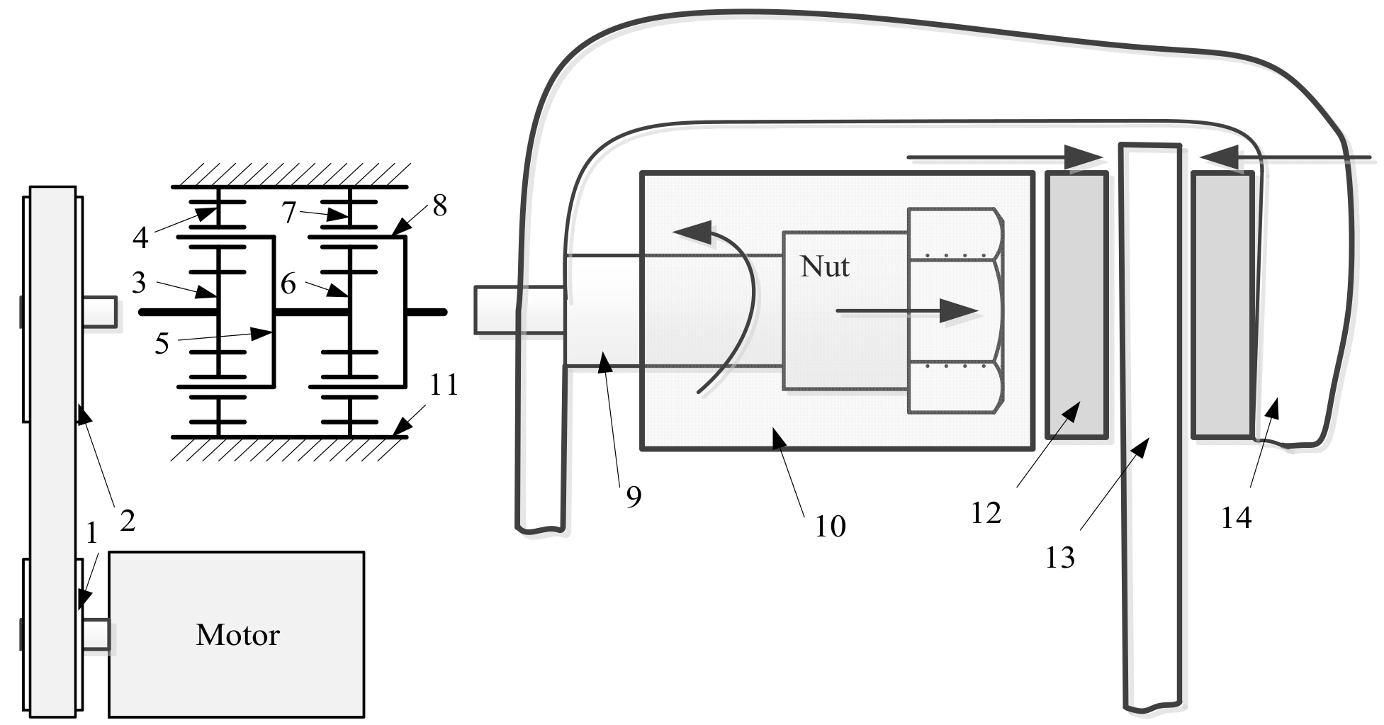
Figure 4.
Hierarchical control structure.
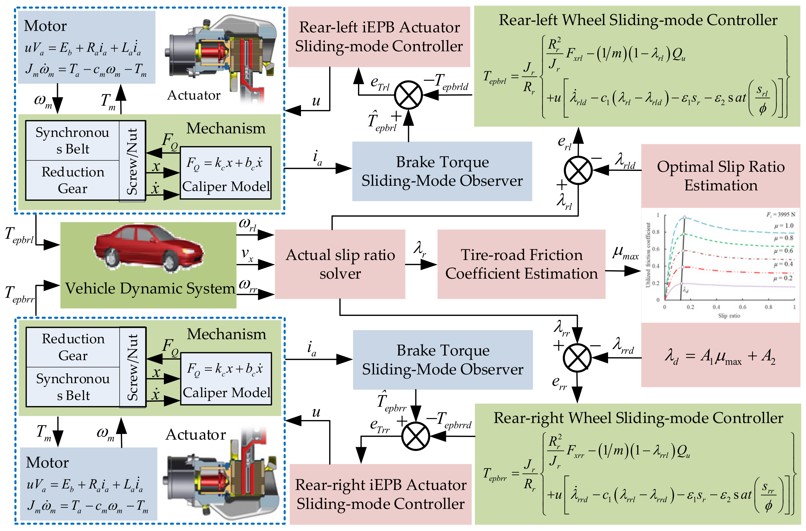
Figure 5.
HIL test bench.

Figure 6.
Experimental vehicle and devices.
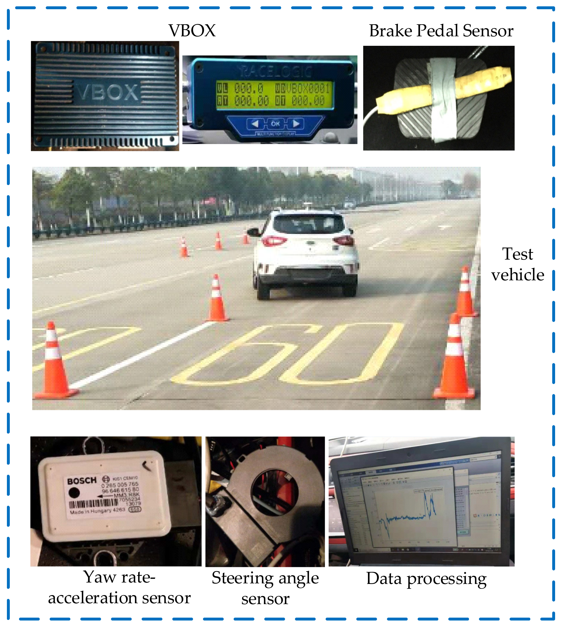
Figure 7.
Experimental and simulation results achieved under pylon course slalom maneuver: (a) lateral acceleration; (b) yaw rate.
Figure 7.
Experimental and simulation results achieved under pylon course slalom maneuver: (a) lateral acceleration; (b) yaw rate.
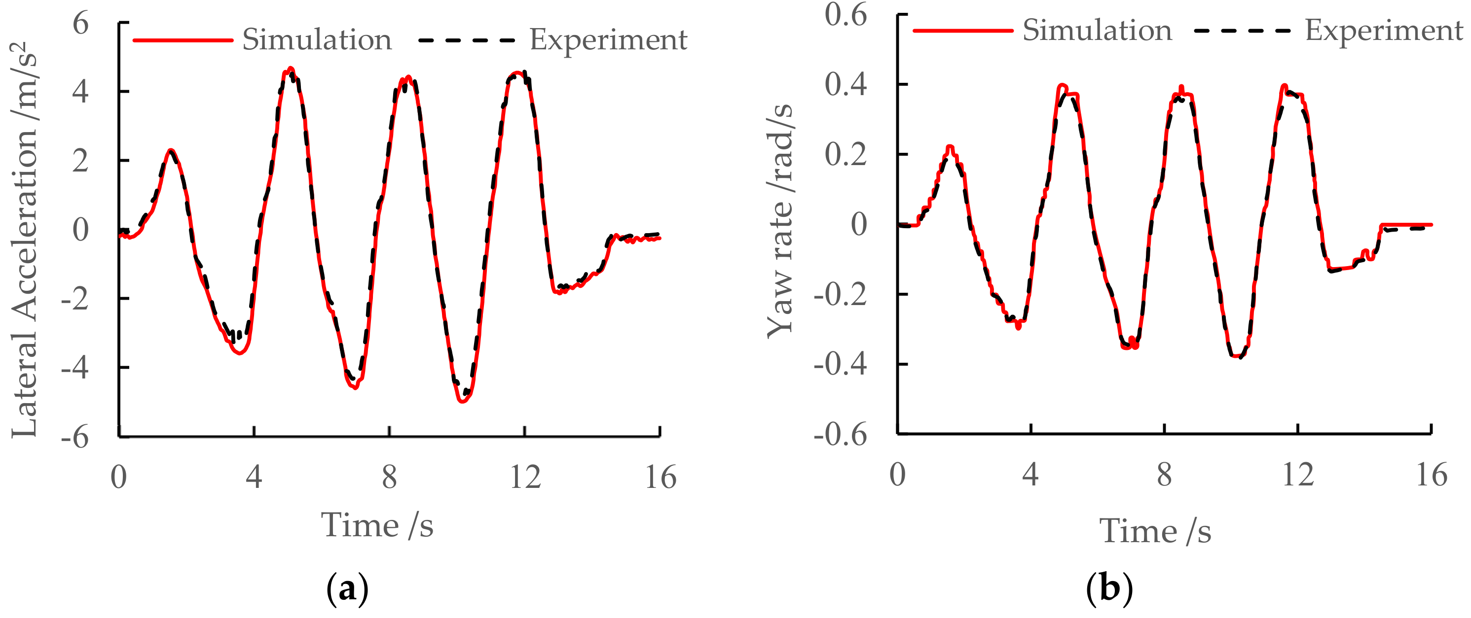
Figure 8.
The comparison between the actual and estimated load torque.
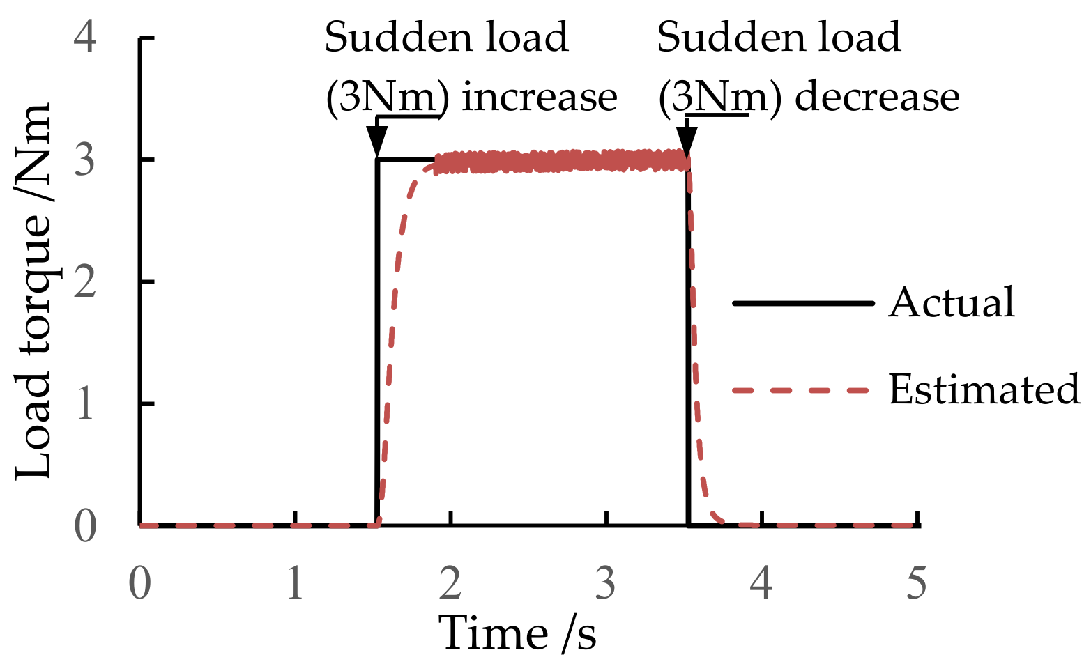
Figure 9.
HIL test results achieved under a high adhesion coefficient maneuver (vehicle longitudinal speed = 100 km/h, μ = 0.8): (1) TRFC estimation; (2) velocities of vehicle and wheels; (3) slip ratios; (4) clamping forces of RL; (5) clamping forces of RR.
Figure 9.
HIL test results achieved under a high adhesion coefficient maneuver (vehicle longitudinal speed = 100 km/h, μ = 0.8): (1) TRFC estimation; (2) velocities of vehicle and wheels; (3) slip ratios; (4) clamping forces of RL; (5) clamping forces of RR.

Figure 10.
HIL test results achieved under a low adhesion coefficient maneuver (vehicle longitudinal speed = 100 km/h, μ = 0.2): (1) TRFC estimation; (2) velocities of vehicle and wheels; (3) slip ratios; (4) clamping forces of RL; (5) clamping forces of RR.
Figure 10.
HIL test results achieved under a low adhesion coefficient maneuver (vehicle longitudinal speed = 100 km/h, μ = 0.2): (1) TRFC estimation; (2) velocities of vehicle and wheels; (3) slip ratios; (4) clamping forces of RL; (5) clamping forces of RR.

Figure 11.
HIL test results achieved under a low-to-high μ surface maneuver (vehicle longitudinal speed = 60 km/h, μ = 0.2 to 0.8): (1) TRFC estimation; (2) velocities of vehicle and wheels; (3) slip ratios; (4) clamping forces of RL; (5) clamping forces of RR.
Figure 11.
HIL test results achieved under a low-to-high μ surface maneuver (vehicle longitudinal speed = 60 km/h, μ = 0.2 to 0.8): (1) TRFC estimation; (2) velocities of vehicle and wheels; (3) slip ratios; (4) clamping forces of RL; (5) clamping forces of RR.

Figure 12.
HIL test results achieved under a μ-split surface maneuver (vehicle longitudinal speed = 50 km/h, left-side μ = 0.2, right-side μ = 0.8): (1) TRFC estimation; (2) velocities of vehicle and wheels; (3) slip ratios; (4) clamping forces of RL; (5) clamping forces of RR.
Figure 12.
HIL test results achieved under a μ-split surface maneuver (vehicle longitudinal speed = 50 km/h, left-side μ = 0.2, right-side μ = 0.8): (1) TRFC estimation; (2) velocities of vehicle and wheels; (3) slip ratios; (4) clamping forces of RL; (5) clamping forces of RR.


Table 1.
Identified parameters of the friction model.
| Symbols | Value | Symbols | Value |
|---|---|---|---|
| ap1 | −3.12 | bp1 | 148.26 |
| ap2 | 2.35 | bp2 | 60.05 |
| an1 | −3.74 | bn1 | −137.72 |
| an2 | 2.97 | bn2 | −55.79 |
| vpm (mm/s) | 6.8 | vnm (mm/s) | −6.76 |
| vpmax (mm/s) | 50 | vnmax (mm/s) | −50 |
Table 2.
Vehicle parameters.
| Parameters | Value |
|---|---|
| Vehicle mass (m) | 1855 kg |
| Tire radius (Rf, Rr) | 316 mm |
| Rotational inertia of the front/rear tire (Jf, Jr) | 1.5 kg•m2 |
| Height of the center of gravity (hg) | 530 mm |
| Distance between the front and rear axles (tw) | 2490 mm |
| Front axle to the center of gravity (a) | 1100 mm |
| Rear axle to the center of gravity (b) | 1390 mm |
| Brake disc friction coefficient (ub) | 0.35 |
| Effective brake disc radius (rp) | 105 mm |
Disclaimer/Publisher’s Note: The statements, opinions and data contained in all publications are solely those of the individual author(s) and contributor(s) and not of MDPI and/or the editor(s). MDPI and/or the editor(s) disclaim responsibility for any injury to people or property resulting from any ideas, methods, instructions or products referred to in the content. |
© 2024 by the authors. Licensee MDPI, Basel, Switzerland. This article is an open access article distributed under the terms and conditions of the Creative Commons Attribution (CC BY) license (https://creativecommons.org/licenses/by/4.0/).
Share and Cite
MDPI and ACS Style
Yong, J.; Li, L.; Wang, D.; Liu, Y. Modeling and Clamping Force Tracking Control of an Integrated Electric Parking Brake System Using Sliding-Mode-Based Observer. Actuators 2024, 13, 39. https://doi.org/10.3390/act13010039
AMA Style
Yong J, Li L, Wang D, Liu Y. Modeling and Clamping Force Tracking Control of an Integrated Electric Parking Brake System Using Sliding-Mode-Based Observer. Actuators. 2024; 13(1):39. https://doi.org/10.3390/act13010039
Chicago/Turabian StyleYong, Jiawang, Liang Li, Dongliang Wang, and Yahui Liu. 2024. "Modeling and Clamping Force Tracking Control of an Integrated Electric Parking Brake System Using Sliding-Mode-Based Observer" Actuators 13, no. 1: 39. https://doi.org/10.3390/act13010039
Note that from the first issue of 2016, this journal uses article numbers instead of page numbers. See further details here.