
Interval Type-2 Fuzzy-Model-Based Sampled-Data Control of an AUV Depth System with Input Saturation


1
Department of Control and Instrumentation Engineering, Korea Maritime and Ocean University, 727, Taejong-ro, Yeongdo-gu, Busan 49112, Republic of Korea
2
Department of Electronics and Electrical Engineering, Dankook University, 152, Jukjeon-ro, Suji-gu, Yongin-si 16890, Republic of Korea
*
Author to whom correspondence should be addressed.
Actuators 2024, 13(2), 71; https://doi.org/10.3390/act13020071
Submission received: 12 January 2024
/
Revised: 8 February 2024
/
Accepted: 9 February 2024
/
Published: 13 February 2024
(This article belongs to the Section Aircraft Actuators)
Abstract
:This paper proposes a sampled-data fuzzy controller design technique for an autonomous underwater vehicle (AUV) depth system represented by an interval type-2 (IT-2) fuzzy model, considering input saturation. In the Takagi–Sugeno (T–S) fuzzy model of an AUV depth system, surge velocity is chosen as a premise variable. To address the associated uncertainty with this variable, we employ the IT-2 fuzzy modeling technique. Also, the controller proposed in this paper utilizes time-varying gains, ensuring superior exponential stability compared with traditional fixed gain approaches. Furthermore, a membership function-dependent (MFD) criterion is employed to enhance robustness for each subsystem individually. Taking into account the mentioned aspects, the controller design condition is derived in the form of linear matrix inequalities (LMIs). Finally, the effectiveness of the proposed method is validated through simulation examples.
1. Introduction
In recent decades, the exploration of the ocean environment has been significantly enhanced through the utilization of autonomous underwater vehicles (AUVs). With ongoing advancements in AUV research, their movements have progressively become more precise, playing a crucial role in underwater exploration. To undertake various missions, AUVs require versatile capabilities, including mapping, localization, and navigation [1,2,3,4,5]. In [1], a simultaneous localization and mapping technique for AUVs was studied by employing a set membership approach. Furthermore, ref. [3] introduced a navigation strategy for AUVs based on the unscented Kalman filter. While the implementation of precise control techniques is necessary for these tasks, the design problem for AUV controllers remains challenging due to their intricate and highly nonlinear dynamics.
Researchers have shown significant interest in Takagi–Sugeno (T–S) fuzzy model-based control due to its advantages in analyzing and synthesizing nonlinear control systems [6,7,8,9]. The T–S fuzzy model represents a nonlinear system through multiple IF-THEN rules, each with a consequence part being a linear subsystem. This characteristic allows the application of conventional linear control theories to nonlinear systems. Due to these advantages, there has been some research on the T–S fuzzy model-based AUV control. In [10], researchers designed an adaptive fuzzy tracking controller using the direct adaptive fuzzy control method to alleviate the effects of actuator saturation. Additionally, in [11], the robust control problem of a perturbed T–S fuzzy-model-based lift–feedback–fin system was addressed. Previous studies, however, suffer from parameter uncertainties. In conventional studies, there exists a disparity between the actual behavior of the AUV and its T-S fuzzy model due to the assumption of unknown system parameters as constant. By extending the previous type-1 T–S fuzzy model, the interval type-2 (IT-2) fuzzy model was recently proposed. This model is constructed with upper and lower membership functions, capturing uncertainty in the system. Consequently, the IT-2 fuzzy model has been predominantly applied to systems with uncertainties [12,13,14,15,16]. Therefore, it becomes necessary to control the AUV system using an IT-2 fuzzy-model-based control approach to address uncertainties in the system dynamics effectively.
Recent advancements in computer engineering have led to the widespread implementation of control systems using digital hardware, resulting in the coexistence of continuous- and discrete-time signals within a single control system. Conventional control theories are not suitable for such systems. Therefore, researchers have studied sampled-data control theory, designed for continuous-time control systems controlled by digital hardware. Stability analysis in sampled-data control systems commonly relies on Lyapunov–Krasovskii functionals (LKFs) [17,18,19,20,21]. To mention a few notable studies, ref. [22] introduced a novel LKF with a partitioned sampling interval tailored for large sampling periods, and ref. [23] explored the memory sampled-data control method to address delayed signals between the sampler and controller. Also, in [24], the synchronization control for delayed neural networks was studied using the novel augmented Lyapunov functional, which consists of a mixed-delay-based augmented part and a time-squared two-sided looped part. In [25], a matrix-injection-based method was developed to deal with the negativity condition of the forward difference in the Lyapunov functional. However, not only are there few studies of the sampled-data control of the AUV depth system, but they also use outdated control methods.
AUVs, operating in unpredictable conditions like ocean currents and water pressure, require controllers capable of tolerating disturbances. The widely adopted control attenuates disturbance affecting T–S fuzzy model-based control systems [26,27,28,29]. Thus, there has been active research on control; for instance, in [30], performance criteria were applied to handle exogenous inputs, and ref. [31] derived static output feedback design conditions for uncertain T–S fuzzy systems under performance using switched control methods. Previous research used a fixed performance index, leading to conservativeness issues. Recently, the membership function-dependent (MFD) control, employing a distinct performance index for each rule of the T–S fuzzy model, has been explored as a less conservative alternative to the fixed approaches [32,33].
For practical applications, actuators have specified limits in force, torque, and voltage, and excessive force can potentially damage the system or degrade control performance, leading to instability. Therefore, it is crucial to consider appropriate input saturation and constraints. In this context, ref. [34] proposed less conservative sufficient conditions for nonlinear active suspension systems by addressing actuator saturation. Additionally, ref. [35] investigated active fault-tolerant control for discrete-time T-S fuzzy systems in the presence of input constraints, applying it to a three-DoF helicopter. However, to the best of the authors’ knowledge, there is a lack of studies on AUV control design considering actuator saturation.
Motivated by the aforementioned analysis, we proposed an IT-2 fuzzy sampled-data controller for a AUV depth system, accounting for uncertain parameters and actuator saturation. The main contributions of this paper are summarized as follows:
- A novel IT-2 fuzzy sampled-data controller for AUV depth systems was introduced, addressing challenges related to input saturation and uncertainty in surge velocity due to physical limitations.
- The employed controller incorporated time-varying gains, ensuring superior exponential stability in AUV depth control.
- The designed controller improved overall system robustness by applying the MFD criterion, ensuring robustness for each subsystem.
- The proposed controller design was expressed in the form of LMIs, providing a systematic and practical framework for designing an AUV depth control system.
Notation: For a positive integer a, defines an integer set . In the symmetric position of a square matrix, ∗ denotes the transposed element. For any matrix X, Sym represents . and indicate a diagonal matrix and a column vector, respectively. For a square matrix X, denotes the minimum eigenvalue of X. For a symmetric matrix X, (resp. ) means that X is positive (resp. negative) definite.
2. Problem Formulation
In this paper, we design the depth controller for the AUV described by the IT-2 fuzzy model by considering the input saturation. The IF–THEN rules for the IT-2 fuzzy model are given as follows:
where and with are the jth premise variable and its IT-2 fuzzy sets in the ith rule; , , , and are the state, saturated input, disturbance, and output vectors, respectively. In the AUV control system, , so we can say that the control input is a scalar variable. Considering the uncertainties in premise variables, the firing strength of the ith rule is described as follows:
where and represent the lower and upper grade of membership; and are the lower and upper firing strength functions satisfying . Applying the standard inference process to the above IF–THEN rules, we have
where and ; is an unknown time-varying function representing the uncertainty of the premise variables.
The bounded control input is determined by , where
where is a nonbounded control input computed by the proposed controller, and is a control input limitation determined by the physical specifications.
Next, based on the time-varying gain control concept, we propose the IT-2 fuzzy sampled-data controller with exponential time-varying gain matrices. Its IF–THEN rules are constructed as below:
for , where is the sampled-data control gain; is a given constant scalar describing the rate of change in the control gain matrices; with as the sampling time. Also, we define the sampling period as with a known . Using the same inference method as in (1), we can derive the above IF–THEN rules of the proposed controller as follows:
where
Remark 1.
Implementing the proposed controller faces two main challenges. First, solving the LMI conditions in Theorem 1 is required for the controller design. Numerical software aids in solving this condition and takes a few seconds. However, once the physical parameters of the AUV are determined, this process needs to be performed only once and is not considered a significant challenge.
Second, the controller is represented by (3), which needs to be computed at each sampling instant. Since the controller equation is similar to a typical T-S fuzzy-model-based controller, there are no particular difficulties in implementation. However, the controller in (3) contains exponentially decaying terms, which must be implemented using analog hardware. These exponentially decaying terms can be implemented by a cheap RC filter. Apart from this, there are no significantly complex or challenging issues compared with existing approaches.
Now, by using the notations and , the closed-loop IT-2 fuzzy model (1) is written as follows:
where and .
This paper aims to design the IT-2 fuzzy sampled-data controller for a AUV depth control system under the input saturation consideration. This is realized by solving the following design problem:
Problem 1.
Find the control gain matrix for the depth control system of the AUV (4) such that the following criteria are guaranteed for given scalars , , , , and h:
- (1)
- When , the equilibrium of (4) is exponentially stable with decay rate of .
- (2)
- Under the zero initial condition, the following MFD criterion is satisfiedwhere ; is given terminate time of control.
Before closing this section, we provide some lemmas that help derive the proposed controller design condition given in the next section.
Lemma 1
([36]). For positive scalar , we have the following inequality:
where X and Y are the appropriate dimensional matrices.
Lemma 2
([37]). As long as the following holds with a given scalar : , the following is always satisfied:
and hence
Lemma 3
([38]). Consider the scalars satisfying for . The inequalities hold if there exist symmetric matrices and and full rank matrices and , such that the following LMIs hold:
where , , , .
3. IT-2 Fuzzy Modeling of the AUV Depth System
In this section, we derive the IT-2 fuzzy model for the AUV depth system depicted in Figure 1. Its nonlinear dynamic equation is given as follows [39]:
where , , , and are the pitch rate, pitch angle, depth, and stern plane angle, respectively; an unknown parameter is the surge velocity; is the moment of inertia along Y axis; , , , and represent the added mass, combined term, hydrostatic, and fin lift, respectively. The actual values of all parameters are summarized in Table 1.
This paper aims to regulate the depth to the desired depth . To this end, we define the depth regulation error as . Then, the dynamics of the depth system (7) can be reformulated as follows:
We adopted a decentralized control system structure, where the surge velocity and the depth are independently regulated. Accordingly, the surge velocity, denoted as , is considered an uncertain parameter in the depth control system. Thus, we assumed that the surge velocity is an uncertain parameter varying within the range of , where and are arbitrarily selectable scalars.
Remark 2.
In prior research on fuzzy model-based control for AUV depth systems such as [39,40], the dynamic behavior was approximately linearized, or the surge velocity was treated as a constant value. In the depth control system, the actual surge velocity cannot be accurately accessed due to perturbations caused by various factors, including ocean currents. Thus, its perturbation should be captured when designing the controller. In this study, we mitigated the uncertainty in surge velocity by employing upper and lower membership functions.
Letting the premise variable be , parameters for the surge velocity be , , and the operating regions be and , we obtain the following IF-THEN rules with
where , , , , . Then, we can infer the following IT-2 fuzzy model:
where
and are the ith elements of and , respectively. The lower and upper grades of membership are determined as follows:
Setting the unknown time-varying function , are obtained
In the next section, we derive the stability and stabilization conditions for the AUV depth control system described by the IT-2 fuzzy model (8).
4. Controller Design
In this section, we derive the IT-2 fuzzy sampled-data controller design condition satisfying the design criteria given in Problem 1. First, we derive the following theorem that gives the matrix inequality condition determining whether the given control gain matrix satisfies the design criteria given in Problem 1:
Theorem 1.
For the given matrix and scalars , , , , , , , and , the design criteria given in Problem 1 are satisfied if there exist positive definite matrices , , , , , , , and ; full-rank matrices , , , , , , and ; and any matrices and such that the following matrix inequalities hold for all :
where
Proof.
Consider the following LKF:
where
where and .
First, let us define
Then, the time derivative of is obtained as below:
Next, is derived as follows:
The time derivative of is given as follows:
In (16), the integral interval of the following term can be divided as
In addition, since for , we can omit term from the above inequality. Thus, by combining and , we have
where and .
Meanwhile, letting and , the following inequalities for full-rank matrices and can be derived by [22]
Similarly, has a maximum at by differentiating it, which is bounded as follows
To apply Lemma 2, we rewrite the system (4) as follows:
Based on (23), we introduce the following null term:
The following term in (24) is obtained using Lemma 1
where is a given positive scalar. Then, applying Lemma 2, (25) can be rewritten as follows:
From (26), the following inequality is given:
where is positive scalar and .
By combining (15), (22), and (27) and considering the MFD criterion (5), we obtain the following inequality:
where
.
In addition, for , the right hand side of (28) can be reformulated as follows:
Therefore, we can say that if the following matrix inequalities hold:
Finally, by applying the Schur complement to (30) and (31), we obtain (11) and (12). In other words, if there exists a solution to the matrix inequalities of (11) and (12), then the following inequality is guaranteed:
Assuming that , we obtain
which indicates that for all t. Therefore, it is easy to prove that the following holds:
from which we can say that the first design criterion of Problem 1 is satisfied.
In addition, integrating (32) with respect to t from to under zero initial condition, we have
Since and , we can conclude that the MFD criterion is also satisfied.
On the other hand, from (3), can represented as
Remark 3.
Remark 4.
The stability condition proposed in Theorem 1 is formulated as bilinear matrix inequalities (BMIs). However, solving this condition efficiently presents challenges for contemporary numerical solvers. Additionally, the closed-loop control system involves two distinct membership functions due to uncertainties in the system’s membership function, resulting in the imperfect premise matching problem. In the subsequent theorem, we reformulate the conditions given in Theorem 1 into linear matrix inequalities (LMIs) and address the imperfect premise matching problem using the method proposed in [38].
Theorem 2.
For given scalars , , , , , , and , the system (4) holds the criteria given in Problem 1 if there exist scalars guaranteeing ; positive definite matrices , , , , , , , , , and ; full-rank matrices , , , , and ; ; and any matrices , , and such that the following LMIs satisfy for , :
where , ,
Then, the gain matrices are obtained by .
Proof.
Denote , , , , , , , , , , , , . Pre- and postmultiplying (9) and (10) by and its transpose, respectively, (35) and (36) are obtained. In addition, pre- and postmultiplying (11) and (12) by and its transpose and utilizing Lemma 3 to solve the imperfect premise matching problem, respectively, we can obtain (37)–(39). Also, by pre- and postmultiplying (13) by and its transpose, (40) is given. This completes the proof for this theorem. □
Remark 5.
When compared with existing papers, this paper considered the following improvements:
- 1
- In the conventional studies of AUV depth systems, the surge velocity was treated as a constant [39,43,44]. However, in real-world scenarios, varies due to various reasons. To address this fluctuation, this paper proposes an interval type-2 fuzzy model for the AUV’s depth system, considering as an uncertain premise variable. This approach allows the model to effectively represent the fluctuations in using its membership function.
- 2
- Typically, research on AUV depth control assumes operation in the continuous-time domain. However, due to the cost-effectiveness of digital computers, AUV control systems are generally designed as sampled-data systems, where the plant and controller operate in different time domains. Although there are existing studies on sampled-data control for the AUV depth system, they rely on traditional sampled-data control techniques [45,46]. Motivated by this observation, this paper introduces a novel approach to control the AUV depth system by combining a recently developed sampled-data control method with an IT-2 fuzzy model for the AUV depth control system.
- 3
- Previous studies on AUV depth control systems have not extensively addressed real-world challenges like fault estimation, tolerance control, and control input saturation. Control input saturation, in particular, presents a significant limitation for AUV depth control systems. This is due to the physical constraints on the control input, which is typically related to the angle of a fin lift and is limited in its operational range. By addressing the input saturation problem, this paper proposes a more practical controller design strategy for AUV depth control systems than the previous studies.
5. Simulation Validation
In this section, we illustrate the design process of an IT-2 fuzzy sampled-data controller for an AUV depth system, considering input saturation. Furthermore, we evaluate and analyze the performance of the designed controller through simulation examples.
The parameter values for solving the LMIs presented in Theorem 2 (35)–(40) are chosen as follows: decay rate and , sampling period , input saturation , bounds on the membership functions , and remaining constants , , , , , and . From the selection of the parameters, we can see that the maximum allowable sampling period is , which means that the controller operates at . From the solution, we obtain the following control gains:
Now, we analyze the control performance of the designed control system. In the simulation, we demonstrate the regulation of the depth of the AUV to . For this purpose, we initialize the system with , indicating that the pitch, pitch rate, and depth are all zero at the start of control. In addition, to validate the disturbance attenuation performance, we arbitrarily chose the disturbance as .
The results of the AUV depth control are illustrated in Figure 2, Figure 3, Figure 4 and Figure 5. In Figure 2, the time responses of and are presented. The AUV regulates its depth by adjusting its pitch angle. As depicted in Figure 2, from 0 s to 2 s, the AUV’s pitch angle rotates to adjust its depth. Once the depth is regulated, the pitch rate is perturbed to robustly maintain the depth even in the presence of disturbances.
In Figure 3, the time responses of the depth controlled by both the proposed method and the method from [47] are presented. The approach in [47] does not account for input saturation. However, since the AUV in this simulation has limitations on the fin-lift angle, both time responses are obtained equally considering input saturation. The control input trajectories are displayed in Figure 4. As shown in Figure 4, the control input is saturated, even though the controller designed by [47] does not compensate for it. Consequently, as observed in Figure 3, the proposed controller exhibits less perturbation in the AUV’s depth, attributed to the consideration of input saturation. Additionally, as , the depth of the AUV given by converges to , which meets the objective of this simulation.
Next, the trajectory of the MFD performance index and fixed performance index are shown in Figure 5. The MFD performance index is obtained by
Therefore, we observe that it changes in , and it varies within the ranges of . As depicted in the figure, the proposed MFD index exhibits better disturbance attenuation performance compared with the fixed index when .
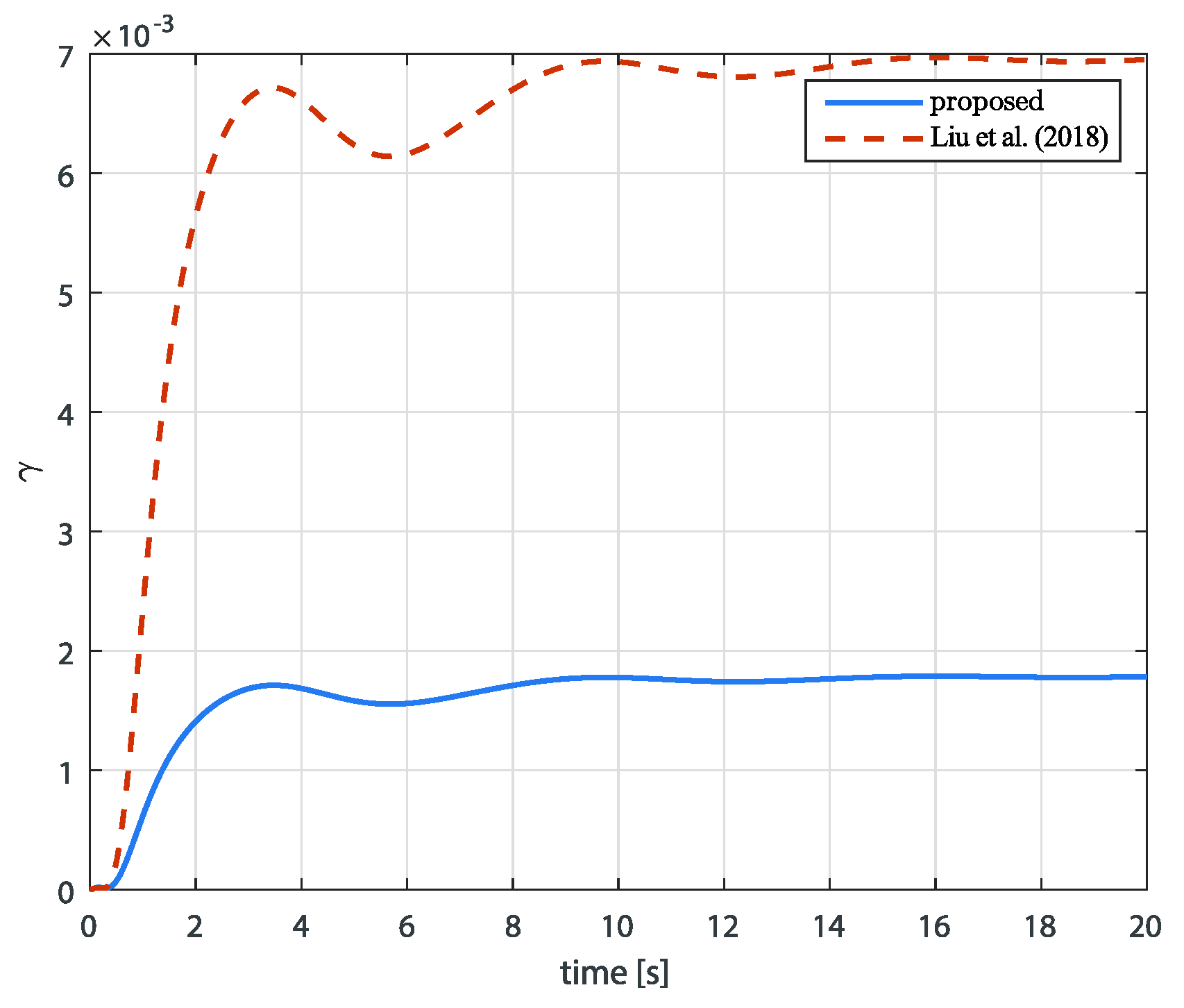
Next, we show the comparison of the disturbance attenuation performance of the proposed method with [47]. As in the second objective in Problem 2, we set the initial condition as , indicating that the pitch, pitch rate, and depth are all zero at the start of control. In the comparison, the disturbance was set as , and the control gain is the same as in the previous setting. In Figure 6, the results of the norm ratio of to are depicted. The results demonstrate that the proposed method provides better disturbance attenuation performance than [47]. This is due to the MFD criterion considering the disturbance attenuation performance of each subsystem.
Summarizing the aforementioned analysis, the simulation results indicate that the proposed method outperforms the previous study in disturbance attenuation performance, even in the presence of the actuator limitation. Additionally, the MFD approach demonstrates superior disturbance attenuation performance compared with the fixed -based method.
6. Conclusions
This paper presented a technique for designing a sampled-data fuzzy controller for an AUV depth system represented by an IT-2 fuzzy model, taking into account input saturation. The surge velocity was chosen as the premise variable to capture the perturbations in the surge velocity. As the premise variable is uncertain, the IT-2 fuzzy modeling technique was employed in this paper. The controller designed in this paper employed time-varying gains, ensuring superior exponential stability compared with conventional fixed gain approaches. Additionally, an MDF criterion was used to enhance robustness for each subsystem individually. Combining the proposed techniques, the controller design conditions were formulated as LMIs from the LKF. Finally, by simulation, we validated that the proposed method achieves better robustness compared with a previous study.
When we conducted a simulation using the method [38] to solve the imperfect premise problem, there was a problem that the dimension of LMIs was too large and the gain calculation took too long. Thus, in future work, we will study a simple and effective method to address the imperfect premise problem. Also, we will study a method of relaxing the conservativeness by constructing novel LKFs using a variety of methods, such as in [24,25].
Author Contributions
Conceptualization, J.H.A.; Validation, J.H.A.; Writing—original draft, J.H.A.; Writing—review & editing, H.S.K.; Supervision, H.S.K. All authors have read and agreed to the published version of the manuscript.
Funding
This research received no external funding.
Data Availability Statement
The data presented in this study are available in article here.
Conflicts of Interest
The authors declare no conflicts of interest.
References
- Jaulin, L. A nonlinear set membership approach for the localization and map building of underwater robots. IEEE Trans. Robot. 2009, 25, 88–98. [Google Scholar] [CrossRef]
- Paull, L.; Saeedi, S.; Seto, M.; Li, H. AUV navigation and localization: A review. IEEE J. Ocean. Eng. 2014, 39, 131–149. [Google Scholar] [CrossRef]
- Allotta, B.; Caiti, A.; Costanzi, R.; Fanelli, F.; Fenucci, D.; Meli, E.; Ridolfi, A. A new AUV navigation system exploiting unscented Kalman filter. Ocean Eng. 2016, 113, 121–132. [Google Scholar] [CrossRef]
- Ma, T.; Li, Y.; Wang, R.; Cong, Z.; Gong, Y. AUV robust bathymetric simultaneous location and mapping. Ocean Eng. 2018, 166, 336–349. [Google Scholar] [CrossRef]
- Kapoutsis, A.C.; Chatzichristofis, S.A.; Doitsidis, L.; de Sousa, J.B.; Braga, J.; Kosmatopoulos, E.B. Real-time adaptive multi-robot exploration with application to underwater map construction. Auton. Robot. 2016, 40, 987–1015. [Google Scholar] [CrossRef]
- Fang, C.; Liu, Y.; Kau, S.; Hong, L.; Lee, C. A new LMI-based approach to relaxed quadratic stabilization of T–S fuzzy control systems. IEEE Trans. Fuzzy Syst. 2006, 14, 386–397. [Google Scholar] [CrossRef]
- Mrazgua, J.; Chaibi, R.; Tissir, E.H.; Ouahi, M. Static output feedback stabilization of T–S fuzzy active suspension system. J. Terramechanics 2021, 97, 19–27. [Google Scholar] [CrossRef]
- Mu, Y.; Zhang, H.; Xi, R.; Gao, Z. State and fault estimations for discrete-time T–S fuzzy systems with sensor and actuator faults. IEEE Trans. Circuits Syst. II Express Brief 2021, 68, 3326–3330. [Google Scholar] [CrossRef]
- Vu, V.; Wang, W. Polynomial controller synthesis for uncertain large-scale polynomial T–S fuzzy systems. IEEE Trans. Cybern. 2021, 51, 1929–1942. [Google Scholar] [CrossRef]
- Yu, C.; Zhang, Q.; Xu, G. Adaptive fuzzy trajectory tracking control of an under-actuated autonomous underwater vehicle subject to actuator saturation. Int. J. Fuzzy Syst. 2018, 20, 269–279. [Google Scholar] [CrossRef]
- Chang, C.; Chang, W. Robust fuzzy control with transient and steady-state performance constraints for ship fin stabilizing sys-tems. Int. J. Fuzzy Syst. 2018, 21, 518–531. [Google Scholar] [CrossRef]
- Li, H.; Wang, J.; Lam, H.K.; Zhou, Q.; Du, H. Adaptive sliding mode control for interval type-2 fuzzy systems. IEEE Trans. Syst. Man, Cybern. Syst. 2016, 46, 1654–1663. [Google Scholar] [CrossRef]
- Zhang, Z.; Zhou, Q.; Wu, C.; Li, H. Dissipativity-based reliable interval type-2 fuzzy filter design for uncertain nonlinear systems. Int. J. Fuzzy Syst. 2018, 20, 390–402. [Google Scholar] [CrossRef]
- Xiao, B.; Lam, K.K.; Song, G.; Li, H. Output-feedback tracking control for interval type-2 polynomial fuzzy-model-based control systems. Neurocomputing 2017, 242, 83–95. [Google Scholar] [CrossRef]
- Song, W.; Tong, S. Fuzzy decentralized output feedback event-triggered control for interval type-2 fuzzy systems with satu-rated inputs. Inf. Sci. 2021, 575, 639–653. [Google Scholar] [CrossRef]
- Rong, N.; Wang, Z. Event-based impulsive control of IT2 T–S fuzzy interconnected system under deception attacks. IEEE Trans. Fuzzy Syst. 2021, 29, 1615–1628. [Google Scholar] [CrossRef]
- Zeng, H.B.; Teo, K.L.; He, Y.; Wang, W. Sampled-data stabilization of chaotic systems based on a T–S fuzzy model. Inf. Sci. 2019, 483, 262–272. [Google Scholar] [CrossRef]
- Hua, C.; Wu, S.; Guan, X. Stabilization of T–S fuzzy system with time delay under sampled-data control using a new looped-functional. IEEE Trans. Fuzzy Syst. 2020, 28, 400–407. [Google Scholar] [CrossRef]
- Cai, X.; Wang, J.; Zhong, S.; Shi, K.; Tang, Y. Fuzzy quantized sampled-data control for extended dissipative analysis of T–S fuzzy system and its ap-plication to WPGSs. J. Frankl. Inst. 2021, 358, 1350–1375. [Google Scholar] [CrossRef]
- Kim, H.S.; Lee, K.; Joo, Y.H. Decentralized sampled-data fuzzy controller design for a VTOL UAV. J. Frankl. Inst. 2021, 358, 1888–1914. [Google Scholar] [CrossRef]
- Zhai, Z.; Yan, H.; Chen, S.; Zhan, X.; Zeng, H. Further results on dissipativity analysis for T–S fuzzy systems based on sampled-data control. IEEE Trans. Fuzzy Syst. 2023, 31, 660–668. [Google Scholar] [CrossRef]
- TLee, H.; Park, J.H. New methods of fuzzy sampled-data control for stabilization of chaotic systems. IEEE Trans. Syst. Man, Cybern. Syst. 2018, 48, 2026–2034. [Google Scholar]
- Ge, C.; Shi, Y.; Park, J.H.; Hua, C. Robust H∞ stabilization for T-S fuzzy systems with time-varying delays and memory sam-pled-data control. Appl. Math. Comput. 2019, 346, 500–512. [Google Scholar]
- Zhang, Y.; He, Y.; Long, F.; Zhang, C. Mixed-delay-based augmented functional for sampled-data synchronization of delayed neural networks with communication delay. IEEE Trans. Neural Netw. Learn. Syst. 2022, 35, 1847–1856. [Google Scholar] [CrossRef] [PubMed]
- Zhang, C.; Xie, K.; He, Y.; She, J.; Wu, M. Matrix-injection-based transformation method for discrete-time systems with time-varying delay. Sci. China Inf. Sci. 2023, 66, 159201. [Google Scholar] [CrossRef]
- Shi, J.; Zhang, Q. Dynamic sliding-mode control for T–S fuzzy singular time-delay systems with H∞ performance. IEEE Access 2019, 7, 115388–115399. [Google Scholar] [CrossRef]
- Xie, W.; Wang, T.; Zhang, J.; Wang, Y. H∞ reduced-order observer-based controller synthesis approach for T–S fuzzy systems. J. Frankl. Inst. 2019, 356, 6388–6400. [Google Scholar] [CrossRef]
- Han, T.J.; Kim, H.S. Disturbance observer-based nonfragile fuzzy tracking control of a spacecraft. Adv. Space Res. 2023, 71, 3600–3612. [Google Scholar] [CrossRef]
- Yan, S.; Gu, Z.; Ding, L.; Park, J.H.; Xie, X. Weighted memory H∞ stabilization of time-varying delayed Takagi–Sugeno fuzzy systems. IEEE Trans. Fuzzy Syst. 2023, 32, 337–342. [Google Scholar] [CrossRef]
- Klug, M.; Catelan, E.B.; Coutinho, D. A T-S fuzzy approach to the local stabilization of nonlinear discrete-time systems subject to ener-gy-bounded disturbances. J. Control Autom. Electr. Syst. 2015, 26, 191–200. [Google Scholar] [CrossRef]
- Elias, L.J.; Faria, F.A.; Araujo, R.; Magossi, R.F.Q.; Oliveira, V.A. Robust static output feedback H∞ control for uncertain Takagi–Sugeno fuzzy systems. IEEE Trans. Fuzzy Syst. 2022, 30, 4434–4446. [Google Scholar] [CrossRef]
- Dong, J.; Hou, Q.; Ren, M. Control synthesis for discrete-time T–S fuzzy systems based on membership function-dependent H∞ performance. IEEE Trans. Fuzzy Syst. 2019, 28, 3360–3366. [Google Scholar] [CrossRef]
- Kuppusamy, S.; Joo, Y.H. Stabilization criteria for T–S fuzzy systems with multiplicative sampled-data control gain uncertainties. IEEE Trans. Fuzzy Syst. 2022, 30, 1082–4092. [Google Scholar] [CrossRef]
- Xie, Z.; Wang, D.; Wong, P.K.; Li, W.; Zhao, J. Dynamic-output-feedback based interval type-2 fuzzy control for nonlinear active suspension systems with actuator saturation and delay. Inf. Sci. 2022, 607, 1174–1194. [Google Scholar] [CrossRef]
- Zare, I.; Setoodeh, P.; Asemani, M.H. Fault-tolerant tracking control of discrete-time T-S fuzzy systems with input constraint. IEEE Trans. Fuzzy Syst. 2022, 30, 1914–1928. [Google Scholar] [CrossRef]
- Wu, C.; Chen, B.; Zhang, W. Multipleobjective H2/H∞ control design of the nonlinear mean-field stochastic jump-diffusion system via fuzzy approach. IEEE Trans. Fuzzy Syst. 2019, 27, 686–700. [Google Scholar] [CrossRef]
- Du, H.; Zhang, N.; Ji, J.C.; Gao, W. Robust fuzzy control of an active magnetic bearing subject to voltage saturation. IEEE Trans. Control. Syst. Technol. 2010, 18, 164–169. [Google Scholar] [CrossRef]
- Arino, C.; Sala, A. Extensions to stability analysis of fuzzy control systems subject to uncertain grades of membership. IEEE Trans. Syst. Man Cybern.-Part B Cybern. 2008, 38, 558–563. [Google Scholar] [CrossRef]
- Prestero, T. Verification of a Six-Degree of Freedom Simulation Model for the REMUS Autonomous Underwater Vehicle. Master’s Thesis, Department of Ocean Engineering and Mechanical Engineering, Massachusetts Institute of Technology, Cambridge, MA, USA, 2001. [Google Scholar]
- Lei, M. Nonlinear diving stability and control for an AUV via singular perturbation. Ocean Eng. 2020, 197, 106824. [Google Scholar] [CrossRef]
- Cao, Y.Y.; Lin, Z. Robust stability analysis and fuzzy scheduling control for nonlinear systems subject to actuator saturation. IEEE Trans. Fuzzy Syst. 2003, 11, 57–67. [Google Scholar]
- Wang, X.; Park, J.H.; Yang, H.; Zhao, G.; Zhong, S. An improved fuzzy sampled-data control to stabilization of T-S fuzzy systems with state delays. IEEE Trans. Cybern. 2020, 50, 3125–3135. [Google Scholar] [CrossRef]
- Li, J.; Lee, P. Design of an adaptive nonlinear controller for depth control of an autonomous underwater vehicle. Ocean Eng. 2005, 32, 2165–2181. [Google Scholar] [CrossRef]
- Shen, Y.; Shao, K.; Ren, W.; Li, Y. Diving control of autonomous underwater vehicle based on improved active disturbance rejection control approach. Neurocomputing 2016, 173, 1377–1385. [Google Scholar] [CrossRef]
- Kim, D.W.; Lee, H.J.; Kim, M.H.; Lee, S.; Kim, T. Robust sampled-data fuzzy control of nonlinear systems with parametric uncertainties: Its application to depth control of autonomous underwater vehicles. Int. J. Control Autom. Syst. 2012, 10, 1164–1172. [Google Scholar] [CrossRef]
- Ma, C.; Qiao, H.; Kang, E. Mixed H∞ and passive depth control for autonomous underwater vehicles with fuzzy memorized sampled-data controller. Int. J. Fuzzy Syst. 2017, 20, 621–629. [Google Scholar] [CrossRef]
- Liu, Y.; Park, J.H.; Guo, B.; Shu, Y. Further results on stabilization of chaotic systems based on fuzzy memory sampled-data control. IEEE Trans. Fuzzy Syst. 2018, 26, 1040–1045. [Google Scholar] [CrossRef]
Figure 1.
The AUV body—fixed and inertial coordinate systems.
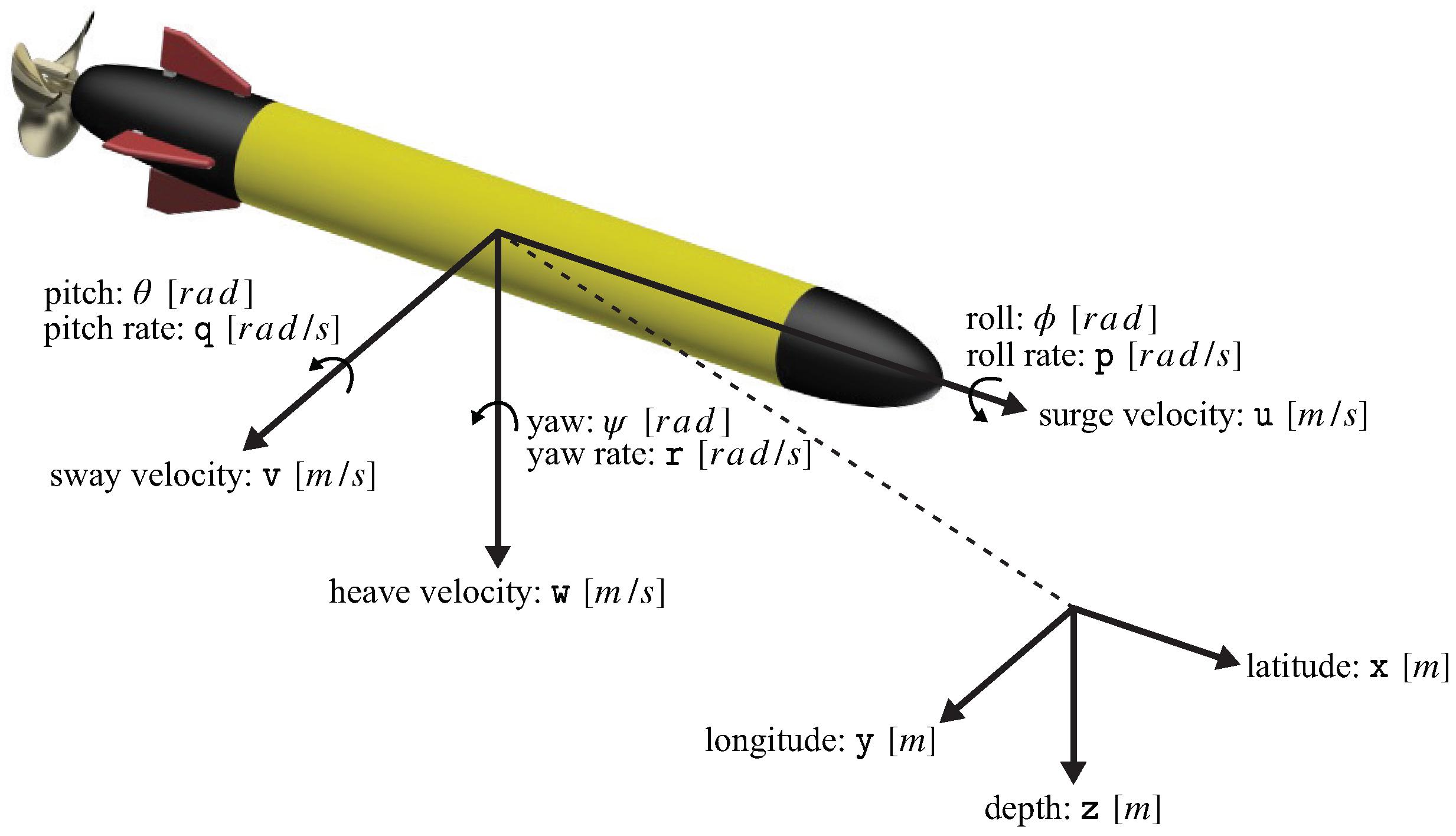
Figure 2.
The state trajectories and of the control system designed by Theorem 2.
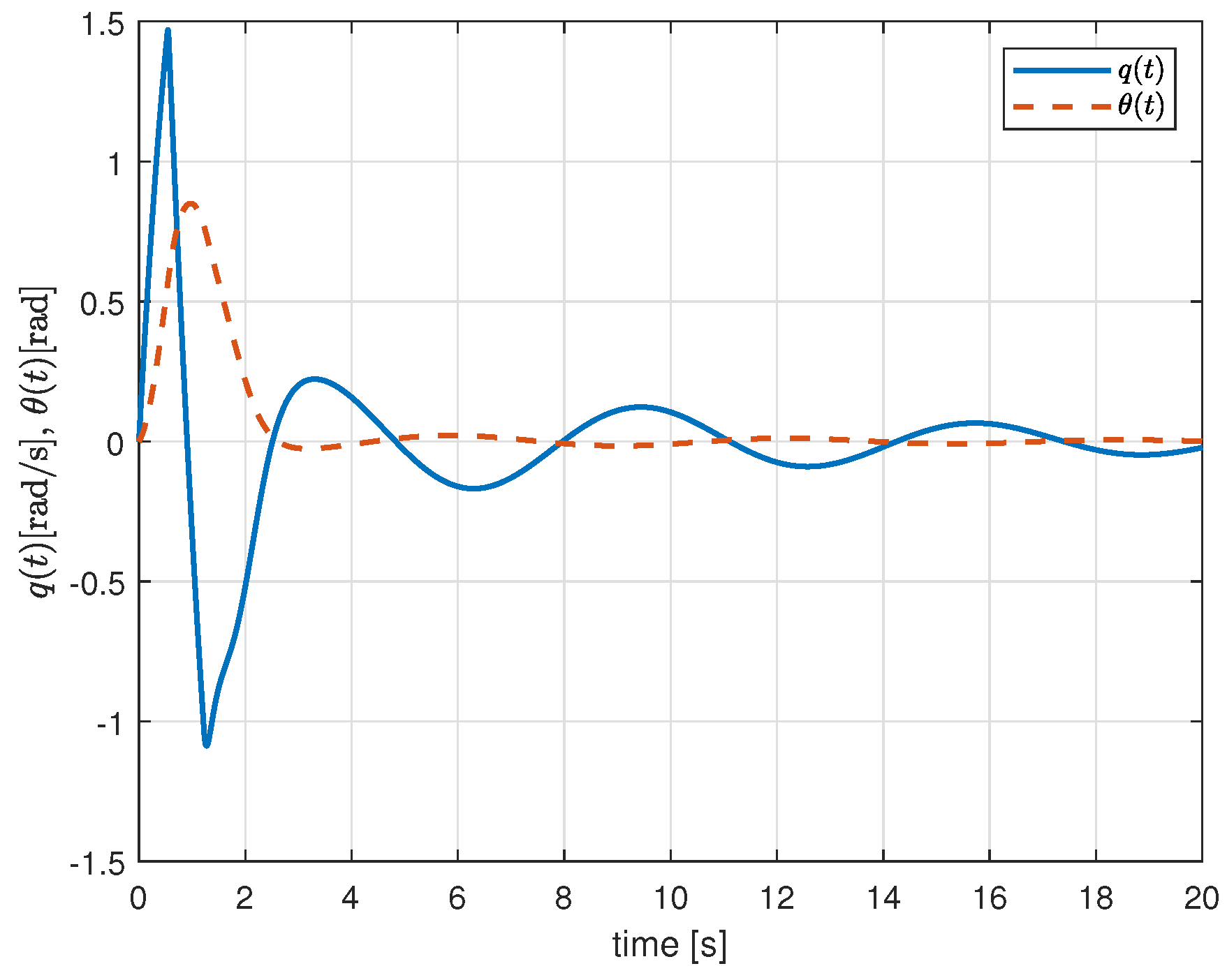
Figure 3.
The state trajectories of the depth error of the control system designed by Theorem 2 and Liu et al. (2018) [47].
Figure 3.
The state trajectories of the depth error of the control system designed by Theorem 2 and Liu et al. (2018) [47].
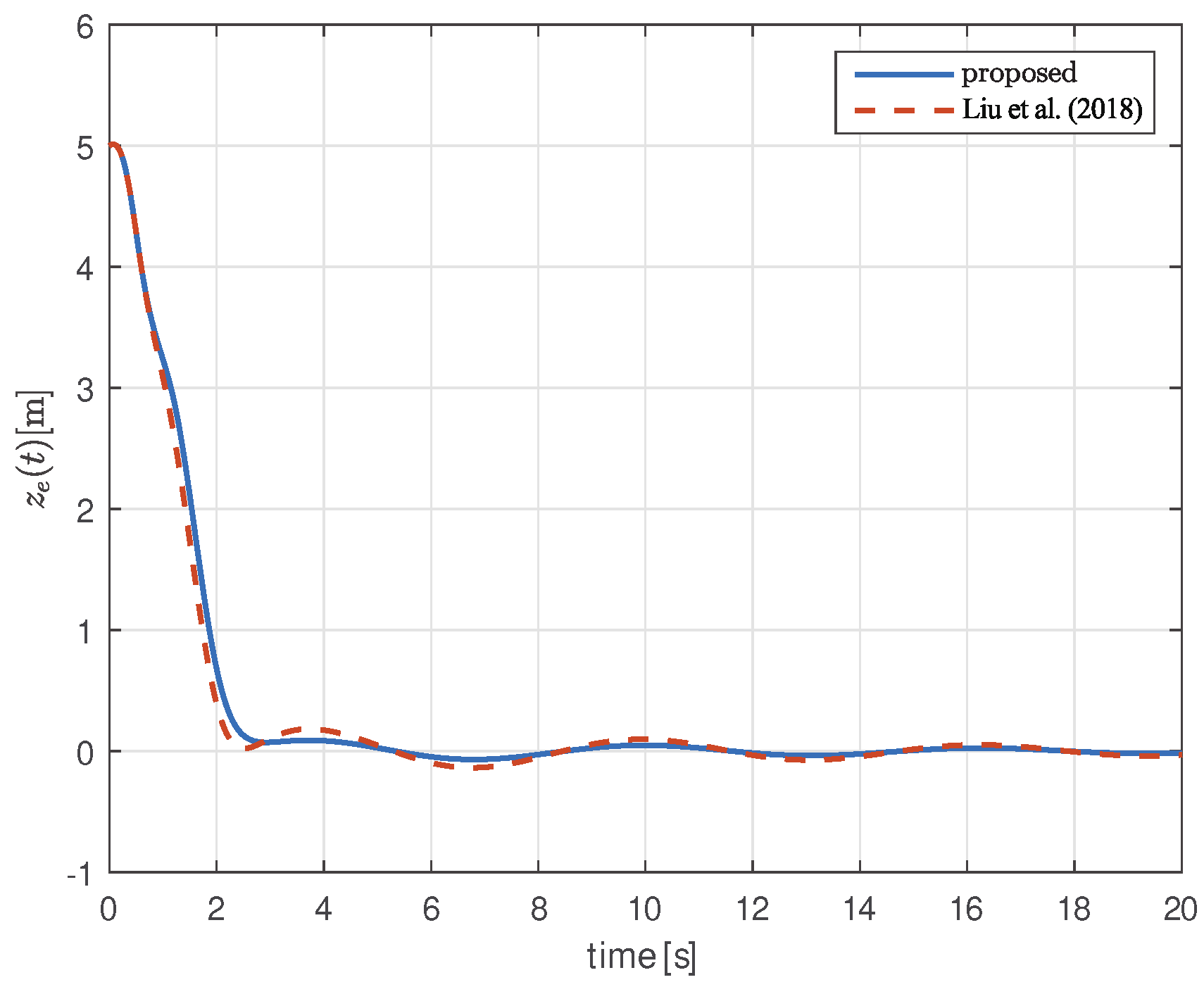
Figure 4.
The time response of the by Theorem 2 and Liu et al. (2018) [47].
Figure 4.
The time response of the by Theorem 2 and Liu et al. (2018) [47].
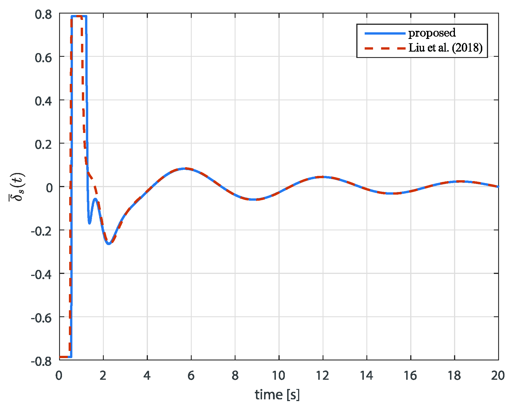
Figure 5.
The trajectory of the MFD and fixed .

Figure 6.
The trajectory of performance index by Theorem 2 and Liu et al. (2018) [47].
Figure 6.
The trajectory of performance index by Theorem 2 and Liu et al. (2018) [47].

Table 1.
The parameters of the AUV.
| Parameter | Value | Parameter | Value |
|---|---|---|---|
Disclaimer/Publisher’s Note: The statements, opinions and data contained in all publications are solely those of the individual author(s) and contributor(s) and not of MDPI and/or the editor(s). MDPI and/or the editor(s) disclaim responsibility for any injury to people or property resulting from any ideas, methods, instructions or products referred to in the content. |
© 2024 by the authors. Licensee MDPI, Basel, Switzerland. This article is an open access article distributed under the terms and conditions of the Creative Commons Attribution (CC BY) license (https://creativecommons.org/licenses/by/4.0/).
Share and Cite
MDPI and ACS Style
An, J.H.; Kim, H.S. Interval Type-2 Fuzzy-Model-Based Sampled-Data Control of an AUV Depth System with Input Saturation. Actuators 2024, 13, 71. https://doi.org/10.3390/act13020071
AMA Style
An JH, Kim HS. Interval Type-2 Fuzzy-Model-Based Sampled-Data Control of an AUV Depth System with Input Saturation. Actuators. 2024; 13(2):71. https://doi.org/10.3390/act13020071
Chicago/Turabian StyleAn, Ji Ho, and Han Sol Kim. 2024. "Interval Type-2 Fuzzy-Model-Based Sampled-Data Control of an AUV Depth System with Input Saturation" Actuators 13, no. 2: 71. https://doi.org/10.3390/act13020071
Note that from the first issue of 2016, this journal uses article numbers instead of page numbers. See further details here.