State Space System Identification of 3-Degree-of-Freedom (DOF) Piezo-Actuator-Driven Stages with Unknown Configuration

Abstract

Due to their fast response, high accuracy and non-friction force, piezo-actuators have been widely employed in multiple degree-of-freedom (DOF) stages for various nano-positioning applications. The use of flexible hinges in these piezo-actuator-driven stages allows the elimination of the influence of friction and backlash clearance, as observed in other configurations; meanwhile it also causes more complicated stage performance in terms of dynamics and the cross-coupling effect between different axes. Based on the system identification technique, this paper presents the development of a model for the 3-DOF piezo-actuator-driven stages with unknown configuration, with its parameters estimated from the Hankel matrix by means of the maximum a posteriori (MAP) online estimation. Experiments were carried out on a commercially-available piezo-actuator-driven stage to verify the effectiveness of the developed model, as compared to other methods. The results show that the developed model is able to predict the stage performance with improved accuracy, while the model parameters can be well updated online by using the MAP estimation. These capabilities allow investigation of the complicated stage performance and also provide a starting point from which the mode-based control scheme can be established for improved performance.

1. Introduction

Piezo-actuator-driven stages have the advantages of fast response, high precision and generation of large forces. As such, they have been widely applied in semiconductors, biomedical science, production manufacturing and other devices that require nano-positioning and manipulation [1,2,3,4,5]. With the ingenious design of flexible hinges, friction and backlash clearance can be eliminated, leading to improved performance. Meanwhile, the use of flexible hinges also caused a more complicated stage. Modeling and control for one degree-of-freedom (DOF) piezo-actuator-driven stages have drawn considerable attention in the literature [6,7,8,9,10]. Due to the cross-coupling effect between different axes, the methods developed for 1-DOF piezo-actuator-driven stages may not be readily extended to multiple-axis ones [11], the research of which is still in its early stage. In [12], a three-input-three-output state space model was developed for a 3-DOF micro-stage, along with the method for parameter identification; and by experiments, it was shown that the developed model was able to predict the performance of the micro-stage with acceptable accuracy. An auto-regressive exogenous (ARX) model was developed in [13] to describe the dynamic performance of a biaxial piezo-stage, and the model was then integrated in a feedforward compensator for precision tracking control with experimental verification. However, the cross-coupling between the two axes, which might have a negative effect on the performance of the controller, was not considered in the ARX model. In [14], a fourth order linear transfer function was identified for a piezoelectric stage, where the cross-coupling effect was neglected. On this basis, a chirp signal was applied to each of the axes independently, and with the measurement outputs, the parameters in each transfer function were estimated by using the system identification technique. In [15], the dynamic equations were combined with the Bouc-Wen model for each piezoelectric actuator to describe the performance of a plane-type 3-DOF precision positioning table or stage. The parameters of the model were optimized based on the real-coded genetic algorithm (RGA) method. From the numerical simulations and experimental results, the 3-DOF cross-coupling effect was reduced by the proposed control method, and good contour tracking performance was obtained, due to successful identification of the dynamic models.

A straightforward modeling method for multi-DOF piezo-actuator-driven stages can be based on the internal configuration by means of physics laws, as mentioned above. However, such details with regard to the internal structure are often not provided by the manufactures. Therefore, system identification for multi-DOF piezo-actuator-driven stages with unknown configuration is always required for the model development. In [16] and [17], modeling of a commercially available 3-DOF piezo-actuator-driven stage was formulated as a single-input-single-output nonlinear regression problem, with the cross-coupling effect ignored. By employing the online least squares support vector machine and relevance vector machine, the model parameters were updated, once the subsequent measurement became available. The developed model was applied to the inverse-model-based feedforward control scheme combined with proportional-integral-derivative (PID) regulator, and the performance of the piezo-actuator-driven stage being controlled was improved. An alternative method to improve the performance of multi-DOF piezo-actuator-driven stage is the use of a robust linear controller, such as the sliding mode controller [18], in which the nonlinear effects are regarded as disturbance and then rejected by the robust controller. As such, a linear state space model for the multi-DOF piezo-actuator-driven stage is always desired. To meet this need, in this paper, we report the model development based on the black box system identification of for 3-DOF piezo-actuator-driven stages with unknown configuration. Specifically, a linear discrete state space model, x(k+1) = Ax(k) + Bu(k) and y(k) = Cx(k) + Du(k) (A, B, C and D are system matrices), is adopted and applied to describe the dynamics of the piezo-actuator-driven stage.

To identify the parameters of the state space model, methods have been reported in the literature [19,20,21,22,23,24,25]. In [22], a modified frequency domain subspace identification algorithm was developed based on the previous work. The power spectrum estimates was strongly consistent when the measurements were corrupted by bounded random noise. In [23], the numerical algorithms for the subspace state space system identification (N4SID) method was combined with the multivariable output-error state space (MOESP) method for improved performance. The state space model was obtained in [24] by identifying the Markov parameters (a kind of matrix impulse response) that were indirectly calculated from an identified auto-regressive model or transfer function. In [25], the system matrices in the state space model were derived through singular value decomposition (SVD) of the Hankel matrix, which was directly identified from a Hankel-Toeplitz model using the least squares method. The parameters are time-invariant, and thus, the model cannot be applied if the performance of piezo-actuator-driven stage changes with the environmental condition, such as the temperature.

To develop a state space model with updating parameters, the SVD of the Hankel matrix is strategically combined with maximum a posteriori (MAP) online estimation in this study. The parameters can be updated as new observations become available. Furthermore, MAP estimation utilizes prior information regarding the parameters and the measurement errors. Inclusion of posteriori parameter information can have the beneficial effect of reducing the variances of parameter estimators. To verify the effectiveness of the state space model identified by using the MAP online estimation, experiments were carried out on a commercially available piezo-actuator-driven stage. The estimation errors obtained from the Hankel matrix using online estimation were compared to those reported in [25], for the illustration of the proposed method effectiveness.

2. System Identification for a 3-DOF Piezo-Actuator-Driven Stage with Unknown Configuration

In this section, it is assumed that the configuration or the internal structure of 3-DOF piezo-actuator-driven stages is unknown. Also, it is assumed that the stage is regarded as a linear multiple-input and multiple-output (MIMO) system by ignoring the nonlinearity, which is reasonable, as illustrated in the experiments presented later in this paper. To represent the linear dynamics and cross-coupling effect of the stage, the simplified Hankel-Toeplitz model is adopted and employed in the present study, in which the Hankel matrix is to be identified by implementing the MAP online estimation method.

2.1. Simplified Hankel-Toeplitz Model

For a linear MIMO system, the discrete state space representation is given by:

(1)

where , , and are system matrices, is the state, is the input, is the output, and represent the ignored nonlinearity and uncertainties of the piezo-actuator-driven stage and m and q are the number of inputs and outputs, respectively. By iteration, one has:

(2)

for any , where u_p and y_p are defined as column vectors of the input and output data going p steps towards the future,

(3)

v_p and w_p are defined as column vectors of the noises and disturbance going p steps towards the future, B_p is the controllability matrix, C_p is the observability matrix, D_p is the Toeplitz matrix for the system Markov parameters and

(4)

If , there exists an interaction matrix M such that:

(5)

Substituting Equation (5) into Equation (2) yields:

(6)

Combining Equations (2) and (6) leads to the following equation, which is the so-called simplified Hankel-Toeplitz model:

(7)

where

Using the following denotations:

(8)

one has Equation (7) rewritten as:

(9)

where represents the combined model noises and can be regarded as the model estimation error.

Define:

(10)

the square matrix, H₀, can be estimated without knowing M.

Once H₀ is identified, an adjacent can be calculated by using Equation (5) such that:

(11)

Similarly,

(12)

Using as building blocks, a Hankel matrix of any size can be constructed. For example:

(13)

2.2. Reconstruction of the System Matrices

The Hankel matrix is arranged with Markov parameters of increasing order going from left to right. Let the Hankel matrices be:

(14)

where . Comparing Equation (14) with Equations (4), (12) and (13); and can then be extracted from H by rearrangement of its elements. The state space matrices are reconstructed from the Hankel matrix by employing the following Lemma 1.

Lemma 1: An s-th order state space model can be reconstructed as:

(15)

where B is the first m columns of , C is the first q rows of and . The matrix U_s and V_s are made up of s left and right singular vectors of , and the diagonal matrix, , is made up of s corresponding singular values of [24].

2.3. MAP Online Estimation

Equation (9) can be rewritten as, by ignoring :

(16)

where

By using the least squares method, θ is identified to be a time-invariant matrix, which might not be able to accurately describe the environment-dependent performance of the piezo-actuator drive stage. In order to apply the state space model in the control of piezo-actuator-driven stage, the model parameters should be updated as new observation data is available. Therefore, MAP online estimation was employed to identify the parameter matrix in Equation (16) instead.

The MAP online estimation method is used to update the parameters as the new observation data points becomes available, which is given by:

(17)

where X has the same definition as the one given in Equation (16), is the value of identified parameters based on the first i groups of data, P_i is the covariance of identified parameters from the first i groups of data, is the variance matrix of measurement errors and E_i is the estimation error of the i-th group of data. Integration of the prior information regarding the parameters and the information regarding the measurement errors can have the beneficial effect of reducing variances of parameter estimators. As a result, the parameter identification could be improved.

Since the Hankel-Toeplitz model is a regression model given the zero initial condition, E_i was also calculated by using the regression method as:

(18)

where y_pi is the measurement output of the piezo-actuator-driven stage and is the estimation output of the piezo-actuator-driven stage calculated through i-1 iterations.

2.4. Model of the 3-DOF Piezo-Actuator-Driven Stage

A three-input-three-output state space model (1) is employed for the 3-DOF piezo-actuator drive stage. By implementing the singular value decomposition on the Hankel matrix, which is estimated based on the Hankel-Toeplitz model, as shown in Lemma 1, the system matrices of the state space model can be derived.

Since the 3-DOF piezo-actuator-driven stage is previously assumed to be linear, the model identification can be implemented on each input channel individually. For example, when an input signal is only provided in one channel , the three-dimensional output , can be obtained from the identified one-input-three-output model by applying the method mentioned above:

(19)

where , , and are system matrices of the one-input-three-output system.

The states for all three channels in Equation (19) may be stacked as:

(20)

According to the definition of the linear system, the output can be expressed as the sum of , such that:

(21)

As such, the state space model for the three-input-three-output system can be expressed as:

(22)

where:

3. Results and Discussion

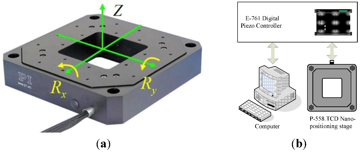
To verify the effectiveness of the state space model and the proposed identification method, experiments were implemented on a commercially-available 3-DOF piezo-actuator-driven stage (P-558.TCD, Physik Instrumente), as shown in Figure 1a. Driven by four piezoelectric actuators, the P558.TCD can generate linear displacements in the vertical direction Z and rotation around two orthogonal horizontal axes R_x and R_y. Table 1 shows the motion range and resolution in each DOF.

Table 1. Motion range and resolution in each degree-of-freedom (DOF)

DOF	Z	Rx	Ry
Motion range	50 μm	±250 μrad	±250 μrad
Resolution	0.5 nm	50 nrad	50 nrad

Table 1. Motion range and resolution in each degree-of-freedom (DOF)

DOF	Z	Rx	Ry
Motion range	50 μm	±250 μrad	±250 μrad
Resolution	0.5 nm	50 nrad	50 nrad

Figure 1. Experimental settings on the piezo-actuator-driven stage: (a) picture and (b) schematic.

Figure 1. Experimental settings on the piezo-actuator-driven stage: (a) picture and (b) schematic.

For displacement measurements, three capacitive sensors built in the stage are employed. All displacements were measured with a sampling interval of 2 ms in the present study. Both the actuators and the sensors in the stage were connected to a host computer via a digital controller (E-761, Physik Instrumente) and controlled through Labview, as shown in Figure 1b. As instructed by its manual, the piezo controller can drive the actuator with a maximum operating frequency of 10-20 Hz if an input voltage in the range of 30–50 V is applied. During operation, the motion of the four piezoelectric elements must be coordinated to reduce the internal forces generated due to the over actuation, which may cause reduced stiffness and even break or damage the piezo-actuator-driven stage. This is realized by a user program interface provided by the manufacturer, which is used to generate the voltage input of each piezoelectric actuator from the user defined reference signal.

3.1. Linearity of the 3-DOF Piezo-Actuator-Driven Stage

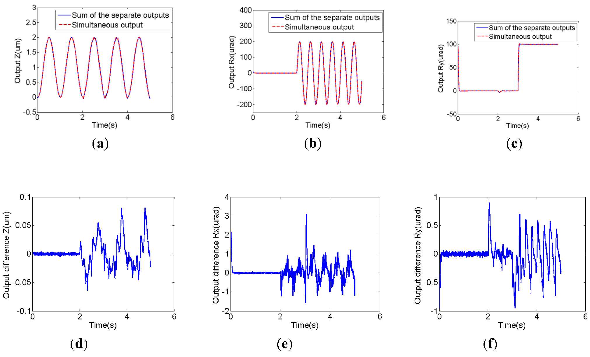
To examine the linearity of the 3-DOF piezo-actuator-driven stage, a case study was conducted prior to the system identification. In particular, a 1 Hz 1 μm sinusoidal reference signal with 1 μm offset, a 2 Hz 200 μm sinusoidal reference signal with 2 s time delay and a 100 μm step reference signal with 3 s time delay were provided to the Z, R_x and R_y channel, respectively, and the corresponding outputs were measured. Then, the stage displacement output, as these three signals were applied simultaneously, was measured. The criterion used for the linearity examination is that if the output with three input signals equals or approximately equals the sum of the outputs when the signals is applied individually, the 3-DOF piezo-actuator-driven stage is linear or can be approximately considered to be linear. Figure 2 shows the comparison between the two outputs mentioned above. It can be seen that they overlapped with each other, indicating that the stage can be approximately considered to be a linear system. Differences between the measured output when the three inputs were provided to the different channels simultaneously and the sum of the outputs when the three inputs were provided separately exist. For example, in the R_x direction, the maximum difference is approximately 3 μm, which is only 1.5% of the amplitude of the reference signal. This difference might be due to the nonlinearities of the 3-DOF piezo-actuator-driven stage, which is ignored in the model development presented in this paper.

Figure 2. Linearity of the 3-DOF piezo-actuator-driven stage: (a–c) comparison between the measured output when the three inputs were provided to the different channels simultaneously and the sum of the outputs when the three inputs were provided separately; (d–f) difference between these two outputs.

Figure 2. Linearity of the 3-DOF piezo-actuator-driven stage: (a–c) comparison between the measured output when the three inputs were provided to the different channels simultaneously and the sum of the outputs when the three inputs were provided separately; (d–f) difference between these two outputs.

3.2. System Identification of the 3-DOF Piezo-Actuator-Driven Stage

Figure 3 shows the flow chart of system identification. Since different signals applied in system identification may lead to the difference in the model identified, the effects of applying the random signal and the chirp signal in the parameter estimation were investigated in the signal selection in this study. The two signals were compared, and the one with less model prediction error was employed as the input for order selection, in which state space models with different orders were identified and compared. The one with less model prediction error was employed as the model for the piezo-actuator-driven stage.

Figure 3. Flow chart of black box system identification.

Figure 3. Flow chart of black box system identification.

For signal selection, a 20 μm reference chirp signal with 20 μm offset and frequency ranging from 1 to 100 Hz was provided to channel 1 (reference Z channel), and the corresponding output in each channel was measured. Based on the empirical knowledge of our previous study on piezoelectric actuators, the order of the state space model was originally set to be three, and in Equation (17) was set to be a zero matrix. Since the covariance of the parameters is unknown, P₀ is set to be a diagonal matrix with big covariance designated in the diagonal elements. By applying online estimation with the identified Hankel matrix, the system matrices of the state space model (Equation (19), I = 1) were obtained.

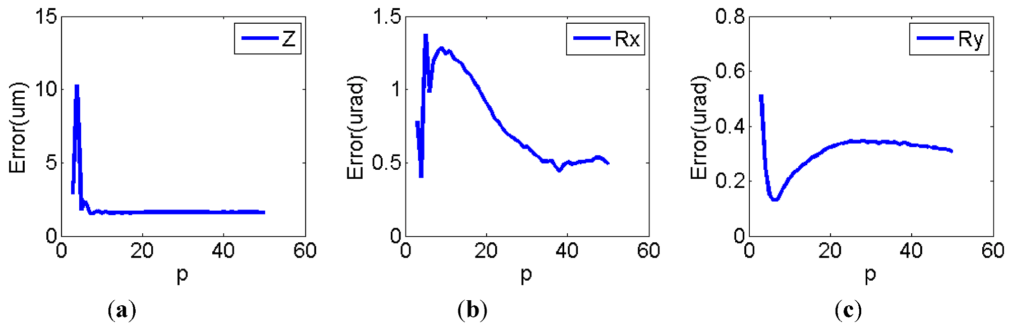
The estimation error varied, depending on the values of parameter p in Equation (2). Figure 4 (a–c) shows the estimated error versus the p-value. It can be seen that if p = 8, the estimation errors in all three output directions approached or reached their individual minimum values. Therefore, it is reasonable to set p = 8, as the chirp signal is provided to channel 1.

Figure 4. Estimation error changes with p-value when reference input was applied in channel (a) Z direction; (b) Rx direction; (c) Ry direction.

Figure 4. Estimation error changes with p-value when reference input was applied in channel (a) Z direction; (b) Rx direction; (c) Ry direction.

For other two channels, a 200 μrad reference chirp signal with frequency ranging from 1 to 100 Hz was applied. By employing the aforementioned procedure, p was set to 25 and 27 for channel 2 and 3 respectively. Table 2 shows the prediction error in each direction, as a 1 Hz sinusoidal reference input was applied to the three channels, respectively. The prediction errors are calculated in terms of the 2-norm of the error vector (defined as the difference between the measurement and the model prediction). It is seen that the diagonal prediction error is 0.1944 μm, 4.864 μrad and 4.3387 μrad in the Z, R_x and R_y direction, respectively, which is 0.49%, 2.43% and 2.16% of the desired movement in the individual direction.

Table 2. Model prediction error if chirp inputs were applied.

Direction	Z (μm)	Rx (μrad)	Ry (ΜRAD)
1 Hz 20 μm sinusoidal inputs with 20 μm offset in channel 1	0.1944	0.4030	0.2008
1 Hz 200 μrad sinusoidal inputs in channel 2	0.0192	4.8640	0.0760
1 Hz 200 μrad sinusoidal inputs in channel 3	0.0263	0.2060	4.3387

Table 2. Model prediction error if chirp inputs were applied.

Direction	Z (μm)	Rx (μrad)	Ry (ΜRAD)
1 Hz 20 μm sinusoidal inputs with 20 μm offset in channel 1	0.1944	0.4030	0.2008
1 Hz 200 μrad sinusoidal inputs in channel 2	0.0192	4.8640	0.0760
1 Hz 200 μrad sinusoidal inputs in channel 3	0.0263	0.2060	4.3387

Similar to the use of the chirp signal, 40 μm and 200 μrad reference random signals were also applied to each channel, respectively. The order of each sub-model was chosen to be three, and p was set to nine, 14 and 13 for the three channels, respectively. The same 1 Hz sinusoidal inputs were provided to difference channels, and the output was measured and compared with the model prediction. Table 3 illustrates the model prediction error. In contrast to the chirp signal, it can be concluded that the model prediction errors is much bigger when random signals are used in the model identification. For example, when a 1 Hz 200 μrad sinusoidal reference input was provided to channel 2, the model prediction error in the R_x direction reached 57.362 μrad by using the random inputs, which is over 10-times larger than that derived by using the chirp signal. As a result, a chirp signal was employed as the reference input for model identification below.

Table 3. Model prediction error if random inputs were applied.

Direction	Z (μm)	Rx (μrad)	Ry (ΜRAD)
1 Hz 20 μm sinusoidal inputs with 20 μm offset in channel 1	0.8670	0.8946	0.2061
1 Hz 200 μrad sinusoidal inputs in channel 2	0.0542	57.362	0.1020
1 Hz 200 μrad sinusoidal inputs in channel 3	0.0624	1.0143	45.9597

Table 3. Model prediction error if random inputs were applied.

Direction	Z (μm)	Rx (μrad)	Ry (ΜRAD)
1 Hz 20 μm sinusoidal inputs with 20 μm offset in channel 1	0.8670	0.8946	0.2061
1 Hz 200 μrad sinusoidal inputs in channel 2	0.0542	57.362	0.1020
1 Hz 200 μrad sinusoidal inputs in channel 3	0.0624	1.0143	45.9597

To determine the order of the state space model, the parameter identification, as described previously, was repeated with varying values of n (Equation (1)) in each channel. Table 4, Table 5, Table 6 show the estimation errors in each channel.

Parameter p was chosen to have different values for varying orders based on the method mentioned above. It can be concluded that if the chirp signal was used in channel 1, the estimation error in the Z direction reached its minimum value of 1.4906 μm with the order of the sub-model being six or seven. For the R_y direction, the optimal choice was to set n = 7. Therefore, the sub-model for channel 1 was considered to be a seventh order state space system. The system matrices were determined as given in Equation (23). Using a similar procedure, the orders of the sub-model for the other two channels were both chosen to be four, and the system matrices were determined, as shown in Equations (24) and (25).

(23)

(24)

(25)

Table 4. Estimation error from the chirp inputs in channel 1.

Order	p	Estimation error
		Z (μm)	Rx (ΜRAD)	Ry (ΜRAD)
2	11	1.5635	1.1174	0.1614
3	8	1.5368	1.2597	0.1631
4	11	1.4936	0.8100	0.3496
5	14	1.4914	0.1876	0.1607
6	31	1.4906	0.1184	0.1238
7	38	1.4906	0.1192	0.0908
8	38	1.4907	0.1180	0.1099
9	38	1.4907	0.1202	0.1031
10	30	1.4912	0.1195	0.1251
11	30	1.4913	0.1186	0.1236
12	28	1.4912	0.1266	0.1180

Table 4. Estimation error from the chirp inputs in channel 1.

Order	p	Estimation error
		Z (μm)	Rx (ΜRAD)	Ry (ΜRAD)
2	11	1.5635	1.1174	0.1614
3	8	1.5368	1.2597	0.1631
4	11	1.4936	0.8100	0.3496
5	14	1.4914	0.1876	0.1607
6	31	1.4906	0.1184	0.1238
7	38	1.4906	0.1192	0.0908
8	38	1.4907	0.1180	0.1099
9	38	1.4907	0.1202	0.1031
10	30	1.4912	0.1195	0.1251
11	30	1.4913	0.1186	0.1236
12	28	1.4912	0.1266	0.1180

Table 5. Estimation error from the chirp inputs in channel 2.

Order	p	Estimation error
		Z (μm)	Rx (μrad)	Ry (μrad)
2	47	0.0118	18.0440	0.0565
3	25	0.0106	17.8752	0.0474
4	42	0.0107	17.7877	0.0476
5	47	0.0128	17.7751	0.0483
6	42	0.0129	17.8071	0.0477
7	42	0.0125	17.8073	0.0480
8	47	0.0133	17.8073	0.0477
9	42	0.0118	17.8179	0.0484
10	39	0.0103	17.8363	0.0479
11	42	0.0120	17.8154	0.0475
12	42	0.0119	17.8166	0.0481

Table 5. Estimation error from the chirp inputs in channel 2.

Order	p	Estimation error
		Z (μm)	Rx (μrad)	Ry (μrad)
2	47	0.0118	18.0440	0.0565
3	25	0.0106	17.8752	0.0474
4	42	0.0107	17.7877	0.0476
5	47	0.0128	17.7751	0.0483
6	42	0.0129	17.8071	0.0477
7	42	0.0125	17.8073	0.0480
8	47	0.0133	17.8073	0.0477
9	42	0.0118	17.8179	0.0484
10	39	0.0103	17.8363	0.0479
11	42	0.0120	17.8154	0.0475
12	42	0.0119	17.8166	0.0481

Table 6. Estimation error from the chirp inputs in channel 3.

Order	p	Estimation error
		Z (μm)	Rx (μrad)	Ry (μrad)
2	41	0.0124	1.0996	16.9180
3	27	0.0108	1.0995	16.7524
4	39	0.0111	1.0994	16.5991
5	41	0.0144	1.1006	16.5917
6	39	0.0109	1.0993	16.6212
7	39	0.0111	1.0996	16.6183
8	39	0.0112	1.0996	16.6183
9	39	0.0112	1.0996	16.6177
10	39	0.0111	1.0996	16.6188
11	39	0.0111	1.0993	16.6184
12	39	0.0111	1.0994	16.1686

Table 6. Estimation error from the chirp inputs in channel 3.

Order	p	Estimation error
		Z (μm)	Rx (μrad)	Ry (μrad)
2	41	0.0124	1.0996	16.9180
3	27	0.0108	1.0995	16.7524
4	39	0.0111	1.0994	16.5991
5	41	0.0144	1.1006	16.5917
6	39	0.0109	1.0993	16.6212
7	39	0.0111	1.0996	16.6183
8	39	0.0112	1.0996	16.6183
9	39	0.0112	1.0996	16.6177
10	39	0.0111	1.0996	16.6188
11	39	0.0111	1.0993	16.6184
12	39	0.0111	1.0994	16.1686

3.3. Model Verification

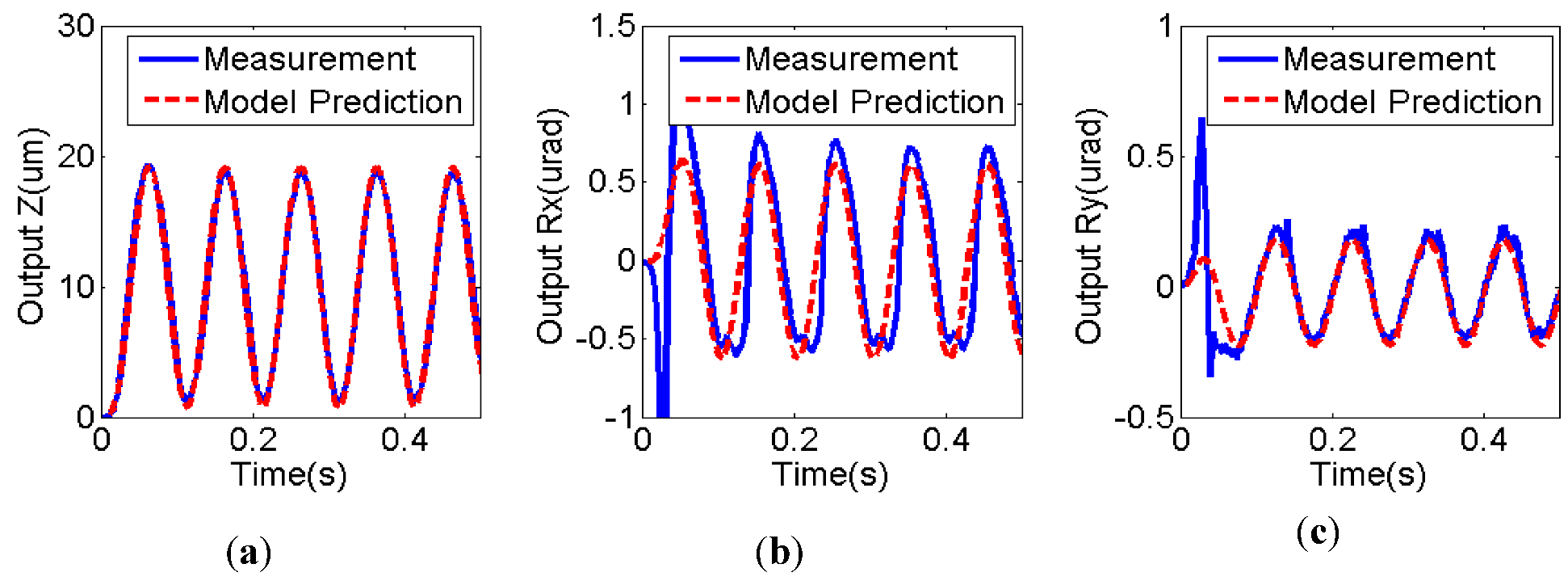
To illustrate the effectiveness of the MAP online estimation method, 1, 5 and 10 Hz sinusoidal reference inputs were provided to different channels, respectively. For comparison, the estimation method introduced in [25] was implemented as well. The parameter p was defined as 21, four and seven, respectively, for the three input channels. Table 7, Table 8 show the prediction error in each direction based on the different identification methods. The prediction errors were calculated in terms of the 2-norm of the error vector, illustrating that the prediction error increases with the frequency.

Table 7. Estimation error by applying the online estimation method.

Input	Channel	Z (μm)	Rx (μrad)	Ry (ΜRAD)
1 Hz 10 μm	1	0.1468	0.1584	0.0642
1 Hz 200 μrad	2	0.0176	1.0305	0.0742
1 Hz 200 μrad	3	0.0196	0.2574	9.9402
5 Hz 10 μm	1	0.3666	0.3743	0.0956
5 Hz 200 μrad	2	0.0538	2.3801	0.2044
5 Hz 200 μrad	3	0.0510	0.2128	3.1906
10 Hz 10 μm	1	0.5296	0.2699	0.0576
10 Hz 200 μrad	2	0.0530	6.3244	0.3327
10 Hz 200 μrad	3	0.0517	1.1101	5.6707

Table 7. Estimation error by applying the online estimation method.

Input	Channel	Z (μm)	Rx (μrad)	Ry (ΜRAD)
1 Hz 10 μm	1	0.1468	0.1584	0.0642
1 Hz 200 μrad	2	0.0176	1.0305	0.0742
1 Hz 200 μrad	3	0.0196	0.2574	9.9402
5 Hz 10 μm	1	0.3666	0.3743	0.0956
5 Hz 200 μrad	2	0.0538	2.3801	0.2044
5 Hz 200 μrad	3	0.0510	0.2128	3.1906
10 Hz 10 μm	1	0.5296	0.2699	0.0576
10 Hz 200 μrad	2	0.0530	6.3244	0.3327
10 Hz 200 μrad	3	0.0517	1.1101	5.6707

In contrast to the identification method introduced in [25], the use of posteriori parameter information in MAP online estimation leads to better estimations on the Hankel matrix. For example, the estimation errors for the 5 Hz, 10 μm sinusoidal inputs to channel 1 were 0.3666 μm, 0.3843 μrad and 0.0956 in the Z, R_x and R_y directions, respectively. These results are 7.3%, 40.6% and 24%, respectively, of those derived using the identification method introduced in [25].

Table 8. Estimation error by applying the identification method introduced in [25].

Input	Channel	Z (μm)	Rx (μrad)	Ry (ΜRAD)
1 Hz 10 μm	1	1.1124	0.9433	0.3675
1 Hz 200 μrad	2	0.0180	2.2639	0.3403
1 Hz 200 μrad	3	0.0374	0.3065	5.3670
5 Hz 10 μm	1	5.0639	0.9224	0.3974
5 Hz 200 μrad	2	0.0541	4.5928	0.3567
5 Hz 200 μrad	3	0.0608	0.6449	11.349
10 Hz 10 μm	1	6.2860	0.9419	0.4139
10 Hz 200 μrad	2	0.0525	17.785	0.2683
10 Hz 200 μrad	3	0.0543	1.0064	13.497

Table 8. Estimation error by applying the identification method introduced in [25].

Input	Channel	Z (μm)	Rx (μrad)	Ry (ΜRAD)
1 Hz 10 μm	1	1.1124	0.9433	0.3675
1 Hz 200 μrad	2	0.0180	2.2639	0.3403
1 Hz 200 μrad	3	0.0374	0.3065	5.3670
5 Hz 10 μm	1	5.0639	0.9224	0.3974
5 Hz 200 μrad	2	0.0541	4.5928	0.3567
5 Hz 200 μrad	3	0.0608	0.6449	11.349
10 Hz 10 μm	1	6.2860	0.9419	0.4139
10 Hz 200 μrad	2	0.0525	17.785	0.2683
10 Hz 200 μrad	3	0.0543	1.0064	13.497

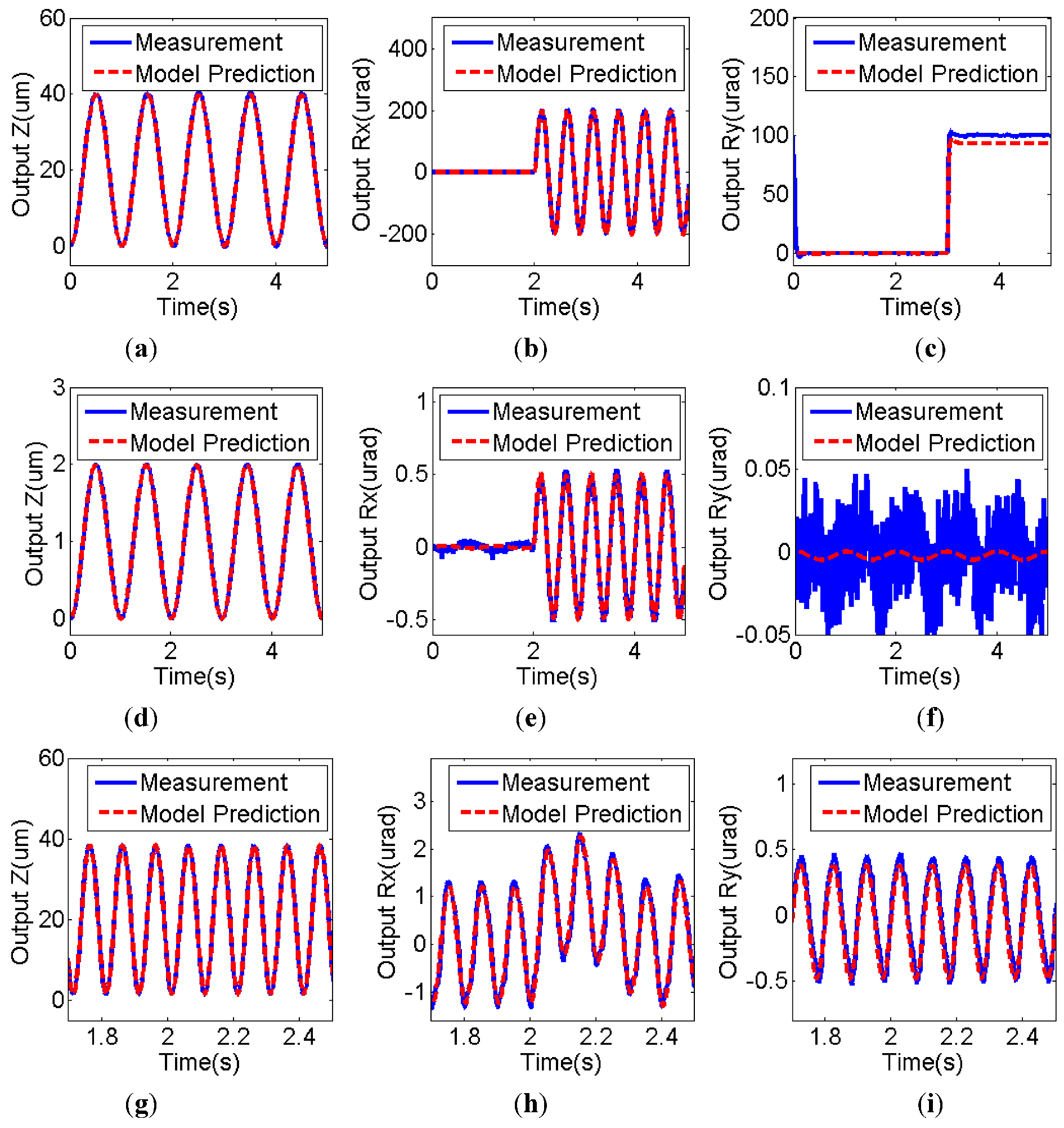
Figure 5 shows the output in each direction as a result of a 10 μm 10 Hz sinusoidal reference input with 10 μm offset in the Z direction compared with the model prediction. It can be clearly seen that the identified state space model is able to describe the coupling effect between each axle.

Figure 5. Comparison of experimental results and model prediction under 10 μm 10 Hz sinusoidal input in channel 1: (a) Z direction; (b) Rx direction; (c) Ry direction.

Figure 5. Comparison of experimental results and model prediction under 10 μm 10 Hz sinusoidal input in channel 1: (a) Z direction; (b) Rx direction; (c) Ry direction.

3.4. Case Study with Combined Inputs

To verify the identified linear state space model with combined inputs, three experiments were implemented. In the first experiment, the reference inputs simultaneously applied to the three channels are a 1 Hz and 20 μm sinusoidal reference with a 20 μm offset, a 2 Hz and 200 μrad sinusoidal reference with a time delay of two seconds and a 100 μrad step input with a time delay of three seconds. The outputs in the three directions were measured, and the predicted outputs were obtained according to the identified state space model of Equations (23–25), respectively. In the second experiment, a 1 Hz and 1 μm sinusoidal input with 1 μm offset and a 2 Hz, 0.5 μrad sinusoidal reference input with a 2 s time delay were provided to the piezo-actuator-driven stage with the third channel kept zero. The outputs were measured and compared to the predicted outputs. To validate the model in high frequency, the input of 1 Hz and 2 μm sinusoid in channel 1 was replaced with a 10 Hz 40 μm one in the third experiment. Also, the corresponding outputs in the three directions were measured and compared to the outputs predicted by the identified state space model. The comparison is shown in Figure 6, from which it can be concluded that the model is able to describe the performance (both dynamics and cross-coupling effect) of the 3-DOF piezo-actuator-driven stage.

Figure 6. Comparison of experimental results and model prediction from combined inputs to all three channels in the first experiment (a–c); in the second experiments (d–f) and in the third experiments (g–i).

Figure 6. Comparison of experimental results and model prediction from combined inputs to all three channels in the first experiment (a–c); in the second experiments (d–f) and in the third experiments (g–i).

4. Conclusions

A straightforward modeling method for multi-DOF piezo-actuator-driven stages is based on the internal configuration by means of physics laws, as reported in the literature [12,13,14,15]. However, such details with regard to the internal structure are often not provided by the manufactures. Therefore, system identification for multi-DOF piezo-actuator-driven stages with unknown configuration is always required for the model development.

The contribution of this paper is the development of a black box model used to describe the dynamics of 3-DOF piezo-actuator-driven stages with unknown physical configuration, which allows the investigation of the complex system performance with unknown physical configuration by means of the linear state space model. By combining the MAP online estimation methods, the Hankel matrix of the state space model was identified and the model parameters were updated as new observations were available. To show the effectiveness of the proposed estimation method, model verification experiments were carried out on the piezo-actuator-driven stage, and the outputs obtained were compared to the predictions of the state space model identified using the method introduced in [25]. From the model verification results, it was shown that the linear state space model can predict the dynamic performance of a piezo-actuator-driven stage with improved accuracy. By making use of the posteriori parameter information, the MAP online estimation method performs better in the model identification than the least squares method. Moreover, the identified parameters are updated online as new and more data becomes available. The developed model and parameter identification methods provide a starting point from which to adaptively compensate for the dynamics and cross-coupling effects of the piezo-actuator-driven stage by means of the mode-based control scheme.