A Compact Ionic Polymer Metal Composite (IPMC) System with Inductive Sensor for Closed Loop Feedback

Abstract

Ionic polymer metal composite (IPMC), of which a low actuating voltage (<5 V), high power efficiency and biocompatibility makes it a proven candidate for low power devices. However, due to its inherent nonlinear behaviour and time-variance, feedback control, as well as reliable sensing means, are required for accurate operations. This paper presents an IPMC actuator implemented with an inductive sensor to enhance the reliability and compactness of the overall device. A practical, low cost and importantly, compact inductive sensor fabricated on a printed circuit board (PCB) is proposed here. Target material selections and coil design considerations are discussed. It is experimentally determined that the inductive sensor has comparable performance to a laser sensor. Based on a proportional-integral-derivative (PID) control results the inductive sensor has demonstrated to be an alternative to a laser sensor allowing devices using IPMC actuators to be compact.

1. Introduction

Ionic polymer metal composite (IPMC) is a smart material requiring low driving voltage (<5 V) with a large displacement. IPMC, usually fabricated in strips, has been implemented in various devices, such as fins of bio-inspired underwater robotics [1], rotary joint [2], microgripper [3], and many others. In particular, its high energy density, high efficiency and low power consumption makes it extremely useful in low power applications [4,5,6]. In general, IPMC is a bending actuator aimed at applications that do not required large force. The typical force generated at the tip of the IPMC as bending actuator is approximately 10 gf for a 45 × 15 × 0.35 mm IPMC strip. The bending deflection can be very large and could extend beyond 90°. Hence, IPMC is a large deflection but low force bending actuator operated with low excitation voltage.

In order to compensate for the nonlinearity and time-variance commonly seen in IPMC driven system [7,8,9], a reliable controller with accurate sensing mechanism tailored to the application’s scenario is needed. The current sensing methods can be summarized into two categories: (i) contact and (ii) non-contact sensors.

Contact sensors, such as a strain gauge [10] or additional IPMC sensing strip [11], are either glued or temporarily attached to the driving IPMC so that the deflection or displacement of IPMC actuator can be precisely measured in a minimum space cost. For example, [10] glued a resistive strain gauge near the fix end of the IPMC where the largest deflection of IPMC occurs and, thus, the tip displacement can be calculated with the strain-to-displacement relationship from an isotropic cantilever beam model. However, any contact sensor will add extra rigidity to the actuator, which is especially crucial for IPMC because of its limited output force (normally several mN) [12]. More importantly, as shown in Figure 1a, the sensor glued at the IPMC base and, hence, the IPMC does not behave like an ideal beam, as the glue causes uneven distributed Young Modulus along the beam. As such no accurate, time-invariant relationship between the strain at the base and tip deflection can be found. The use of another IPMC sensing strip, as reported in [11], as an integrated sensor has the advantages of simplicity, compliant and bio-compatibility, which allows it to be implemented in biomedical applications. In addition, it can be even more compact, compared with the inductive sensor. However, due to its inherent properties, such as dehydration, hysteresis, and non-linearity, the accuracy of its sensing largely depends on the environmental stability rather than the sensor itself. Hence, these negate the advantages of using another IPMC as a sensor.

Figure 1. Schematic of (a) strain gauge and (b) laser gauge sensors.

Figure 1. Schematic of (a) strain gauge and (b) laser gauge sensors.

Non-contact sensors include laser sensors [2,6] and digital cameras (CMOS or CCD) [13,14]. Laser sensor is by far the most accurate and widely used distance sensor not only in IPMC but many other academic and industrial applications. The resolution of a laser sensor is typically several μm with a flexible sensing range (~10 mm) able to be programed with wide bandwidth up to a few kHz. Most laser sensors use the triangulation measurement principle (Figure 1b) to detect the distance change. The laser beam is projected onto the target and reflected into a collection lens, which focuses an image of the spot on a linear array camera. The position of the spot image on the pixel of the camera is then processed to determine the distance to the target. However, though non-contact sensors have many advantages compared with contact ones, there is one key obstacle that limits them from truly being applied in portable applications; their bulky size. Normally, the dimension of either laser sensor or digital camera is about 10 cm, and a sensing range of several more cm is also required, which makes the overall size even larger, as shown in Figure 1b. Therefore, a compact, non-contact sensing method would obviously be a better choice.

In this paper, an inductive sensor in a printed circuit board (PCB) form is proposed as a compact proportional-integral-derivative (PID) feedback sensor for IPMC displacement control. It removes the need for rigid contact (e.g., strain gauge) or bulky non-contact (e.g., laser) sensors and ensures the portability and reliability of the overall systems. Aside from being compact, these sensors must have low power consumption, low cost and sufficient high resolution and bandwidth.

The principle of inductive sensing is first discussed followed by the sensor’s target material selection and then the PCB coil design. The performance of the inductive sensor is later evaluated. It is compared with a laser sensor in measuring an IPMC’s deflection, driven by a chirp signal, to determine its bandwidth and the frequency response of IPMC. Finally, a PID controller is implemented to test the inductive sensor as the feedback loop in controlling the IPMC’s deflection.

2. Inductive Sensing Principle

An AC current flowing through a coil will generate an AC magnetic field and at this time the coil has its own frequency-depended equivalent resistance (R_s) and inductance (L_s). If a conductive material, e.g., a metal plate, is brought into the vicinity of the coil, this magnetic field will induce circulating (eddy) current on the surface of the target. This eddy current is a function of the distance, size and composition of the target and in return generates their own magnetic field, which opposes the original field generated by the sensor coil as shown in Figure 2. Therefore, the changes in the equivalent resistance (R(d)) and inductance (L(d)) can be viewed as distant-dependent components. Once the target and AC driving voltage are identified, R(d) and L(d) have their exclusive relationship with the distance and thus could be used as a distance sensor.

With a LDC1000 inductance-to-digital converter integrated circuit, the equivalent resistance of the sensor coil is measured by monitoring the energy dissipation of the resonance circuit and the inductance is measured by measuring the oscillation frequency of the resonance circuit (a parallel capacitor is usually added to the sensor coil to create a resonator and, thus, reduce the energy consumption).

Figure 2. Inductive sensing principle.

Figure 2. Inductive sensing principle.

2.1. Target Material Selection

Since the sensing mechanism is based on the electromagnetic coupling between the coil and the conductive target, the physical characteristics (mainly resistivity and magnetic permeability), shape and dimension of the conductive target have great influences on the sensor’s performance. Generally, inductive sensors have better performance detecting a low resistivity, ρ and low permeability, µ target. In addition, the coating uniformity of the target has an effect on the performance in measuring a rotating or moving target. Low resistivity and low permeability metals, such as copper and aluminum, are, hence, good candidates. Penetration depth is another consideration worth noting in the target selection. As the eddy currents flow beneath the surface of the conductive target, there is a phenomenon where its density reduces exponentially with depth, which is called the skin effect. Table 1 summarizes the resistivity and penetration depth of several materials under normal working frequencies. The thickness of the target has to be greater than some certain limits otherwise the magnetic field generated by eddy currents may not be large enough for measurable coupling. For example, if a stainless steel plate is measured by an inductive sensor whose resonance frequency is 1 MHz, the thickness must be at least 440 µm or greater, otherwise the magnetic coupling would be too weak due to the skin effect and difficult to detect.

Table 1. Resistivity and penetration depth of typical target materials [15].

Metal	Resistivity (10−6 Ω·m)	Penetration Depth (µm)
		10 kHz	100 kHz	1 MHz	10 MHz
Copper	0.017	660	210	66	21
aluminium	0.026	820	260	82	26
Stainless steel	0.77	4400	1400	440	140
Titanium alloy	1.69	6600	2100	660	210

Table 1. Resistivity and penetration depth of typical target materials [15].

Metal	Resistivity (10−6 Ω·m)	Penetration Depth (µm)
		10 kHz	100 kHz	1 MHz	10 MHz
Copper	0.017	660	210	66	21
aluminium	0.026	820	260	82	26
Stainless steel	0.77	4400	1400	440	140
Titanium alloy	1.69	6600	2100	660	210

2.2. PCB Coil Design

Here, the coil is made of copper in a PCB form, which does not only electrically connect components but provide mechanical supports. This kind of flat coil has several advantages compared with other coils in the ease of manufacturing, low cost and reliability, albeit a larger size is needed.

The resonant frequency f_R of a LC circuit, which relates to the distance between the coil and the target is proportional to the energy dissipation that relies on the equivalent resistance. Therefore, to design a PCB coil, the following parameters should be considered:

(1) Generally, a coil with a larger outer diameter r_o produces a wider spread magnetic field but with a smaller gradient of magnetic flux density, which makes it less sensitive to the distance change. A typical criterion is to set r_o more than two times of the maximum distance and set inner diameter r_i less than 1/3 of r_o.

(2) The number of coil turns is another notable consideration as it could increase the detection resolution. However, once r_o is decided, the coil turns would be constrained by the PCB’s size (number of layers N, minimum width of trace and gap p, etc.). Therefore, the maximum number of coil turns in one layer is:

$$n_1\approx \frac{r_o-r_i}{2p-1}$$

(1)

(3) The inductance of the coil when there is no conductive target in the vicinity can be estimated by

$$L=7.88\cdot \frac{{\left(r_o+r_i\right)}^2{n_1}^2{N}^2}{13r_o-7r_i}\begin{array}{cc}& \left(\mu H\right)\end{array}$$

(2)

The total capacitance consists of two parts: the trace capacitance (C_t) and the interwoven capacitance (C_IWC, exist only in multilayer PCB coil). C_t can be calculated by the material specification and C_IWC usually equals to ¼ of the capacitance considering two layer traces as parallel metal plates:

$$C_{IWC}=\frac{1}{4}\frac{{\epsilon }_r{\epsilon }_{0}A}{h}=\frac{1}{4}\frac{{\epsilon }_r{\epsilon }_0\pi (r_o^2-r_i^2)}{h}$$

(3)

where ${\epsilon }_r$ is the relative permittivity constant, ${\epsilon }_r$ is the vacuum permittivity and h is the distance between two layers.

(4) Then the self-resonance frequency (SRF) is:

$$SRF=\frac{1}{2\pi \sqrt{L(C_t+C_{IWC})}}$$

(4)

The maximum inductance as given in Equation (2), it is usually two times of the minimum inductance; hence, the minimum resonance frequency f_min is half the maximum resonant frequency, f_max and less than 1/6 of SRF (in case of the mutual inductance between coil trace and wires).

$$f_{\min }=\frac{1}{2\pi \sqrt{LC}}=\frac{1}{2}{f}_{\max }\le SRF/6$$

(5)

where C is the overall capacitance of the parallel resonator, L is the result of Equation (2). Equation (5) can be used to calculate the parallel capacitor to operate at the desired frequency.

(5) The DC resistance of a PCB coil is given by the basic resistivity equation:

$$R_{DC}=\frac{l}{wt}\rho =n_1\left[\frac{\pi (r_o+r_i)}{wt}\right]\rho N$$

(6)

where $\rho$ is the resistivity, l, w and t are the length, width and thickness of trace, respectively. Due to the skin effect, the worst AC resistance would be two times the DC resistance:

$$R_{AC}=2R_{DC}$$

(7)

Therefore, the Q factor of a no load (no conductive target in the vicinity) coil is:

$$Q=\frac{2\pi f_{\min }L}{R_{AC}}$$

(8)

Q factor is regarded as a general determining factor of inductive sensors’ performance (resolution, linearity, robustness). Therefore, increasing it will enhance the performance of inductive sensors. For example, if a four-layer PCB is used instead of two, the capacitance would be four times greater, while the resistance would only be doubled, which leads to a doubling of the Q factor.

Hence, four PCB coils with different diameters will be constructed (two layers PCB, 0.004 inches width and gap, 1 oz copper trace). All the inner diameters are set to 2 mm as it is the minimum diameter able to be printed to accommodate as many turns as possible. From the parameters summarized in Table 2, it is expected that coil 4 has the highest Q factor. However, it has to be mentioned that the Q factor only denotes the best-sensing performance the coil could achieve regardless of the distance to the target. Therefore, its performance, in terms of resolution, linearity, and detection range, needs to be quantified to determine the most suitable coil design.

Table 2. Inductive parameters of four designed PCB coils.

Number	Outer Diameter (mm)	Inner Diameter (mm)	Turns	Free Field Frequency (kHz)	Free Field Inductance (uH)	Parallel Capacitance (pF)	Q Factor
1	3.61	2	85	100	376.39	67.29	5.51
2	2.61	2	60	360	139.56	14	6.5
3	2.29	2	52	360	94.53	20.67	11
4	1.97	2	44	500	58.49	17.32	17

Table 2. Inductive parameters of four designed PCB coils.

Number	Outer Diameter (mm)	Inner Diameter (mm)	Turns	Free Field Frequency (kHz)	Free Field Inductance (uH)	Parallel Capacitance (pF)	Q Factor
1	3.61	2	85	100	376.39	67.29	5.51
2	2.61	2	60	360	139.56	14	6.5
3	2.29	2	52	360	94.53	20.67	11
4	1.97	2	44	500	58.49	17.32	17

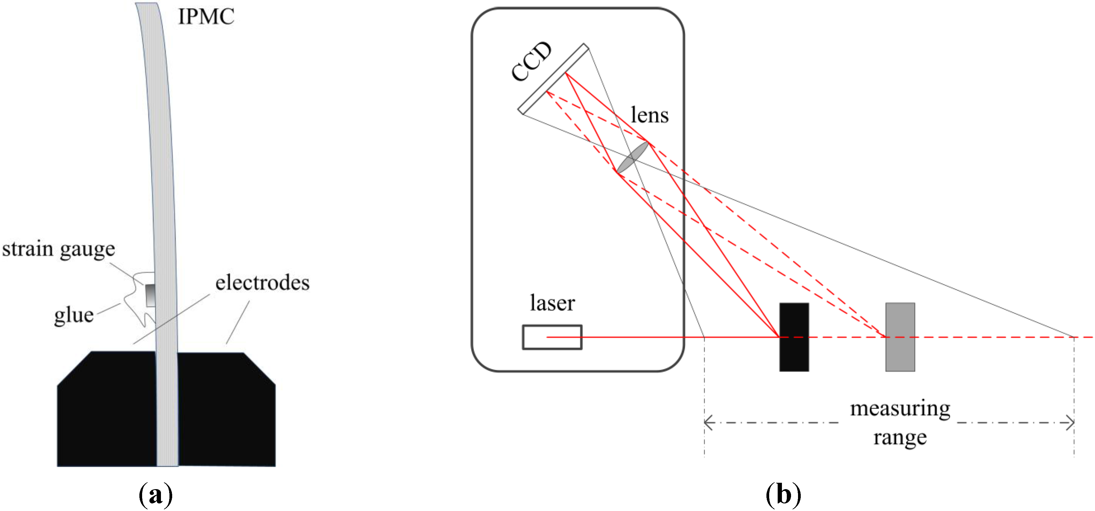
3. Performance of the Inductive Sensor

There are several parameters determining the performance of the inductive sensor, such as resolution, linearity, and frequency response. Here, these parameters will be experimentally determined.

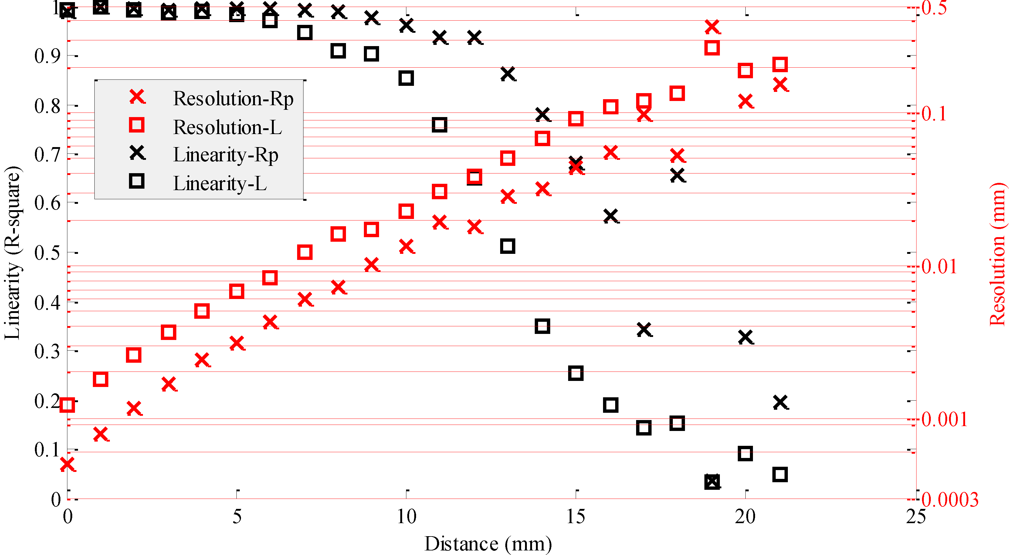
3.1. Resolution and Linearity of Inductive Sensors

As mentioned in previous section, the inductive sensor connected to LDC1000 can generate two independent outputs, inductance L and resistance Rp that are computed from the LDC1000’s Y output. Here a linear motor E43K4U-05-120 whose minimum step size is 1.5 µm and an anti-backlash nut both from Haydonkerk are used to move a conductive target along a linear path with a constant velocity to determine the resolution and linearity of the inductive sensor. A 12.5 × 5 × 0.035 mm conductive copper tape serving as the sensor target is attached at the end of the moving plastic rod motorised by the linear motor. It has to be noted that the thickness of the commercially available tape used is thinner than the penetration depth given in Table 1. Therefore, the sensing performance would deteriorate to some extent and it is believed that using a thicker tape would definitely improve the sensing performance. The target is initially placed close to the centre of the PCB coil and then driven away with a speed of 0.1 mm/s by the linear motor. The output of Rp and L are recorded and plotted in Figure 3. It has to be noted that the LDC1000 does not directly output the equivalent resistance but a proximity data, Y, which has to be converted with the taught Rp range to obtain the real equivalent resistance. The converting relationship is as following:

$$Rp=(R{p}_{MAX}\times R{p}_{MIN})/(R{p}_{MIN}\times (1-Y)+R{p}_{MAX}\times Y),\begin{array}{cc}& \begin{array}{cc}in& \mathrm{\Omega }\end{array}\end{array}$$

(9)

in which Rp_MAX and Rp_MIN are the taught Rp limits.

Figure 3. Rp and L results measuring a linear moving target.

Figure 3. Rp and L results measuring a linear moving target.

From Figure 3, both Rp and L have a sharp rate of change initially when the distance is small and gradually reduces as the target moves away. The slope of the plot in a sense denotes the resolution of the sensor. For example, Rp decreases quickly in the first 5 mm then remains almost constant in the last 5 mm, which means that it has a smaller resolution when it is closer to the target and becomes larger as the distant increases. In addition, non-linearity, which is unwanted in most sensors, is observed in both Rp and L. Therefore, a quantitative computation has to be carried out to compare their performance and determine a suitable working range.

The computation process is as following. The resolution of a sensor is measured by the corresponding distance of the moving target when the least significant digital of output is changed by 1 bit. However, due to the existence of noise, this proves to be difficult. Hence, a “least squares best fit straight line” method is used for a distant increase of 1 mm to determine the linearity of the sensor. The outputs of inductive sensor are fitted with 1st order polynomial function in MATLAB and the R-Square defined in Equation (10) can be regarded as the parameter representing the linearity of an output. R-Square can take on any value between 0 and 1, with a value closer to 1 indicating that a greater proportion of variance is accounted for by the model, i.e., it is more linear.

$$R-square=\frac{{\displaystyle \sum _{i=1}^n{({\widehat{y}}_i-\overline{y})}^2}}{{\displaystyle \sum _{i=1}^n{(y_i-\overline{y})}^2}}$$

(10)

Figure 4. Resolution and Linearity of the outputs of coil 1.

Figure 4. Resolution and Linearity of the outputs of coil 1.

Figure 4 is the computed resolution and linearity of Rp and L. From the figure, both Rp and L have good linearity (black lines) when the distance is <13 mm as their R-square factors are all larger than 0.5. When the distance is greater than 15 mm, the model starts to become inaccurate. On the other hand, the Rp and L resolutions (red lines) deteriorate exponentially as the distance increases. When the target is initially very close to the coil, the resolution can be as small as 1 um and is even better than that of a laser sensor. However, the resolution exponentially increases to about 10 µm when the target is ~10 mm away. Beyond 15 mm, the resolution becomes too large (>60 μm) for most applications. Therefore, coil 1 is suitable to sense distant up to 10 mm. Additionally, in general, the Rp is found to have a slightly better performance with a higher linearity and smaller resolution compared to L.

Table 3. Resolution and Linearity of Rp and L measuring a target at 10 mm distance.

Coil Number	Resolution-Rp	Resolution-L	Linearity-Rp	Linearity-L
1	0.013	0.02	0.96	0.85
2	0.015	0.02	0.95	0.82
3	0.03	0.035	0.95	0.88
4	0.031	0.032	0.94	0.84

Table 3. Resolution and Linearity of Rp and L measuring a target at 10 mm distance.

Coil Number	Resolution-Rp	Resolution-L	Linearity-Rp	Linearity-L
1	0.013	0.02	0.96	0.85
2	0.015	0.02	0.95	0.82
3	0.03	0.035	0.95	0.88
4	0.031	0.032	0.94	0.84

Other 3 coils are also similarly tested and Table 3 summarized their resolution and linearity at a sensing distance of 10 mm. Although the Q factor of coil 4 is the largest according to Table 2, it has the worst resolution. This may be due to the sensing range and the coil diameter, which has a significant impact on the size of the generated magnetic field. If the coil diameter is too small as in coil 4, the generated magnetic field is very weak beyond 10 mm and cannot offer an effective coupling to be sensed. Coil 1 and 2 have better resolutions than 3 and 4 in both Rp and L, while Rp seems to be a more accurate than L in all of 4 coils. Hence, from here onwards, coil 2 will used in the following experiment.

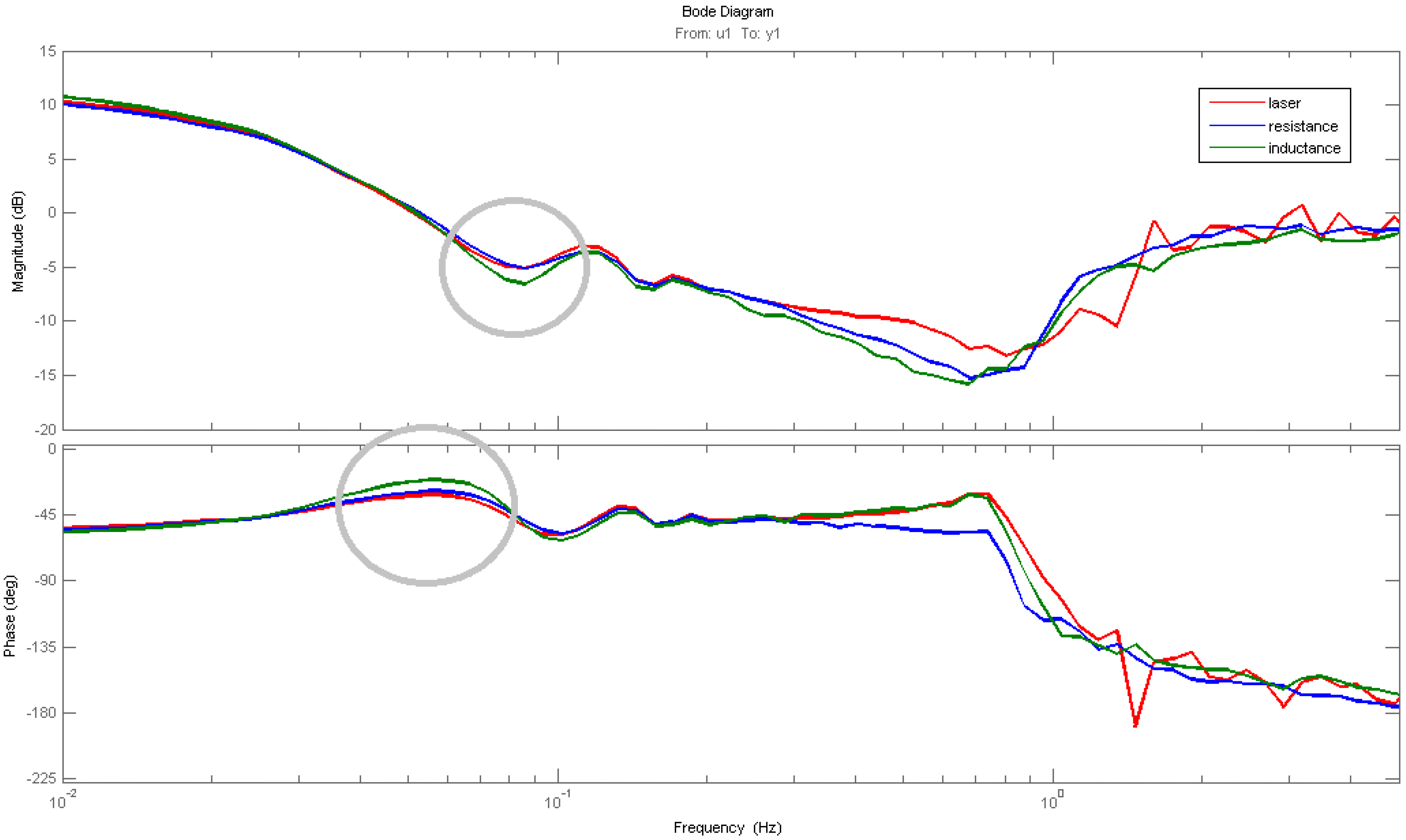
3.2. Measuring IPMC Frequency Response Driven by a Chirp Signal

Bandwidth is another important parameter as it defines the detectable frequency range of the sensor. To measure the bandwidth of the inductive sensor, the PCB coil and a laser sensor are placed on each side of an IPMC driven under a chirp signal whose amplitude is ±2 V and frequency sweep up to 2 Hz. A plastic holder is used to clamp the IPMC and inductive sensor with a gap of 10 mm between them as illustrated in Figure 5a,b. A copper tape with same dimension as described in Section 3.1 is placed at the free end of IPMC cantilever (Figure 5c). Hence, the actual measurement position is 2.5 mm from the free end.The results are acquired under a sampling rate of 100 Hz and plotted in Figure 6. Although the results are in time domain, the mathematical model of the system can still be identified as all the frequency components are contained in the chirp input signal. The results are normalized to 1 to ignore the absolute deflection and then imported into MATLAB to determine the frequency response of IPMC using the system identification toolbox. A mathematical model is necessary to control the IPMC with a feedback loop.

Figure 5. (a) Schematic, (b) a picture of the set-up, and (c) IPMC with conductive tape.

Figure 5. (a) Schematic, (b) a picture of the set-up, and (c) IPMC with conductive tape.

Figure 6. Input and measured outputs of laser and inductive sensors.

Figure 6. Input and measured outputs of laser and inductive sensors.

Figure 7. Bode diagram of IPMC calculated with the outputs of laser and inductive sensors.

Figure 7. Bode diagram of IPMC calculated with the outputs of laser and inductive sensors.

Clearly, from Figure 7, both of Rp and L outputs reasonably match well with the laser sensor over most of the frequency range. However, clear discrepancies could still be found near 0.9 Hz where Rp has a dissimilar phase delay to that of the laser sensor and L output. However, Rp exhibits a slightly better performance than L at about 0.07 Hz (grey circles), as with the results in Figure 4 and Table 3. Also, unlike strain gauge reported in [10], no phase shifting phenomenon is found in low frequency range.

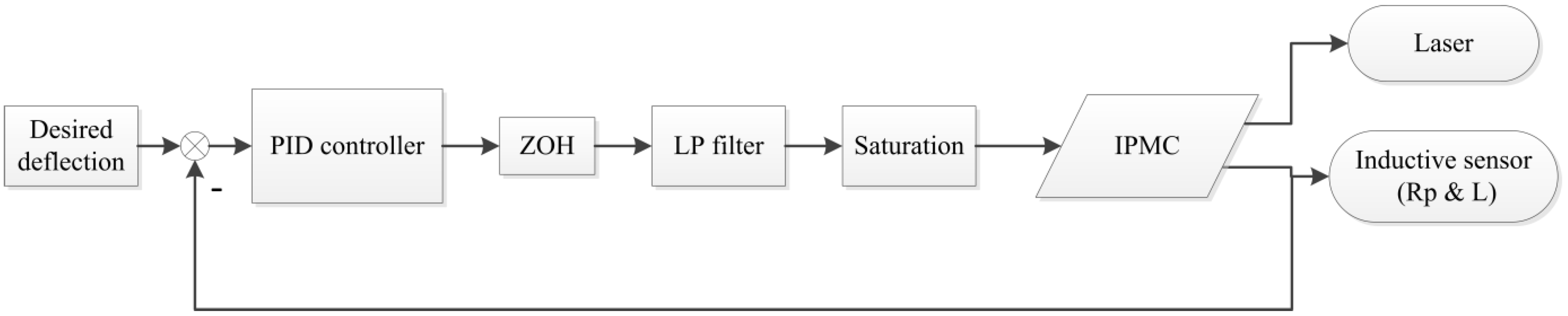
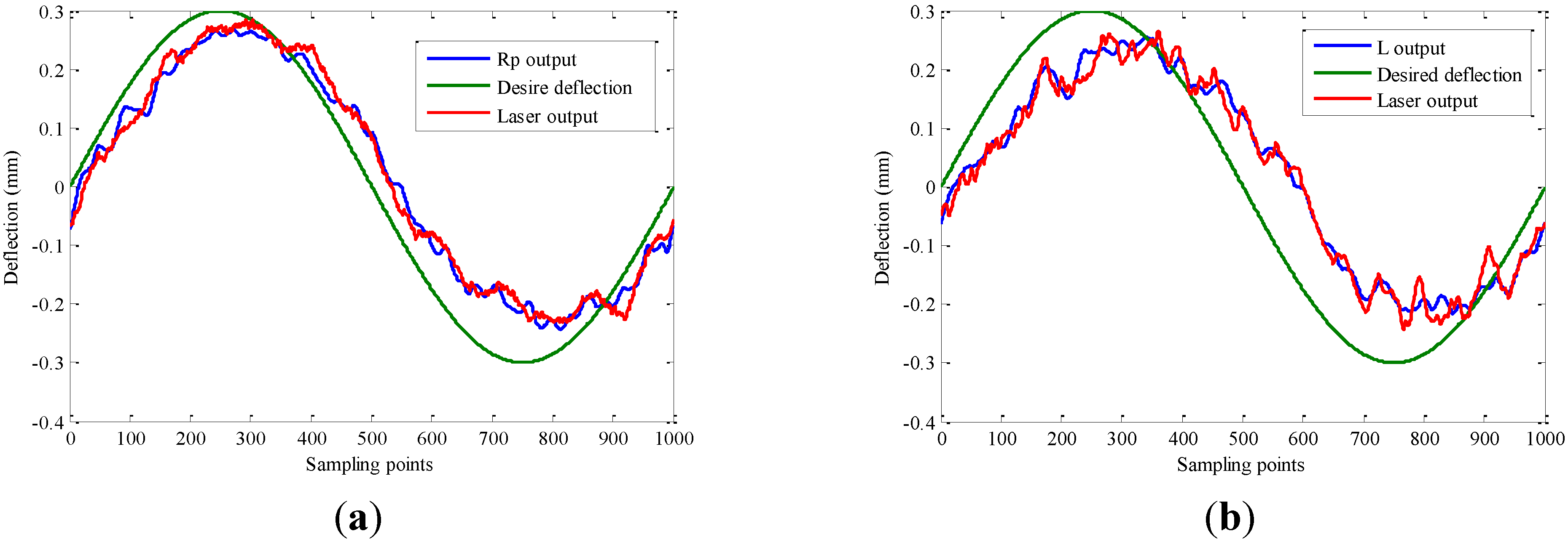
4. IPMC Deflection Controlled by a PID Controller

In this section, the inductive sensor is used in the feedback loop of a PID controller to demonstrate its feasibility and comparable performance with a laser sensor. PID is a well-known three-term controller for industrial applications. It provides a proportional term, an integration term and a derivative term, which controls the attempts to minimize the present error, accumulated past errors and predicted future errors respectively. By tuning the weightings of these three terms, the controller is able to provide control action tailored for specific process requirements and is regarded to be the best controller in history [16]. In addition, there are several adaptive or non-linear tuning methods based on PID, which may account for the time-variant or non-linearity properties of IPMC [16,17]. However, since the aim is to demonstrate the use of PCB inductive sensor as a compact sensor for controlling the deflection of the IPMC, only PID will be used to demonstrate this feasibility. Figure 8 illustrates the block diagram of a PID controller for the IPMC with the inductive sensor as the feedback loop. The laser sensor is only used to measure the deflection for comparison and is not part of the feedback loop.

Figure 8. Block diagram of the PID controlled IPMC deflection system.

Figure 8. Block diagram of the PID controlled IPMC deflection system.

The desired excitation voltage to the IPMC follows a ±0.3 V sine wave with a frequency of 0.1 Hz. The LP (low-pass) filter is chosen to be $Q(s)=\raisebox{1ex}{$50$}\!\left/ \!\raisebox{-1ex}{$(s+50)$}\right.$, whose cut-off frequency is 8 Hz to eliminate the high frequency non-mechanical noise. Also, a limit of ±2 V is added to clamp the controller output voltage so as not to damage the IPMC. However, due to the existence of this limit, the controller may output oscillating signal if the controller output is saturated at 2 V and it could be amplified and result in the IPMC oscillating. The controller parameters are chosen according to [2], enabling a true comparison. The presence of noise, as well as the microscopic targeted displacements constraint the output’s signal to noise ratio, which makes it unrealistic to implement a derivative term, as it would amplify the noise. Therefore, in this experiment, K_d = 0, K_P = 9 and K_I = 2.75 are chosen as the controller parameters. Figure 9a,b shows the measuring results of IPMC deflection with Rp and L as feedback, respectively.

Figure 9. Measured deflection from laser and inductive sensors with Rp (a) and L (b) as feedback loop.

Figure 9. Measured deflection from laser and inductive sensors with Rp (a) and L (b) as feedback loop.

Figure 9 successfully demonstrates the feasibility of using the inductive sensor (Rp and L) as feedbacks for controlling IPMC deflection. The actual deflection as measured by the laser sensor follows the waveform shape well although a clear delay is observed. This is mostly because of the K_d that predicts the future error and is set to 0 here. Choosing K_d is a trade-off, which on one hand could reduce the delay (increasing K_d) and on the other hand would eliminate the oscillation (decreasing K_d). However, in this experiment, although K_d is set to 0, the oscillation still gets amplified. Nevertheless, the results obtained here demonstrated that the inductive sensor can be a suitable candidate to be used for closed loop control of an IPMC actuator.

5. Conclusion

This paper discussed the application of inductive sensors made in a PCB form used as a displacement sensor to control the bending deflection of an IPMC actuator. In contrast to a strain gauge, this sensor is contactless and in addition the sensing distance is greatly reduced compare to a laser sensor. This sensor allows a compact and low cost system using IPMC as an actuator.

References

1. Hubbard, J.J.; Fleming, M.; Palmre, V.; Pugal, D.; Kim, K.J.; Leang, K.K. Monolithic IPMC fins for propulsion and maneuvering in bioinspired underwater robotics. IEEE J. Ocean. Eng. 2014, 39, 540–551. [Google Scholar] [CrossRef]
2. Liu, D.; McDaid, A.; Aw, K.; Xie, S. Position control of an ionic polymer metal composite actuated rotary joint using iterative feedback tuning. Mechatronics 2011, 21, 315–328. [Google Scholar] [CrossRef]
3. Ford, S.; Macias, G.; Lumia, R. Single active finger IPMC microgripper. Smart Mater. Struct. 2015, 24. [Google Scholar] [CrossRef]
4. Amirouche, F.; Zhou, Y.; Johnson, T. Current micropump technologies and their biomedical applications. Microsyst. Technol. 2009, 15, 647–666. [Google Scholar] [CrossRef]
5. Lee, S.; Kim, K.J. Design of IPMC actuator-driven valve-less micropump and its flow rate estimation at low Reynolds numbers. Smart Mater. Struct. 2006, 15. [Google Scholar] [CrossRef]
6. McDaid, A.J.; Aw, K.C.; Haemmerle, E.; Xie, S.Q. Control of IPMC actuators for microfluidics with adaptive “online” iterative feedback tuning. IEEE/ASME Trans. Mechatron. 2012, 17, 789–797. [Google Scholar] [CrossRef]
7. Fang, Y.; Tan, X.; Alici, G. Robust adaptive control of conjugated polymer actuators. IEEE Trans. Control Syst. Technol. 2008, 16, 600–612. [Google Scholar] [CrossRef]
8. Kang, S.; Shin, J.; Kim, S.J.; Kim, H.J.; Kim, Y.H. Robust control of ionic polymer–metal composites. Smart Mater. Struct. 2007, 16. [Google Scholar] [CrossRef]
9. Shan, Y.; Leang, K.K. Frequency-weighted feedforward control for dynamic compensation in ionic polymer–metal composite actuators. Smart Mater. Struct. 2009, 18. [Google Scholar] [CrossRef]
10. Leang, K.K.; Shan, Y.; Song, S.; Kim, K.J. Integrated sensing for IPMC actuators using strain gages for underwater applications. IEEE ASME T. Mech. 2012, 17, 345–355. [Google Scholar] [CrossRef]
11. Bonomo, C.; Fortuna, L.; Giannone, P.; Graziani, S. A sensor-actuator integrated system based on ipmcs [ionic polymer metal composites]. In Proceedings of IEEE Sensors, Vienna, Austria, 24–27 October 2004; pp. 489–492.
12. Hao, L.; Sun, Z.; Li, Z.; Su, Y.; Gao, J. A novel adaptive force control method for IPMC manipulation. Smart Mater. Struct. 2012, 21. [Google Scholar] [CrossRef]
13. Ruiz, S.; Mead, B.; Palmre, V.; Kim, K.J.; Yim, W. A cylindrical ionic polymer-metal composite-based robotic catheter platform: Modeling, design and control. Smart Mater. Struct. 2015, 24. [Google Scholar] [CrossRef]
14. Mead, B.; Ruiz, S.; Yim, W. In Closed-loop control of a tube-type cylindrical IPMC. Proc. SPIE 2013, 8687. [Google Scholar] [CrossRef]
15. Wilson, J.S. Sensor Technology Handbook; Elsevier: Oxford, UK, 2004. [Google Scholar]
16. Dorf, R.C.; Bishop, R.H. Modern Control Systems; Addison Wesley: Menlo Park, CA, USA, 1998. [Google Scholar]
17. McDaid, A.; Aw, K.; Xie, S.; Haemmerle, E. Gain scheduled control of IPMC actuators with ‘model-free’ iterative feedback tuning. Sens. Actuators A. Phys. 2010, 164, 137–147. [Google Scholar] [CrossRef]