A Generalized Unbiased Control Strategy for Radial Magnetic Bearings

Abstract

The present work extends a method of unbiased control originally developed for three-pole radial magnetic bearings into a generalized unbiased control strategy that encompasses bearings with an arbitrary number of poles. By allowing the control of bearings with more than three poles, the applicability of the approach is broadened to the case of large rotors. Other ramifications of this generalized unbiased control strategy are fault tolerant unbiased bearings, control of bearings with more than three poles using 3-phase drives, and a novel approach to the unbiased control of eight-pole magnetic bearings.

1. Introduction

In [1], an unbiased control strategy was presented that enables a three-pole magnetic bearing to be controlled with a 3-phase motor drive. The approach converts the current-to-force relationship for a three-pole bearing to a simple complex-valued expression that is straightforward to invert. Other works experimentally demonstrated the viability of the control approach [2,3].

However, the use of the control approach has been limited because three-pole bearings are primarily applicable to the suspension of very small rotors, for example as described in [4]. For very small magnetic bearings, it is difficult to get enough amp-turns around any one pole to get high flux density in the gap. Three-pole bearings are a good solution in this case because they minimize the number of poles for which amp-turns must be provided. Since the peak achievable flux density in the gap may be far less than the saturation flux density of the material for small bearings, small bearings typically have pole tips that are wider than the pole root. A typical small bearing example is shown below as Figure 1. The bearings have an 0.25" rotor outer diameter, an 0.6" stator outer diameter, a 0.005" air gap length, and 50 turns of American Wire Gauge (AWG) 30 magnet wire per pole. In the short-term max force case where the wire is carrying 1A (20 A/mm${}^2$ in the wire cross-section), the peak flux density in the air gap is about 0.5 T, and the peak flux density in the pole root is about 1.4 T.

For larger bearings, the coil cross-section grows with the square of scaling factor, so it is not as difficult to achieve the magnetomotive force needed to drive flux across the gap at saturation levels. In that case, the tooth tip width is the same as the tooth root width, leading to very wide teeth and a very thick back iron for a three-pole geometry.

For larger bearings, a higher pole count is necessary to minimize back iron thickness and optimize bearing size. The present work extends the method of unbiased control considered in [1,2,3] (which only applies to three-pole magnetic bearings) to encompass radial magnetic bearings with an arbitrary number of poles, such as the nine-pole bearing pictured in Figure 2.

Other ramifications of this generalized unbiased approach are addressed in this work, including control of bearings with more than three poles using 3-phase drives and fault tolerant unbiased bearings.

2. Generalized Unbiased Control Problem

For this work, the effects of flux leakage and fringing are assumed negligible, as are eddy current effects and core reluctance. Under these assumptions, a generalized derivation of the relationship between coil currents and force is presented in [5]. The nomenclature from [5] is also used here, as applicable. From [5], the relationships between current and force for a heteropolar magnetic bearing can be represented as

$$\begin{array}{ccc}\hfill F_x& =& {\mathit{I}}^T{\mathit{X}}_x\mathit{I},\hfill \end{array}$$

(1)

$$\begin{array}{ccc}\hfill F_y& =& {\mathit{I}}^T{\mathit{X}}_y\mathit{I},\hfill \end{array}$$

(2)

where $\mathit{I}$ is a vector consisting of the m independently controlled currents in the coils, and ${\mathit{X}}_x$ and ${\mathit{X}}_y$ are indefinite $m\times m$ matrices.

To represent both parts of the force in one non-dimensionalized quantity, complex-valued force, f, is defined where the real part of f corresponds to the x-direction force and the imaginary part corresponds to the y-direction

$$f=\left(\frac{{\mu }_o}{A{B}_{sat}^2}\right)\left(F_x+j{F}_y\right),$$

(3)

where A, $B_{sat}$, and ${\mu }_o$ denote the pole surface area, saturation flux density, and permeability of free space, respectively.

As in [5], there is a mapping matrix between a reduced set of currents, i, and the full set of currents, $\mathit{I}$, intended to simplify the inversion of the relationship between current and force. This mapping is embodied by matrix $\mathit{W}$, an $m\times 2$ matrix of real numbers. In this case, the reduced set of currents is a single complex number, which can be represented by its real and imaginary parts as

$$i=i_r+j{i}_i.$$

(4)

The mapping between reduced currents and the full current vector is defined to be

$$\mathit{I}=\left(\frac{g{B}_{sat}}{{\mu }_{o}N}\right)\mathit{W}\left\{\begin{array}{c}{i}_r\\ i_i\end{array}\right\},$$

(5)

where g and N represent the nominal air gap length and the number of turns per pole, respectively. Matrix $\mathit{W}$ and current i are non-dimensional quantities. Substituting Equations (1) and (5) into Equation (3) yields the expression:

$$f=\left\{i_r{i}_i\right\}{\mathit{W}}^T\left({\mathcal{X}}_x+j{\mathcal{X}}_y\right)\mathit{W}\left\{\begin{array}{c}{i}_r\\ i_i\end{array}\right\},$$

(6)

where ${\mathcal{X}}_x$ and ${\mathcal{X}}_y$ represent non-dimensional versions of the current-to-force matrices

$${\mathcal{X}}_k=\left(\frac{g^2}{{\mu }_o{N}^{2}A}\right){\mathit{X}}_k.$$

(7)

In previous work [1], a succinct relationship between current and force of the form

$$f=i^2$$

(8)

was desired because this equation is easily inverted, i.e.,

$$i=\pm \sqrt{f}$$

(9)

to generate the current, which is required to realize a desired force. Matrix $\mathit{W}$ is the mapping from i to $\mathit{I}$ that yields this simplified form. In the case of [1] where a three-pole bearing was considered, it is possible to see by inspection that the inverse Clarke transformation [6], a two-to-three phase transform commonly used in motor control, transforms Equation (6) to Equation (8).

In the general case, however, it is not possible to intuit the proper form of $\mathit{W}$. To determine the problem that must be solved in the general case, the desired form Equation (8) can be explicitly expanded into real and complex components as

$$f=\left\{i_r{i}_i\right\}\left(\left[\begin{array}{cc}1& 0\\ 0& -1\end{array}\right]+j\left[\begin{array}{cc}0& 1\\ 1& 0\end{array}\right]\right)\left\{\begin{array}{c}{i}_r\\ i_i\end{array}\right\}.$$

(10)

By comparing Equation (6) to Equation (10), the conditions that $\mathit{W}$ must obey to convert the current-to-force equation to the desired $i^2$ form are

$$\begin{array}{ccc}\hfill {\mathit{W}}^T{\mathcal{X}}_x\mathit{W}& =& \left[\begin{array}{cc}1& 0\\ 0& -1\end{array}\right],\hfill \\ \hfill {\mathit{W}}^T{\mathcal{X}}_y\mathit{W}& =& \left[\begin{array}{cc}0& 1\\ 1& 0\end{array}\right].\hfill \end{array}$$

(11)

Equation (11) is the generalized unbiased control problem for heteropolar magnetic bearings. This problem has a matrix form that is very similar to the generalized bias linearization problem from [5]. However, generalized bias linearization imposes nine conditions on the selection of $\mathit{W}$, whereas generalized unbiased control only imposes six conditions. Therefore, some cases that cannot be bias-linearized can be treated via generalized quadratic force (e.g., three-pole bearings).

3. Numerical Solutions to the Generalized Problem

In the general case, Equation (11) must be solved numerically. The solution can proceed in a similar way to that described in [5] or [7]. The $\mathit{W}$ matrix is split into two columns denoted ${\mathit{w}}_1$ and ${\mathit{w}}_2$, and Equation (11) is re-arranged into six independent conditions:

$$\left[\begin{array}{cc}{\mathit{w}}_1^T{\mathcal{X}}_x& 0\\ {\mathit{w}}_2^T{\mathcal{X}}_x& {\mathit{w}}_1^T{\mathcal{X}}_x\\ 0& {\mathit{w}}_2^T{\mathcal{X}}_x\\ {\mathit{w}}_1^T{\mathcal{X}}_y& 0\\ {\mathit{w}}_2^T{\mathcal{X}}_y& {\mathit{w}}_1^T{\mathcal{X}}_y\\ 0& {\mathit{w}}_2^T{\mathcal{X}}_y\end{array}\right]\left\{\begin{array}{c}{\mathit{w}}_1\\ {\mathit{w}}_2\end{array}\right\}=\left\{\begin{array}{c}1\\ 0\\ -1\\ 0\\ 2\\ 0\end{array}\right\},$$

(12)

or more succinctly as

$$\mathsf{\Psi }\left(\mathit{w}\right)\mathit{w}=\mathit{m}.$$

(13)

Typically, Equation (13) is solved iteratively. To obtain rapidly converging iteration, linearize Equation (13) about the solution at the $k^{th}$ iteration to get the solution at the $k+1$ iteration:

$$\mathsf{\Psi }\left(\mathit{w}\right(k+1\left)\right)\mathit{w}(k+1)\approx 2\mathsf{\Psi }\left(\mathit{w}\right(k\left)\right)\mathit{w}(k+1)-\mathsf{\Psi }\left(\mathit{w}\right(k\left)\right)\mathit{w}\left(k\right)=\mathit{m}.$$

(14)

However, Equation (14) only applies six constraints to the selection of $\mathit{w}$, and there are typically more than six elements in $\mathit{w}$. Some additional constraints are necessary to select $\mathit{w}(k+1)$.

In [5], the solution strategy was to minimize the distance between $\mathit{w}\left(k\right)$ and $\mathit{w}(k+1)$ to determine a feasible solution. Once a feasible solution was found, the manifold of solution space was followed to find a solution that optimized load capacity of the bearing. It is possible to use the same sort of approach to solve Equation (14) as well.

Alternatively, [7] creates a quadratic cost that attempts to minimize the total flux in the bearing (although not necessarily minimizing flux density at the worst part of the bearing). This strategy will be adopted in the present work because it is easier to implement and provides reasonable solutions. A quadratic cost will be built that incorporates both the magnitude of $\mathit{w}$ and the flux in the bearings.

In [5], a linear relationship between the coil currents and the flux in all parts of the bearing (poles, journal, and stator yoke) was derived. This relationship has the form

$${\mathit{B}}_s={\mathit{V}}_s\mathit{I},$$

(15)

where ${\mathit{B}}_s$ is a vector representing flux densities throughout the bearing and ${\mathit{V}}_s$ is a matrix mapping coil currents to flux density at the pole tips, in the journal iron, and in the stator yoke. A non-dimensional version of Equation (15) is

$${\mathit{b}}_s={\mathcal{V}}_s\mathit{W}\left\{\begin{array}{c}{i}_r\\ i_i\end{array}\right\},$$

(16)

where ${\mathit{b}}_s$ represents flux density non-dimensionalized by $B_{sat}$, and ${\mathcal{V}}_s$ is a matrix that translates non-dimensionalized current to non-dimensionalized flux density,

$${\mathcal{V}}_s=\frac{g}{{\mu }_{o}N}{\mathit{V}}_s.$$

(17)

An alternate version of Equation (8) that is useful in evaluating load capacity is

$$f=\left|f\right|\left(cos\mathsf{\Theta }+jsin\mathsf{\Theta }\right)=i^2,$$

(18)

where Θ indicates the angular orientation of the desired force. The solution for i is then

$$i=\sqrt{\left|f\right|}\left(cos\frac{1}{2}\mathsf{\Theta }+jsin\frac{1}{2}\mathsf{\Theta }\right),$$

(19)

so that

$${\mathit{b}}_s=\sqrt{\left|f\right|}{\mathcal{V}}_s\mathit{W}\left\{\begin{array}{c}cos\frac{1}{2}\mathsf{\Theta }\\ sin\frac{1}{2}\mathsf{\Theta }\end{array}\right\}.$$

(20)

A metric, $q_b$, that quantifies the level of flux throughout the bearing is

$$q_b=\frac{1}{2\pi \left|f\right|}{\int }_o^{2\pi }{\mathit{b}}_s^{\prime }{\mathit{b}}_{s}d\mathsf{\Theta }=\frac{1}{2}{\mathit{w}}_1^{\prime }{\mathcal{V}}_s^{\prime }{\mathcal{V}}_s{\mathit{w}}_1+\frac{1}{2}{\mathit{w}}_2^{\prime }{\mathcal{V}}_s^{\prime }{\mathcal{V}}_s{\mathit{w}}_2,$$

(21)

where the purpose of the integration is to compute the average flux level required to make a unit force over all possible force directions. A similar metric, $q_i$, is possible for the average current required to make a unit force over all force directions:

$$q_i=\frac{1}{2}{\mathit{w}}_1^{\prime }{\mathit{w}}_1+\frac{1}{2}{\mathit{w}}_2^{\prime }{\mathit{w}}_2.$$

(22)

To select good solutions for $\mathit{w}$, it is reasonable to make a combination of both minimum flux and minimum currents by adding the two cost functions together and relatively weighting the costs with a factor denoted as c:

$$q=q_i+c{q}_b=\frac{1}{2}{\mathit{w}}^{\prime }\mathit{Q}\mathit{w},$$

(23)

where

$$\mathit{Q}=\left[\begin{array}{cc}\mathcal{I}+c{\mathcal{V}}_s^{\prime }{\mathcal{V}}_s& 0\\ 0& \mathcal{I}+c{\mathcal{V}}_s^{\prime }{\mathcal{V}}_s\end{array}\right],$$

(24)

and $\mathcal{I}$ represents the identity matrix. Numerical solutions for $\mathit{w}$ can then minimize q in addition to satisfying the constraints defined by Equation (14) by iteratively solving the problem:

$$\underset{w}{min}\frac{1}{2}\mathit{w}{(k+1)}^{\prime }Q\mathit{w}(k+1)\mathrm{subject}\mathrm{to}2\mathsf{\Psi }\left(\mathit{w}\left(k\right)\right)\mathit{w}(k+1)=\mathit{m}+\mathsf{\Psi }\left(\mathit{w}\left(k\right)\right)\mathit{w}\left(k\right).$$

(25)

Equation (25) has the analytical solution [8]:

$$\mathit{w}(k+1)=\frac{1}{2}{\mathit{Q}}^{-1}\mathsf{\Psi }{\left(\mathsf{\Psi }{Q}^{-1}{\mathsf{\Psi }}^{\prime })\right)}^{-1}\left(\mathit{m}+\mathsf{\Psi }\mathit{w}\right).$$

(26)

Typically, solutions start from a randomly selected $\mathit{w}$, and Equation (26) is iteratively solved until $\mathit{w}$ converges. However, there are a large number of local minima, so the problem should be solved several times starting from different initial conditions to obtain a good solution. Good results are often obtained by taking the solution to Equation (26) that has the best load capacity, the calculation of which is discussed later in Section 5.

4. Analytical Solutions

Although there does not appear to be a solution to Equation (11) for $\mathit{W}$ in the most general case, there are practically important cases that do have analytical solutions. This specific case is bearings with an odd number of identically shaped poles where the rotor is centered within the stator, as shown in Figure 2. Note that angle θ, which orients the centerline of each pole, is measured as a counter-clockwise rotation from the x-axis.

Following from [5], the non-dimensional matrix, $\mathcal{V}$, that relates current to pole tip flux density, has the form

$$\mathcal{V}=\mathcal{I}-\frac{1}{n}\mathcal{J},$$

(27)

for the symmetric pole case where $\mathcal{J}$ is a matrix of all ones and n represents the number of poles in the bearing. The current-to-force relationships then have the form

$$\begin{array}{ccc}\hfill {\mathcal{X}}_x& =& {\mathcal{V}}^T{\mathcal{D}}_x\mathcal{V},\hfill \\ \hfill {\mathcal{X}}_y& =& {\mathcal{V}}^T{\mathcal{D}}_y\mathcal{V},\hfill \end{array}$$

(28)

where ${\mathcal{D}}_x$ and ${\mathcal{D}}_y$ are the diagonal matrices that indicate the directional contribution of each pole

$$\begin{array}{ccc}\hfill {\mathcal{D}}_x& =& \frac{1}{2}\mathrm{diag}\left\{cos{\theta }_1,\dots ,cos{\theta }_n\right\},\hfill \\ \hfill {\mathcal{D}}_y& =& \frac{1}{2}\mathrm{diag}\left\{sin{\theta }_1,\dots ,sin{\theta }_n\right\}.\hfill \end{array}$$

(29)

If it is assumed that there is no common-mode element of ${\mathit{w}}_1$ or ${\mathit{w}}_2$, the columns of $\mathit{W}$ are orthogonal to the rows of $\mathcal{J}$ so that Equation (27), the current-to-flux density relationship, can be written as

$$\mathcal{V}=\mathcal{I}.$$

(30)

The force-to-current matrices are the reduced to diagonal matrices:

$$\begin{array}{ccc}\hfill {\mathcal{X}}_x& =& {\mathcal{D}}_x,\hfill \\ \hfill {\mathcal{X}}_y& =& {\mathcal{D}}_y.\hfill \end{array}$$

(31)

It can be shown by direct substitution that

$$W=\sqrt{\frac{8}{n}}\left[\begin{array}{cc}{(-1)}^{0}cos\frac{1}{2}{\theta }_1& {(-1)}^{0}sin\frac{1}{2}{\theta }_1\\ {(-1)}^{1}cos\frac{1}{2}{\theta }_2& {(-1)}^{1}sin\frac{1}{2}{\theta }_2\\ ⋮& ⋮\\ {(-1)}^{n-1}cos\frac{1}{2}{\theta }_n& {(-1)}^{n-1}sin\frac{1}{2}{\theta }_n\end{array}\right]$$

(32)

is a solution to Equation (11) with the ${\mathcal{X}}_{\mathbf{x}}$ and ${\mathcal{X}}_{\mathbf{y}}$ matrices as defined by Equation (31), as long as the number of poles, n, is an odd number. For bearings with an even number of poles, the elements in each column of $\mathit{W}$ do not sum to zero, so the assumption allowing the simpler matrix form of Equation (31) is not valid, and Equation (32) is not a valid solution.

For the three-pole case, the solution specified by Equation (31) is the inverse Clarke transformation, as identified in [1]:

$$\mathit{W}=\sqrt{\frac{8}{3}}\left[\begin{array}{cc}1& 0\\ -\frac{1}{2}& -\frac{\sqrt{3}}{2}\\ -\frac{1}{2}& \frac{\sqrt{3}}{2}\end{array}\right].$$

(33)

Equation (32) can therefore be viewed as the generalization of the solution presented in [1] to bearings with any odd number of poles.

5. Load Capacity

The flux density in all parts of the bearing has been previously described by Equation (20). If a unit force magnitude is assumed, the flux density for the $k^{th}$ element in the flux density vector, ${\mathit{b}}_s$, can be represented as a specific function of angle as:

$${\mathit{b}}_{s,k}={\mathcal{V}}_{s,k}{\mathit{w}}_{1}cos\frac{1}{2}\mathsf{\Theta }+{\mathcal{V}}_{s,k}{\mathit{w}}_{2}sin\frac{1}{2}\mathsf{\Theta },$$

(34)

where ${\mathcal{V}}_{s,k}$ represents the $k^{th}$ row of ${\mathcal{V}}_s$. For the computation of load capacity, the flux density associated with the worst-case force direction is desired. Since the flux density is the sum of two orthogonal components, the worst-case flux magnitude can be obtained, for the $k^{th}$ element, as:

$$\underset{\mathsf{\Theta }}{max}{\mathit{b}}_{s,k}={\left({\mathcal{V}}_{s,k}{\mathit{w}}_1\right)}^2+{\left({\mathcal{V}}_{s,k}{\mathit{w}}_2\right)}^2.$$

(35)

To determine load capacity, Equation (35) must be computed for every element in ${\mathit{b}}_s$ to determine the entry with the largest value. This worst-case flux density result, denoted as $b_{max}$, can be succinctly represented by the equation:

$$b_{max}=\underset{k}{max}\underset{\mathsf{\Theta }}{max}{\mathit{b}}_{s,k}={∥{\mathcal{V}}_s\mathit{W}\left\{\begin{array}{c}1\\ j\end{array}\right\}∥}_{\infty }.$$

(36)

Per Equation (20), the flux density in the bearings scales with $\sqrt{\left|f\right|}$. The bearing’s load capacity, $f_{max}$, can then be defined as the force amplitude at which saturation flux density is achieved in some part of the bearing, i.e.,

$$\sqrt{f_{max}}{b}_{max}=1,$$

(37)

or solving for $f_{max}$:

$$f_{max}={\left(b_{max}\right)}^{-2}.$$

(38)

6. Back Iron Thickness

The bearing’s stator yoke and journal thickness should be selected so that, under normal operating conditions, saturation occurs at the force amplitude for both in the stator back iron and pole tips. In this way, the minimum stator back iron is used, thereby minimizing bearing size and weight. To enable the calculation of the back iron thickness, separate $b_{max}$ results can be computed for the poles ($b_{p,max}$)and for the back iron ($b_{b,max}$). The $b_{p,max}$ result is computed as in Equation (36), but considering only the first n entries of ${\mathit{b}}_s$ associated with pole tip flux density. The $b_{b,max}$ result is computed over the remaining elements of $b_s$ associated with the stator back iron and journal iron. When the back iron thickness is properly selected, $b_{b,max}=b_{p,max}$.

A specific case of interest is for bearings where the $\mathit{W}$ matrix is selected per Equation (32). For this set of solutions, the required back iron thickness (represented as a ratio of back iron to pole thickness) versus bearing pole count is shown in

Table 1. Back iron thickness versus pole count.

Poles	Thickness Ratio	Load Capacity
3	0.57735	0.375
5	0.525731	0.625
7	0.512858	0.875
9	0.507713	1.125
11	0.505142	1.375
13	0.503672	1.625
15	0.502754	1.825
∞	0.5	n/8

.

7. Fault Tolerance

Similar to the generalized bias current linearization solutions presented in [5,9], the present method admits fault tolerance. In [9], fault tolerance was obtained by driving each pole of a bearing with an independent amplifier. Faults are tolerated by precomputing $\mathit{W}$ matrices with all zeros in one or more rows, corresponding to the locations of failed coils. If a fault is detected, the controller switches to the appropriate fault-tolerant current mapping. A similar approach can be taken here, precomputing valid $\mathit{W}$ matrices with zero rows coincident with failed coils. The numerical solution approach outlined in Section 3 can be used to discover $\mathit{W}$ matrices that exclude one or more coils, i.e., by adding extra linear constraints to Equation (11) that force specific elements in $\mathit{W}$ associated with failed coils to be zero.

However, independently driven coils require a fairly high level of hardware complexity. A less complex solution is to consider bearings where the number of poles is a multiple of three. Then, the bearing can be driven by $n/3$ 3-phase amplifiers, where the poles driven by any particular amplifier are arranged at ${120}^{\circ }$ intervals. Perhaps the most practical case is the $n=9$ case driven by three 3-phase amplifiers (for convenience, referred to as the 3 × 3 bearing). The 3 × 3 configuration can tolerate the failure of two out of three amplifiers and still continue to operate, albeit at a reduced load capacity. For the case in which one amplifier has faulted, the $\mathit{W}$ matrix is

$$\mathit{W}=\left(\begin{array}{cc}0& 0\\ -1.0587& -0.476664\\ 0.942155& 0.678533\\ 0& 0\\ 0.116549& 1.1552\\ 0.116549& -1.1552\\ 0& 0\\ 0.942155& -0.678533\\ -1.0587& 0.476664\end{array}\right).$$

(39)

Load capacity in the 1-failed case with full-thickess back iron = 59.5% of unfailed load capacity.

For the case in which two amplifiers fail, the $\mathit{W}$ matrix essentially reduces to the same mapping as a single three-pole bearing:

$$\mathit{W}=\left(\begin{array}{cc}1.63299& 0\\ 0& 0\\ 0& 0\\ -0.816497& -1.41421\\ 0& 0\\ 0& 0\\ -0.816497& 1.41421\\ 0& 0\\ 0& 0\end{array}\right)$$

(40)

Load capacity for the 2-failed case with full-thickness back iron = 33.3% of non-failed load capacity.

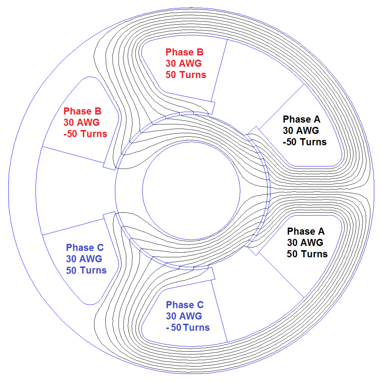
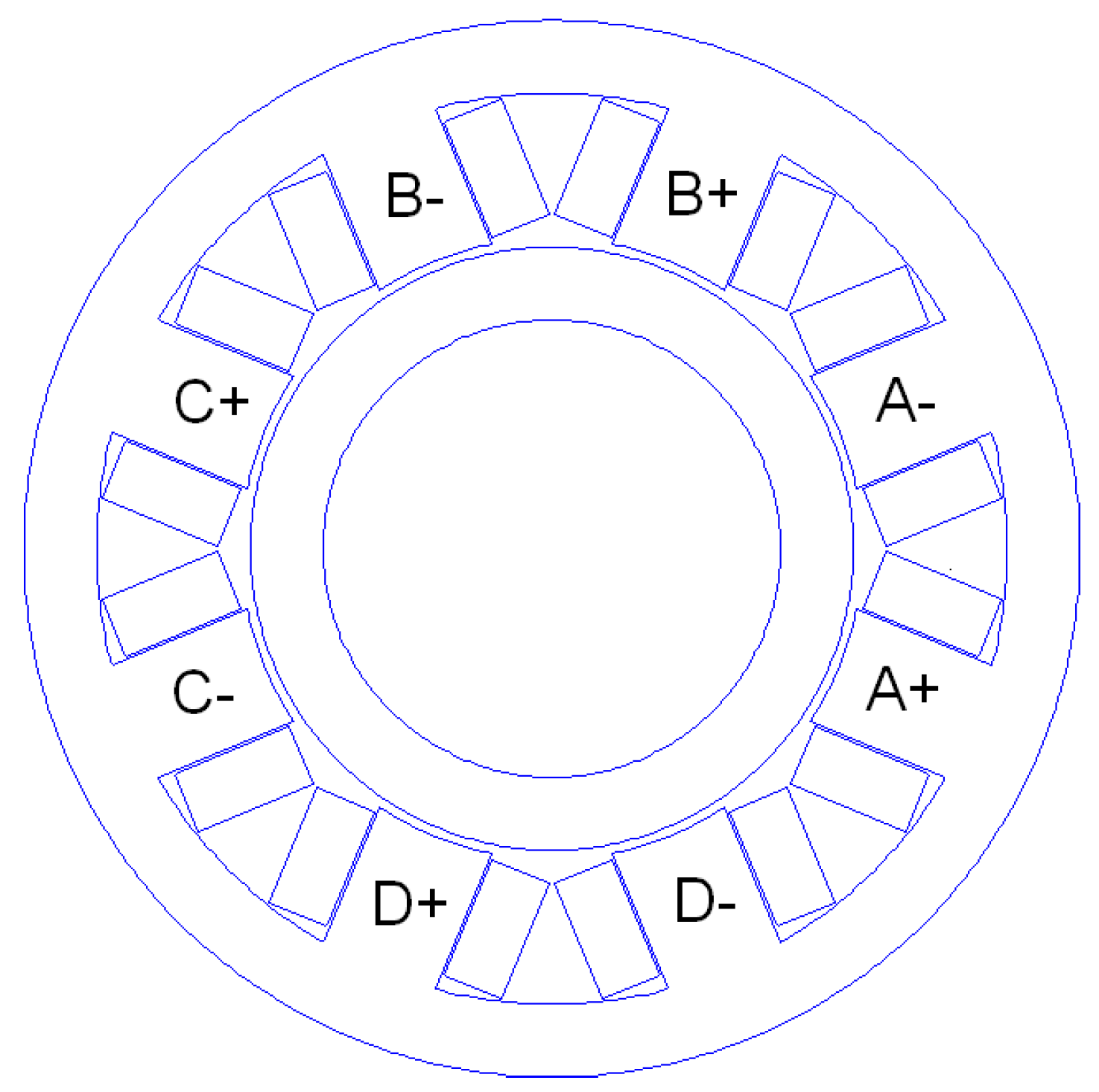
8. Other Practically Important Configurations

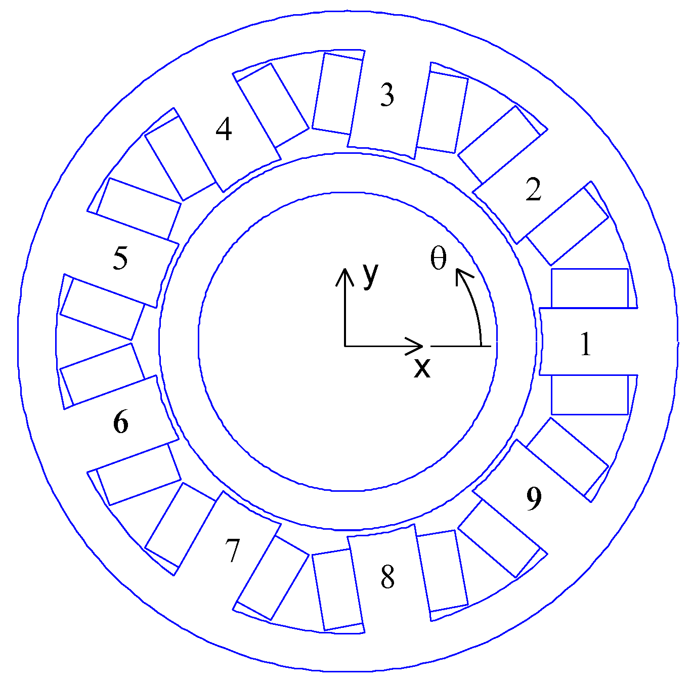
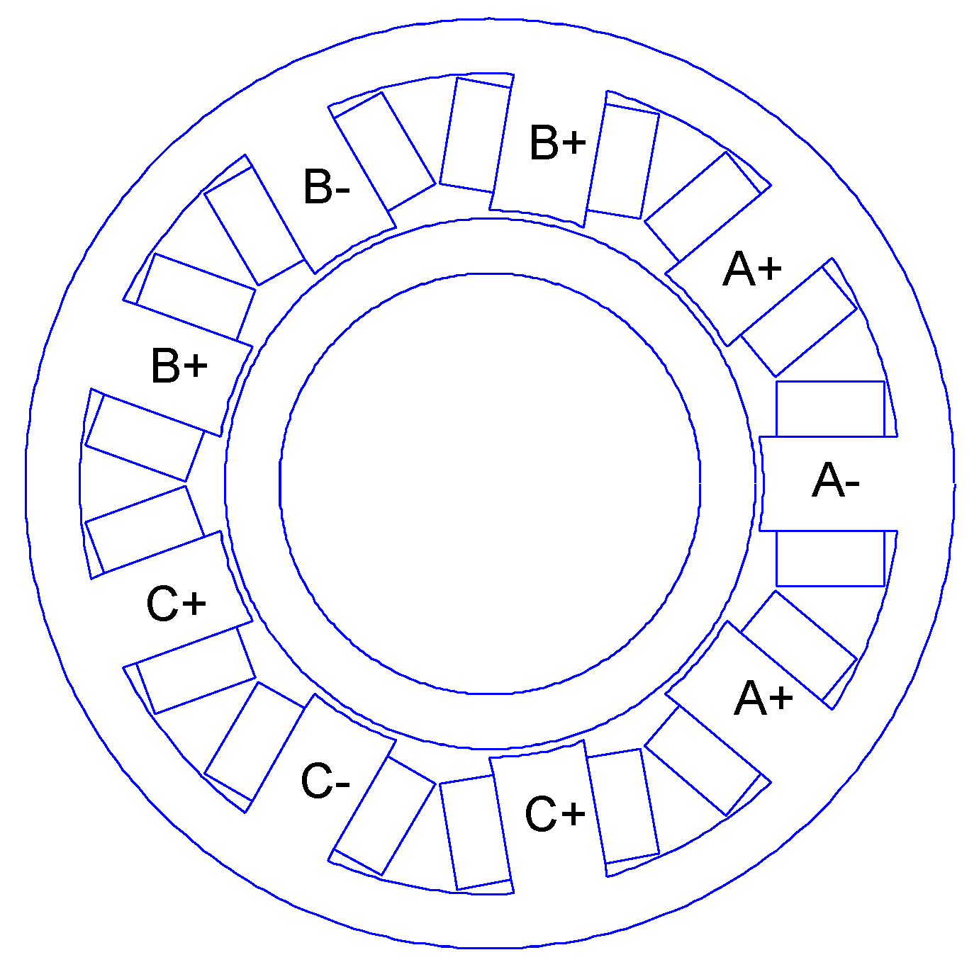
8.1. Nine Pole 3-Phase Bearing

To minimize back iron thickness, a nine-pole bearing might be desired. However, it may also be desirable to reduce the electrical complexity and wire count to the greatest possible degree by driving the bearing with one 3-phase amplifier instead of the 3 × 3 configuration. This situation is addressed by a nine-pole bearing, where each three successive poles are wound in reverse series, as shown below in Figure 3.

In this case, a scaled version of the the Inverse Clarke transformation is again a solution for $\mathit{W}$:

$$\mathit{W}=\left(\begin{array}{cc}1.02623& 0\\ -0.513115& -0.888742\\ -0.513115& 0.888742\end{array}\right)$$

(41)

The required back iron area = $1/\sqrt{3}$ = 0.57735 of the pole area, implying a slightly thicker back iron than would be required by the 3 × 3 phase bearing. Because the currents are not optimally distributed among the poles, the nine-pole 3-phase bearing has a load capacity that is 84.4% of the 3 × 3 configuration.

8.2. Eight-Pole Horseshoe Bearing

The operation of magnetic bearings with zero bias flux has been a subject of several recent works such as [10,11]. These works consider eight-pole horseshoe-type magnetic bearings and treat each axis as a separate one-degree-of-freedom (1-DOF) system. As is shown in [11], the force slew rate is limited near zero force for a 1-DOF bearing operating with zero bias. This slew rate limiting results in cross-over distortion when the force passes through zero on either axis. In contrast, the present approach is a fundamentally 2-DOF unbiased control method. This 2-DOF method is subject to slew rate limiting only when the force is near zero on both axes at the same time. Although the present control technique seems best suited to bearings with an odd number of poles, it also applicable to the common eight-pole bearing wound in a horseshoe configuration. The result is a zero bias control strategy for eight-pole magnetic bearings that is less prone to slew rate limiting than the approaches considered in other recent works.

The horseshoe configuration has N turns around each of the poles that form the horseshoe, and the two poles are connected in reverse-series. This configuration is shown as Figure 4, where A, B, C, and D represent each of the bearing’s four electric circuits.

Each of the four horseshoes is driven with an independent switching amplifier running in closed-loop current control mode. In terms of the four independent currents, the ${\mathcal{X}}_x$ and ${\mathcal{X}}_y$ matrices that relate current to force reduce to diagonal matrices:

$${\mathcal{X}}_x=\left[\begin{array}{cccc}cos\left(\frac{\pi }{8}\right)& 0& 0& 0\\ 0& 0& 0& 0\\ 0& 0& -cos\left(\frac{\pi }{8}\right)& 0\\ 0& 0& 0& 0\end{array}\right]$$

(42)

$${\mathcal{X}}_y=\left[\begin{array}{cccc}0& 0& 0& 0\\ 0& cos\left(\frac{\pi }{8}\right)& 0& 0\\ 0& 0& 0& 0\\ 0& 0& 0& -cos\left(\frac{\pi }{8}\right)\end{array}\right]$$

(43)

With these diagonal matrices, a scheme similar to Equation (32) can then be employed to determine a valid $\mathit{W}$ matrix, where the angles used in Equation (32) are the average angle of each horseshoe and a scaling factor of $1/\sqrt{cos(\pi /n)}$ is used in place of $\sqrt{8/n}$:

$$\mathit{W}=\frac{1}{\sqrt{cos\left(\frac{\pi }{8}\right)}}\left[\begin{array}{cc}1& 0\\ \frac{1}{\sqrt{2}}& \frac{1}{\sqrt{2}}\\ 0& 1\\ -\frac{1}{\sqrt{2}}& \frac{1}{\sqrt{2}}\end{array}\right].$$

(44)

The non-dimensional load capacity with this control approach is $cos\left(\frac{\pi }{8}\right)=0.92388$, and the required back iron fraction is also $0.92388$. The bearing has the same load capacity as a bias-linearized bearing and requires the same back iron thickness as a bias-linearized bearing with an NNSSNNSS biasing scheme. However, the present scheme operates the bearing without bias, reducing the resistive and rotating losses in the bearing.

9. Position Variation

The results to this point have considered the inversion of the current-to-force relationship in the case where the rotor is centered within the bearing. However, the rotor is expected to move within the air gap. In bias-linearized bearings, the effect of position offset is represented by linearizing force about small rotor displacements to obtain a magnetic stiffness. Here, force can also be linearized for small displacements to deduce the position-dependence of the force. On the basis of the derived position-dependence of the force, the commanded currents can be corrected to cancel out the position dependence, resulting in currents that realize the commanded force, regardless of rotor position.

Let X and Y represent rotor displacement non-dimensionalized by nominal gap length, g, in the x- and y-directions, respectively. Equation (6) representing the relationship between current and force can be linearized for small X and Y as

$$f\approx \left\{\begin{array}{cc}{i}_r& i_i\end{array}\right\}{W}^{\prime }\left(\left({\mathcal{X}}_x+X\frac{d{\mathcal{X}}_x}{dX}+Y\frac{d{\mathcal{X}}_x}{dY}\right)+j\left({\mathcal{X}}_y+X\frac{d{\mathcal{X}}_y}{dX}+Y\frac{d{\mathcal{X}}_y}{dY}\right)\right)W\left\{\begin{array}{c}{i}_r\\ i_i\end{array}\right\}.$$

(45)

To frame position variation results in a more compact form, the rotor displacements can be represented by a single complex-valued quantity, d,

$$d=X+jY.$$

(46)

To bring Equation (45) back to a relatively compact complex form, complex representations of X, Y, $i_r$ and $i_i$ can be substituted, i.e.,

$$\begin{array}{ccc}\hfill X& =& (d+\overline{d})/2,\hfill \\ \hfill Y& =& (d-\overline{d})/\left(2j\right),\hfill \\ \hfill i_r& =& (i+\overline{i})/2,\hfill \\ \hfill i_i& =& (i-\overline{i})/\left(2j\right),\hfill \end{array}$$

(47)

where the over-bar notation represents the complex conjugate.

In the general case, Equation (45) does not have a simpler complex form. However, the specific symmetric cases where $\mathit{W}$ is prescribed by Equation (32), Equation (45) does yield simple expressions. For a three-pole bearing, the force linearized about small displacements is

$$f=i^2+di\overline{i}.$$

(48)

For bearings with an odd number of poles greater than three, the dependence of force on position is

$$f=i^2+2di\overline{i}.$$

(49)

A correction to the currents to account for position variations in Equation (49) can be obtained by linearizing the currents about the nominally desired current (i.e., the desired current that is computed for the centered rotor position), denoted here as $i_{des}$. The current can be written in terms of a $i_{des}$ and a perturbation current, $\delta i$ as

$$i=i_{des}+\delta i.$$

(50)

Expanding Equation (49) and neglecting second order terms in $\delta i$ and d results in the expression:

$$f=i_{des}^2+2i_{des}\delta i+2d{i}_{des}{\overline{i}}_{des}$$

(51)

Since current $i_{des}$ is selected to yield the nominally desired force, current $\delta i$ can then be selected to cancel out the last two terms

$$2i_{des}\delta i+2d{i}_{des}{\overline{i}}_{des}=0.$$

(52)

Solving for $\delta i$ yields

$$\delta i=-d{\overline{i}}_{des},$$

(53)

so that the total commanded currents, $i_{cmd}$, that yields the desired force and rejects variations in position, is

$$i_{cmd}=i_{des}-d{\overline{i}}_{des},$$

(54)

where the $i_{des}$ is the square-root of the desired force:

$$i_{des}=\sqrt{f_{des}}$$

(55)

The position dependence of the nine-pole/3-phase bearing and the eight-pole horseshoe bearing considered in Section 8 are also closely approximated by Equation (49), so Equation (54) can be employed to mitigate most of the position dependence in those cases as well.

10. Conclusions

A generalized unbiased control strategy for heteropolar magnetic bearings has been presented. The approach is particularly suited to bearings with an odd number of poles. Depending on the choice of pole count, 3-phase motor drives can be used to control currents in the bearing, thereby reducing hardware complexity, cost, and wire count. As noted in [1], the scheme is relatively immune to slew rate limiting. Slew rate limiting is only possible when both components of force are near zero simultaneously.

The scheme also allows for fault-tolerant operation. In the most general realization, each pole is driven by an independently controlled amplifier. However, it is alternatively possible to have redundant sets of 3-phase drives rather than single phase drives. Current mappings ($\mathit{W}$ matrices) that control the bearing in every possible fault configuration are numerically computed offline, a one-time computation performed during the design of the controller. If a fault occurs, the controller switches over to a precomputed current mapping that matches the faulted configuration. The realization of this method of fault tolerance would be very similar to that experimentally demonstrated in [9], where a set of $\mathit{W}$ matrices that solve the closely related generalized bias linearization problem for each faulted configuration are precomputed and used as needed if faults occur.

There are many other possible extensions of the present work. Specifically, the performance of the scheme could be experimentally investigated. Interesting possibilities include the experimental realization of the nine-pole 3-phase or 3 × 3 bearings or a comparison of the performance of the eight-pole horseshoe strategy to the 1-DOF zero bias control strategy. Alternatively, the scheme could be extended to consider actuators with more than two degrees of freedom by seeking a form of the current-to-force relationship described by hypercomplex numbers rather than complex numbers.

References

1. Meeker, D.C.; Maslen, E.H. Analysis and control of a three pole radial magnetic bearing. In Proceedings of the Tenth International Symposium on Magnetic Bearings, Martigny, Switzerland, 21–23 August 2006.
2. Vadillo, J.; Echeverria, J.M.; Elosegui, I.; Fontan, L. An approach to a three-pole active magnetic bearing system fed by a matrix converter. In Proceedings of the Eleventh International Symposium on Magnetic Bearings, Nara, Japan, 26–29 August 2008.
3. Beizama, A.M.; Echeverria, J.M.; Martinez-Iturralde, M.; Egana, I.; Fontan, L. Comparison between pole-placement control and sliding mode control for three-pole radial magnetic bearings. In Proceedings of the International Symposium on Power Electronics, Electric Drives, Automation, and Motion (SPEEDAM 2008), Ischia, Italy, 11–13 June 2008.
4. Matsuda, K.; Kijimoto, S. An approach to designing a magnetic-baring system for smaller rotating machines. In Proceedings of the IEEE International Symposium on Industrial Electronics, Cambridge, UK, 30 June–2 July 2008.
5. Maslen, E.H.; Meeker, D.C. Fault tolerance of magnetic bearings by generalized bias current linearization. IEEE Trans. Magn. 1995, 31, 2304–2314. [Google Scholar] [CrossRef]
6. Popescu, M. Induction Motor Modelling for Vector Control Purposes; Helsinki University of Technology: Espoo, Finland, 2000. [Google Scholar]
7. Na, U.J.; Palazzolo, A. Optimized realization of fault-tolerant heteropolar magnetic bearings. J. Vib. Acoust. 2000, 122, 209–221. [Google Scholar] [CrossRef]
8. Boyd, S. Least-Norm Solutions of Underdetermined Equations. Available online: https://see.stanford.edu/materials/lsoeldsee263/08-min-norm.pdf (accessed on 6 November 2016).
9. Maslen, E.H.; Sortore, C.K.; Gillies, G.T.; Williams, R.D.; Fedigan, S.J.; Aimone, R.J. Fault tolerant magnetic bearings. Trans. ASME 1999, 121, 504–508. [Google Scholar] [CrossRef]
10. Jastrzebski, R.P.; Smirnov, A.; Mystkowski, A.; Pyrhönen, O. Cascaded position-flux controller for AMB system operating at zero bias. Energies 2014, 7, 3561–3575. [Google Scholar] [CrossRef]
11. Mystkowski, A.; Pawluszewicz, E.; Dragašius, E. Robust nonlinear position-flux zero-bias control for uncertain AMB system. Int. J. Control 2015, 88, 619–1629. [Google Scholar] [CrossRef]
Figure 1. Small three-pole bearing with 0.25 inch rotor outer diameter.
Actuators 06 00001 g001
Figure 2. Nine-pole bearing showing pole orientation.
Actuators 06 00001 g002
Figure 3. Nine-pole 3-phase bearing with a [A,−A,A,B,−B,B,C,−C,C] winding.
Actuators 06 00001 g003
Figure 4. Eight-pole magnetic bearing with a horseshoe winding.
Actuators 06 00001 g004