1. Introduction
Conventional AMBs (active magnetic bearings) [
1,
2,
3], here called Type A, are based on the structure shown in
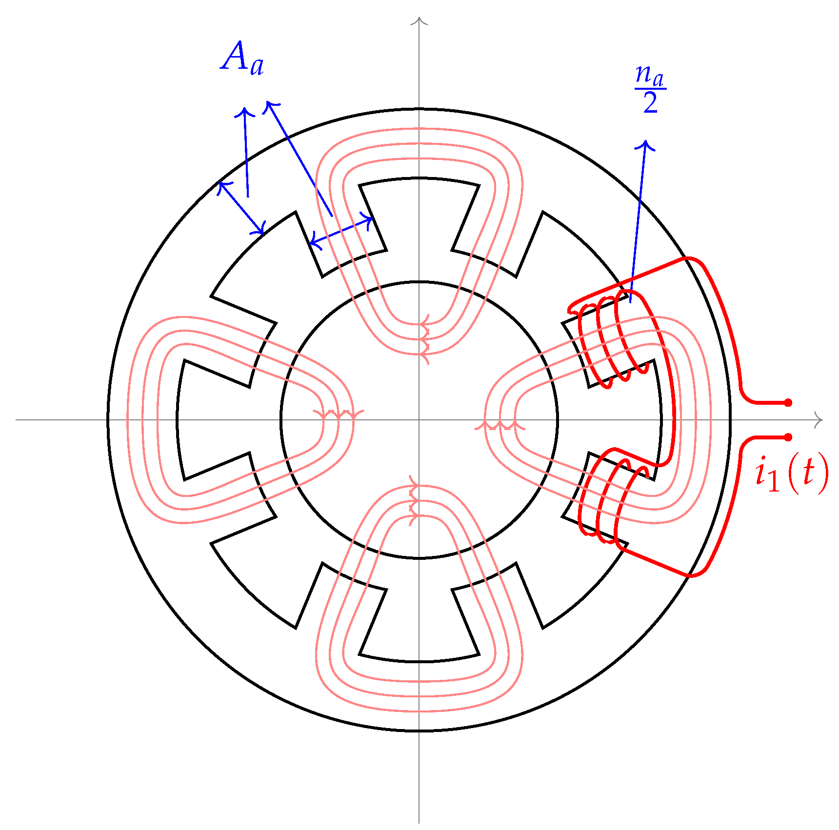
Figure 1. There are four “U-shaped electromagnets”, two for the
x or horizontal direction and two in the
y or vertical direction, resulting in four independent magnetic flux loops.
The windings in the
x and
y direction are fed with currents
and
; the constant current
is the base, or bias, and the differential currents
and
will control the rotor position. Using basic reluctance concepts, the resultant forces
and
can be expressed in terms of these currents, the air magnetic permeability
, the total number of coils
, the cross-section area in the stator ferromagnetic material
and the nominal length
h of the air gaps. After a standard linearization procedure [
1] around the operating point
, the forces generated by the Type A structure are shown in (
1). Notice that the unconnected nature of the magnetic fluxes leads to uncoupled forces:
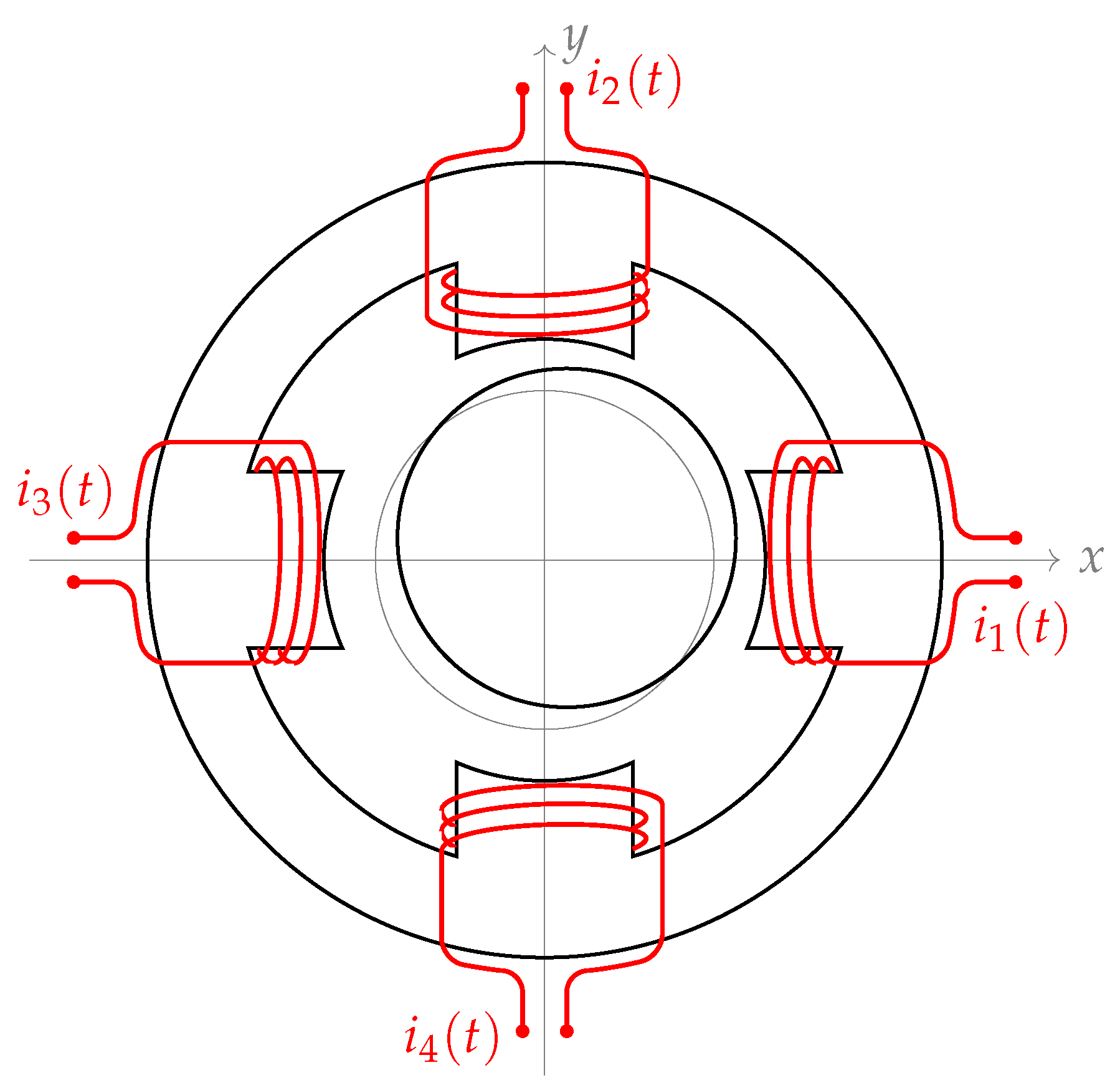
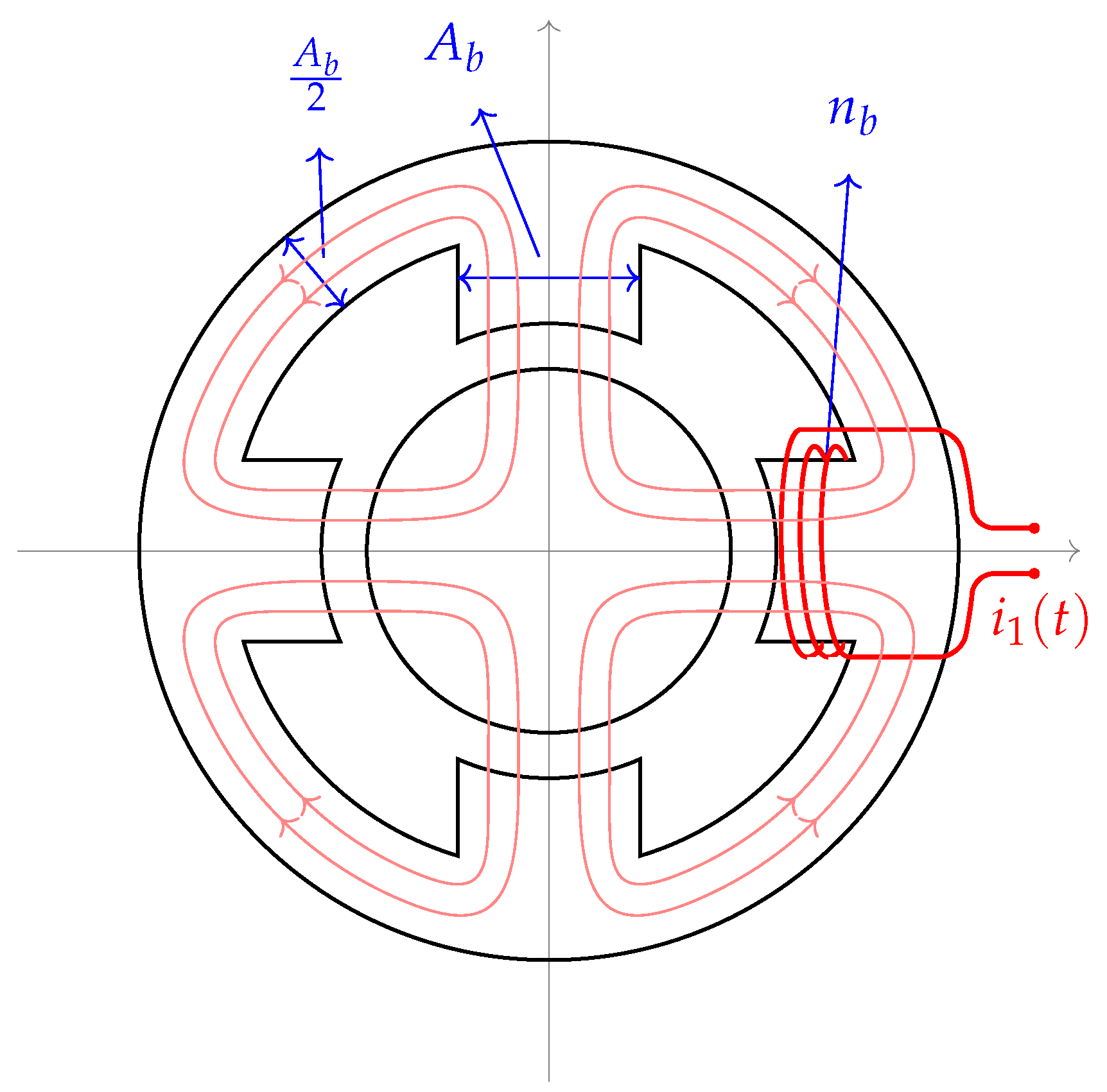
A different structure for magnetic bearings, here named Type B, is possible, with four windings that lead to interconnected magnetic loops, as depicted in
Figure 2. This structure is found in the split-winding self-bearing motors researched in Brazil [
4,
5,
6,
7,
8,
9,
10], among others. In that approach, to provide a simultaneous torque, alternate currents are injected into the windings; for AMBs, DC currents are considered.
It is now appropriate to discuss, in a preliminary way, some aspects of this different geometry for AMBs. At first glance, it seems safe to state that Type B, with its four- “pole” stator structure, shows a cleaner and more compact design than Type A, which will probably result in more cost-effective manufacturing situations. It is also easy to accept that Type B offers more space for heat dissipation and that the flux losses in its coils are smaller.
It is clear that all of the very desirable Type B characteristics in the above paragraph do not represent true facts yet: they are only very reasonable conjectures that must be thoroughly tested before definite conclusions can be made. If all of these considerations turn out to be true, then the Type B geometry must be seen as a valid alternative to, if not as a better choice than, Type A for AMBs.
The main goal of this work is to discuss at some depth yet another aspect of this “reduced pole” geometry: its capability of generating restoring forces
and
that are potentially better for AMBs than those in the eight-“pole” case. It will be shown, in a theoretical way, that the linearized restoring forces for Type B are similar to those for Type A, shown in (
1), but with a higher magnitude. Is this ability of generating higher forces a desired characteristic for AMBs? This problem will also be addressed in this paper, with the help of examples. In order to assure that the theoretical conclusions for the four-pole geometry hold true in the real world, a series of laboratory tests is necessary. The final sections in this article deal with prototypes that have been built for Types A and B and consider the possible tests capable of comparing the force-generating performances of both structures.
This paper is based on ongoing research [
11,
12,
13]. Its first stage, shown here, is based on theoretical considerations and on simulations; the last steps of this research, the important laboratory tests that can validate all of the initial considerations, are not ready yet, and will be presented in a future work. The material covered in this article is spread throughout the sections as follows. A mathematical model, based on elementary reluctance concepts, is detailed in
Section 2, which tracks closely [
11] and [
12]. This model explains the generation of reluctance forces
and
in Type B bearings; the linearized final expressions for these forces show a decoupled nature, similar to those for Type A in (
1). In addition, the position and current constants,
and
, are shown to have higher values than in the A case.
Section 3 presents analytical results and simulations on how increased values of
affect the dynamics and control aspects of AMBs in a positive way [
12]; simple examples that illustrate meaningful control situations are used. The prototypes built to the laboratory tests that will compare Types A and B are shown in
Section 4; a mathematical model describing their dynamic behavior is developed. In
Section 5, simulations of some control laws applied to the prototypes are made, and their results are discussed. The importance of this section is that the control laws used here will be the ones driving the prototypes in the real tests. Discussions about the future real tests, final comments and general considerations on what remains to be done are made in
Section 6.
Other results are known in the literature with the Type B bearing concept. In [
14], a Type B structure is used to minimize rotor vibrations; a non-linear expression for the bearing forces is mentioned by the authors. The Type B geometry is used in a magnetic force determination problem, in [
15]; some steps are taken toward a reluctance model for the bearing forces. A patent for a Type B bearing was claimed and granted in [
16], where some superior aspects of this structure are described. This short list is all that the authors could find.
None of the references above shows a detailed mathematical model, neither nonlinear nor linear, for the reluctance forces generated in a Type B structure, or any type of comparisons with Type A, like the ones presented in the next sections. The main contribution of this work is this mathematical model and the comparisons between the two possible types of AMBs.
2. Force Generation in Type B Bearings
A detailed study of the force generation in the flux interconnected structure (Type B) was presented in [
6,
11,
12]; the main points are now repeated. The
x and
y components of a radial displacement of the rotor change the nominal gap width
h, as shown in
Figure 3.
To compensate the displacements, it is usual to apply differential currents [
1] to the pairs of windings: the differential, or control, currents
, for the
x or horizontal direction, and
, for the vertical direction, are added and subtracted to a base, or bias, current
, a constant DC level. The total currents imposed at each winding are:
Light pink lines in
Figure 2 represent the magnetic flux distribution caused by these currents. The reluctance forces depend on the magnetic fluxes
, in the four air gaps with cross-section
:
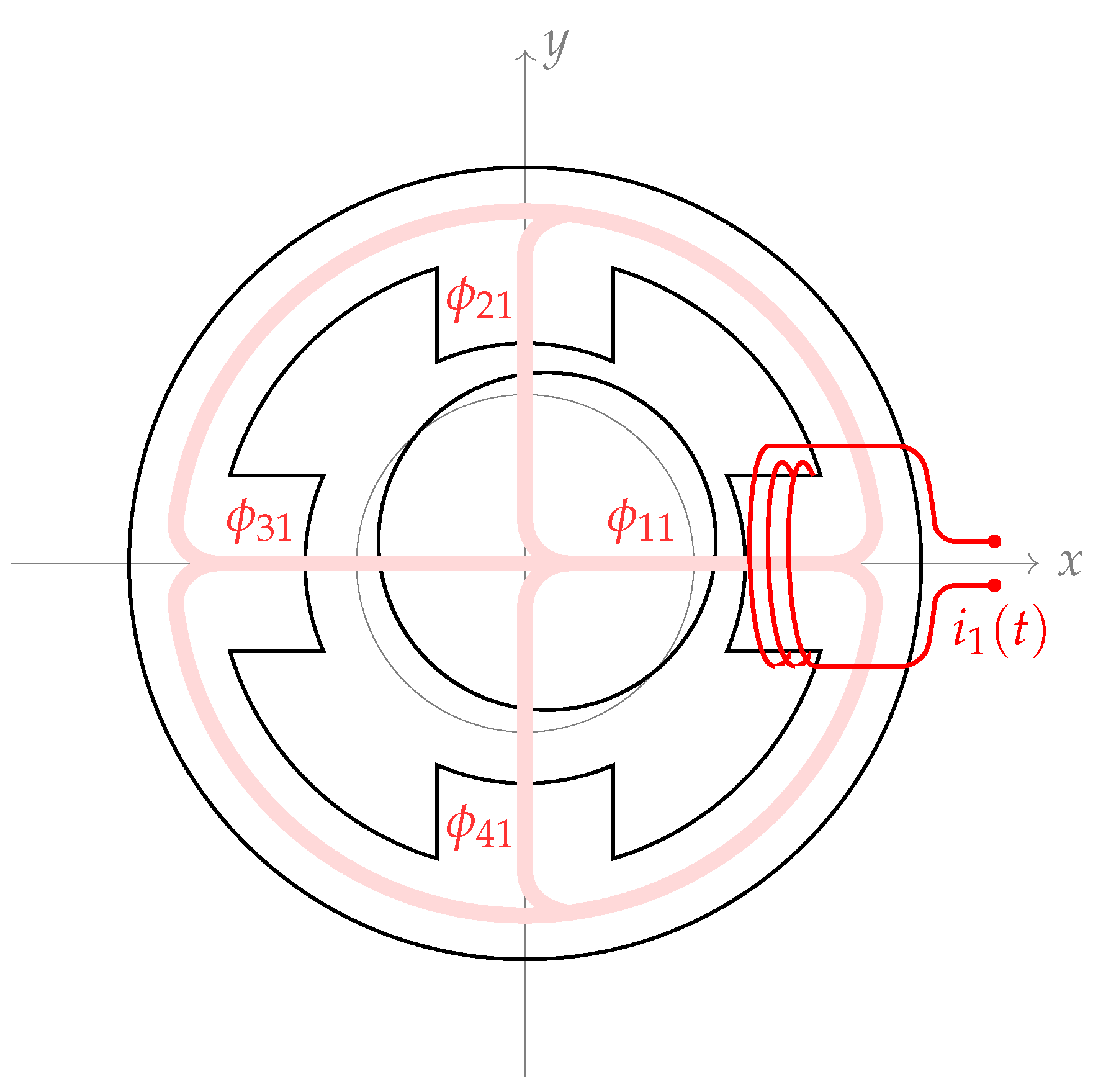
The ferromagnetic connections in Type B allow a current injected in any winding to cause fluxes in all four air gaps;
Figure 4 illustrates the effects of
in all four “poles”. If
denotes the flux in air gap
j caused by a current in winding
k, the total magnetic flux
in “Pole” 1 is a function of the fluxes
. Assuming no air or ferromagnetic losses and positive signs for fluxes headed to the rotating center, the total magnetic fluxes in the poles are:
For the determination of the
, let the magneto-motive force generated by
be denoted by
and the reluctance of the air gaps in the four poles in
Figure 3 by
,
,
and
. Recalling that
is the cross-section area of the poles in
Figure 2 and that the displacements
h,
x and
y are explained in
Figure 3, the reluctances are expressed by:
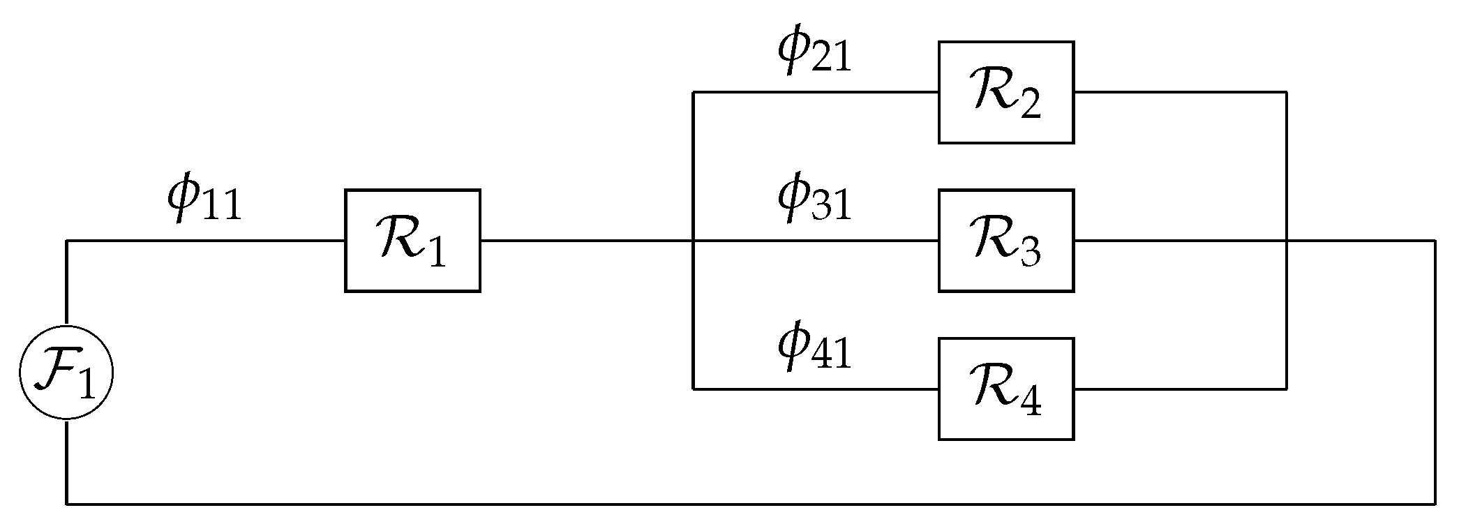
The equivalent circuit that models the magnetic flux situation in a Type B structure is shown in
Figure 5.
A simple way to extract information from magnetic circuits like the one in
Figure 5 is by using the passive electric circuit analogy: fluxes are treated as currents; operations with reluctances are the same as those with resistances; and the usual operations allowed in Kirchoff’s rules are valid. It is easy to see that in the circuit under study, reluctance
is in series with the parallel combination of reluctance
,
and
. If
denotes the equivalent reluctance of the parallel combination:
that easily leads to the value of
. Therefore, the magnetic circuit in
Figure 5 can be replaced by a single reluctance
given by:
and, finally:
To avoid cumbersome formulas, some auxiliary variables are defined:
Since
, algebraic operations lead to expressions for the fluxes associated with
imposed on the winding in Pole 1 of
Figure 3:
The same procedure, repeated for currents
,
,
imposed at the windings in Poles 2, 3 and 4 in
Figure 3 results in:
The total fluxes
for
can be determined by substituting the previous values of the partial fluxes
in Equations (
5) and (
6). Then, with the help of (
4), the total reluctance forces generated in a Type B magnetic bearing can be expressed as:
where
are complicated functions of their arguments:
with
The currents
are defined in Equations (
2) and (
3); if the distances
and
are denoted by
and
, the
above are:
The complexity of the above formulas makes the linearization of (
16) a hard task. Considering that the AMB operates around a point
, the use of symbolical computation, or even a pen on paper procedure, allows the calculation of the partial derivatives:
If a similar procedure is made for
, the combined results lead to the linear expressions for the Type B structure forces:
Two remarkable aspects are to be noted when these expressions are compared with the ones in (
1): (a) even though the fluxes are interconnected in a Type B structure, the forces are decoupled, exactly as they were in Type A; (b) a factor of two appears in the formulas above for the
, which was not present in Case A.
In the above developments, an underlying assumption is made: there is no magnetic saturation. What happens when both types are saturated? This is a pertinent question that cannot be answered with theoretical tools: extensive laboratory tests would have to be done.
3. Theoretical Comparisons
Assuming the same outside diameter of the stator, the following characteristics can be identified for the Type B active magnetic bearing when it is compared with Type A:
- (1)
The position and current constants
and
in (
20) are two-times bigger than their counterparts
and
in Equation (
1);
- (2)
the cross-section area can be chosen greater than ; it is reasonable to have ;
- (3)
the number of coils can, possibly, be larger than .
The net conclusion is: the position () and current () constants for Type B AMBs have values at least two-times higher than in Case A. Depending on the design aspects ( and ), even higher rates can be achieved. How much can these constants be increased? The magnetic saturation seems to be the limit. Higher valued coefficients mean, at first sight, higher forces for the same input currents and displacements and a different dynamic behavior for Type B. Are these effects beneficial in the AMB performance? Are they sound advantages?
To evaluate the effects of
and
in an AMB operation, a theoretical analysis was applied, in [
12], to a simple, but meaningful, control problem, where many aspects of the real-life functioning of AMBs are present. That material is summarized in
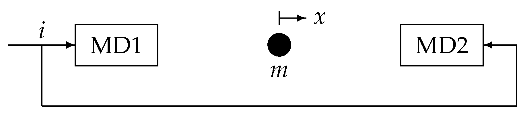
Figure 6: a particle moving without friction in a horizontal, rectilinear path is to be positioned.
The magnetic devices MD1 and MD2 apply a resultant force
on the sphere, where
i is a control current and
x is the displacement. A controller is desired, for driving
x(
t) to zero for all possible initial conditions, and in the eventual presence of constant, horizontal disturbance forces
d. A mathematical model can be found with a simple application of Newton’s law:
. The linear nature of
f leads to
, which can be expressed, with the use of Laplace transforms, as
. The particle position (its Laplace transform) is, therefore, given by:
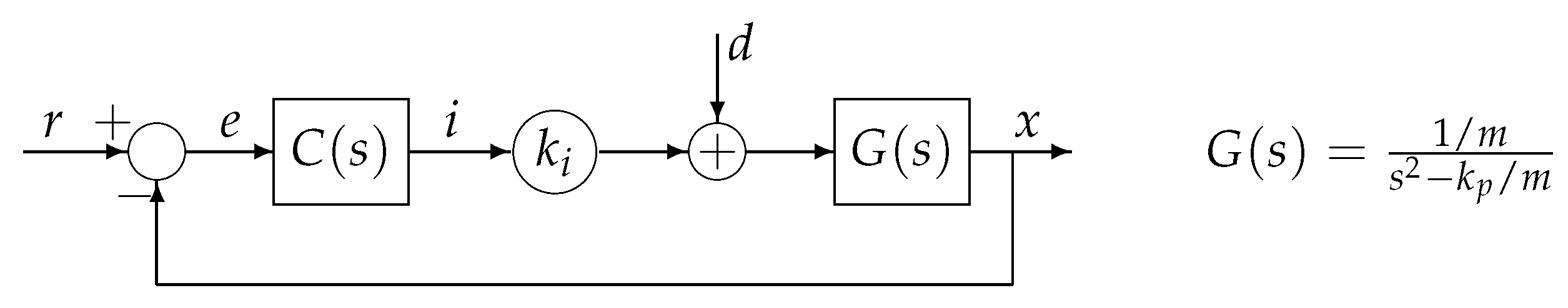
where
G(
s) is called the plant transfer function. The controller’s output is the current
i and its input is the error signal
where
r is an external reference that indicates the desired behavior of
x (in this case,
). If
is the controller transfer function, then, using the Laplace transforms:
Combining (
21) and (
22), it is possible, after some direct algebraic manipulations, to see how the overall output
x depends on the command input
r and the disturbance input
d:
The command transfer function
measures the effect of the reference input
r on the closed loop behavior; it is common to say that controllers are designed to make
as close to unity as possible, meaning that
x must be as close to
r as possible. The disturbance transfer function
indicates how the controlled output
x depends on
d; controllers should, ideally, make
as close to zero as possible. Block diagrams, widely used in control studies, are a very convenient tool for presenting expressions like (
21) and (
22) in an easy to understand graphical way. The block diagram in
Figure 7 models the use of a controller
in the particle problem.
It is possible, using the simple rules of the so-called block diagrams algebra, to extract
and
from block diagrams, which is easier and faster than the above manipulations leading to (
23). These last paragraphs cover basic control aspects and can be found in almost all textbooks on the field.
A stabilizing PD controller
guarantees that initial displacements
are corrected, when
. The speed of convergence depends on the closed loop poles, which are functions of
α and
β. The effects of extra horizontal forces
d on
x(
t) can be evaluated by
, where
is the disturbance transfer function. For this problem, the effect of
d on
x is described, with the results in (
23) and using
for the PD controller, by:
where the characteristic polynomial coefficients are:
and:
. The steady state influence of disturbances, when
, is measured by
. Assuming closed loop stability, an important property of the Laplace transforms (the final value theorem) says that:
For constant disturbances
this leads to
The well-known fact that PD controllers do not completely reject (
) constant disturbances becomes apparent. However, Equation (
24) tells more: for a fixed, stabilizing controller,
decreases when
and
increase by the same factor. In other words, if the position and current coefficients in a magnetic force generation law are both increased by the same amount, the resulting PD control is less sensitive to constant disturbances, and this characterizes a better, stiffer suspension.
Since a full steady state rejection of constant disturbances can be achieved by PID controllers, consider now
. The new disturbance transfer function
is:
Because each coefficient depends on a single controller parameter, the closed loop poles can be arbitrarily assigned. A simple calculation shows that complete rejection () of step disturbances is indeed achieved by the PID controller.
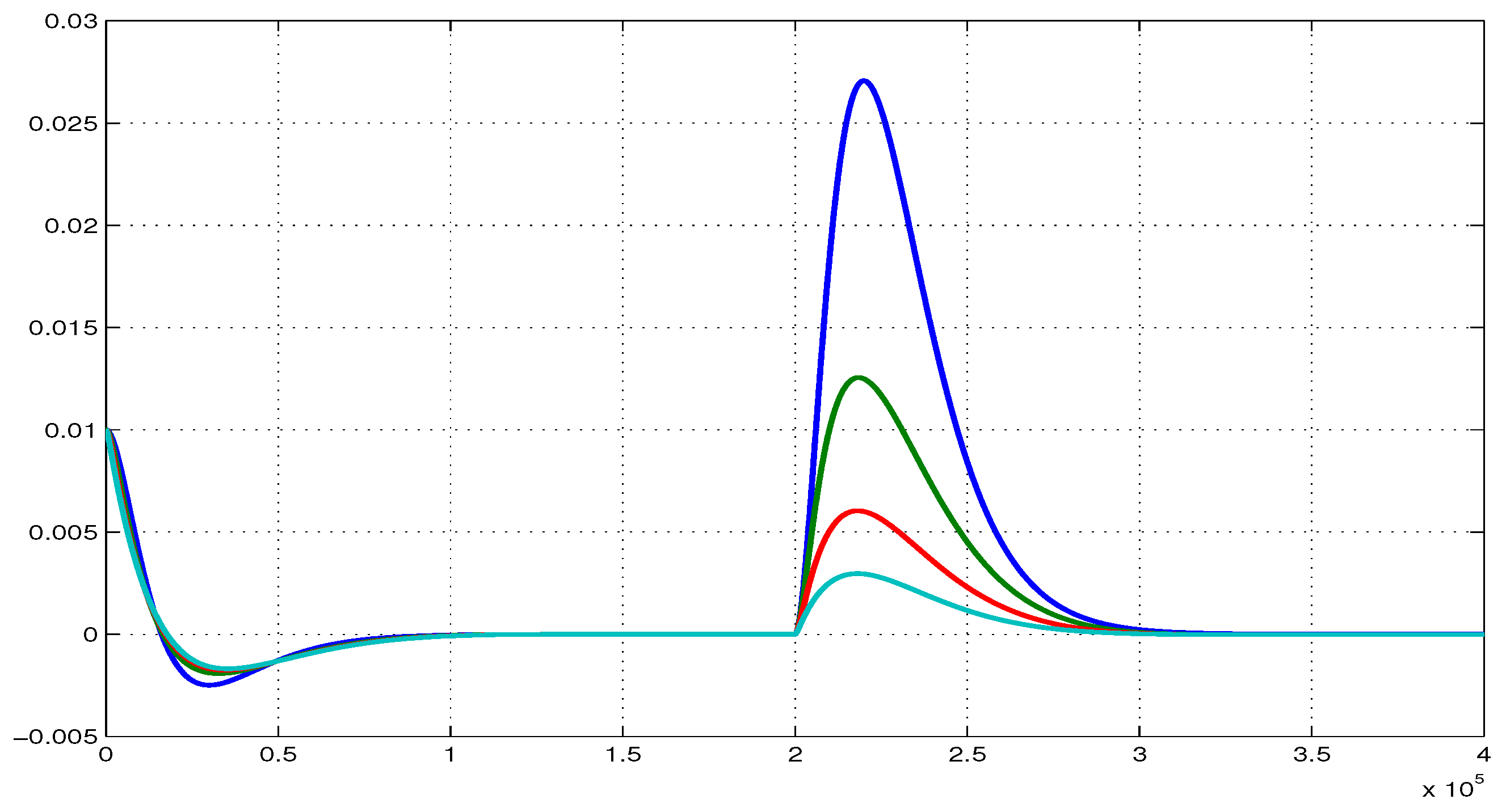
In order to feel the performance details of the situation, a simulation was performed. The numerical values, in the SI system,
,
and
200,000 were used. A PID controller that assigns all of the closed loop poles at
was calculated:
,
= 10,006 and
. An initial displacement of 1 cm was imposed on the sphere, and in less than 1 s, it returned to the desired rest position
. After stabilization, a constant disturbance (
N) was applied and successfully rejected.
Figure 8 shows the curves for different values of the
and
constants:
,
,
and
.
All curves are very similar in the first 2 s, implying that high or low values for the magnetic constants are not crucial in the stabilizing stage. However, when constant disturbance rejection is needed, better transient behaviors are a direct consequence of higher values in and .
The conclusions of this simple example in [
12] are valid in much more general situations, involving real-world applications of practical interest. Additionally, these conclusions are: increasing the values of the magnetic force constants
and
is a highly desirable goal in the AMB field.
4. Prototype Building and Models
The final conclusions of
Section 2 and
Section 3 are that the interconnected fluxes in the Type B structure increase the values of the magnetic force constants
and
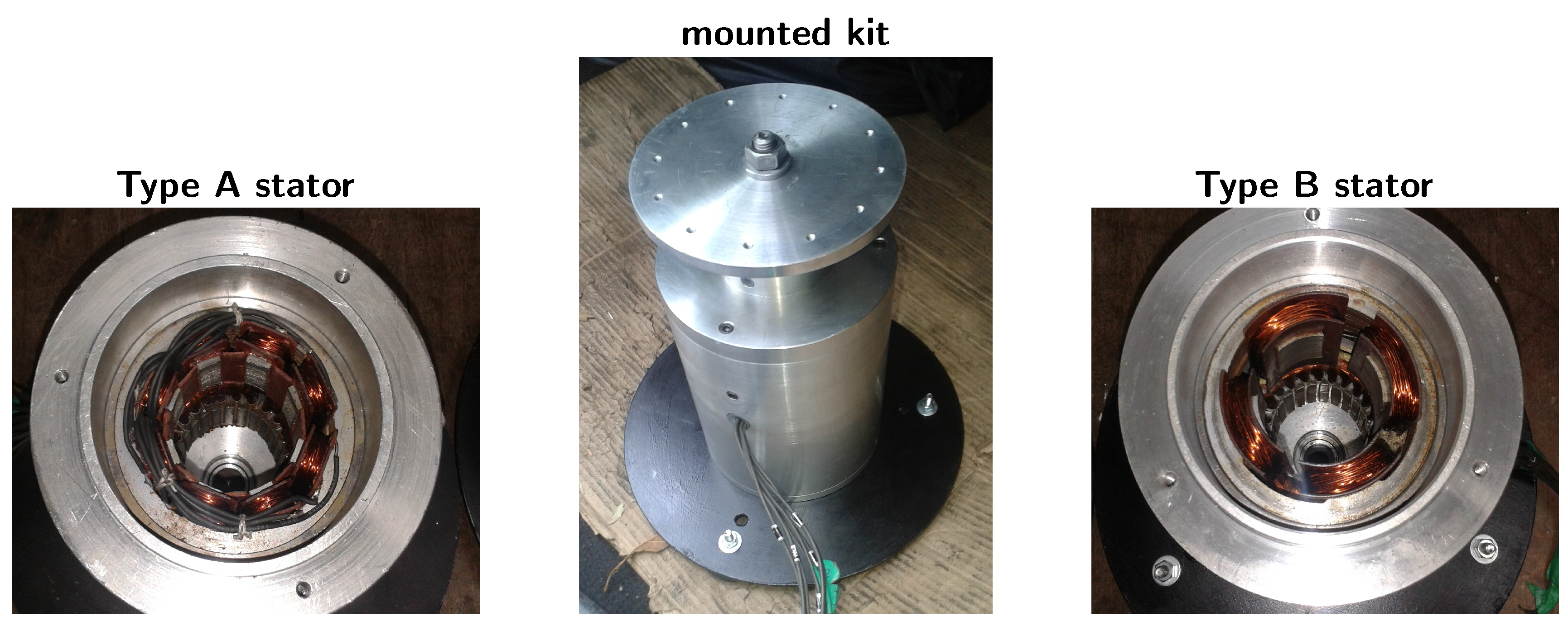
. How sure can one be about the theoretical tools used in those developments? The best possible way to answer this question is by constructing and testing prototypes in an exhaustive way. Only after this stage will the ideas proposed here be validated; or not. Two prototypes, one for Type A and the other for Type B, have been constructed;
Figure 9 shows a top view of them. A vertical rotor with a large, perforated upper disk will fill the above pieces; the same
Figure 9, in the center, shows a view of a mounted kit, with the rotor inserted in the carcass with the stators. The upper disk’s sole purpose is to determine whether Type B is really a stiffer AMB than Type A; see
Section 5. This is because it can generate, in an easy way, as explained in
Section 4.4, harmonic disturbances.
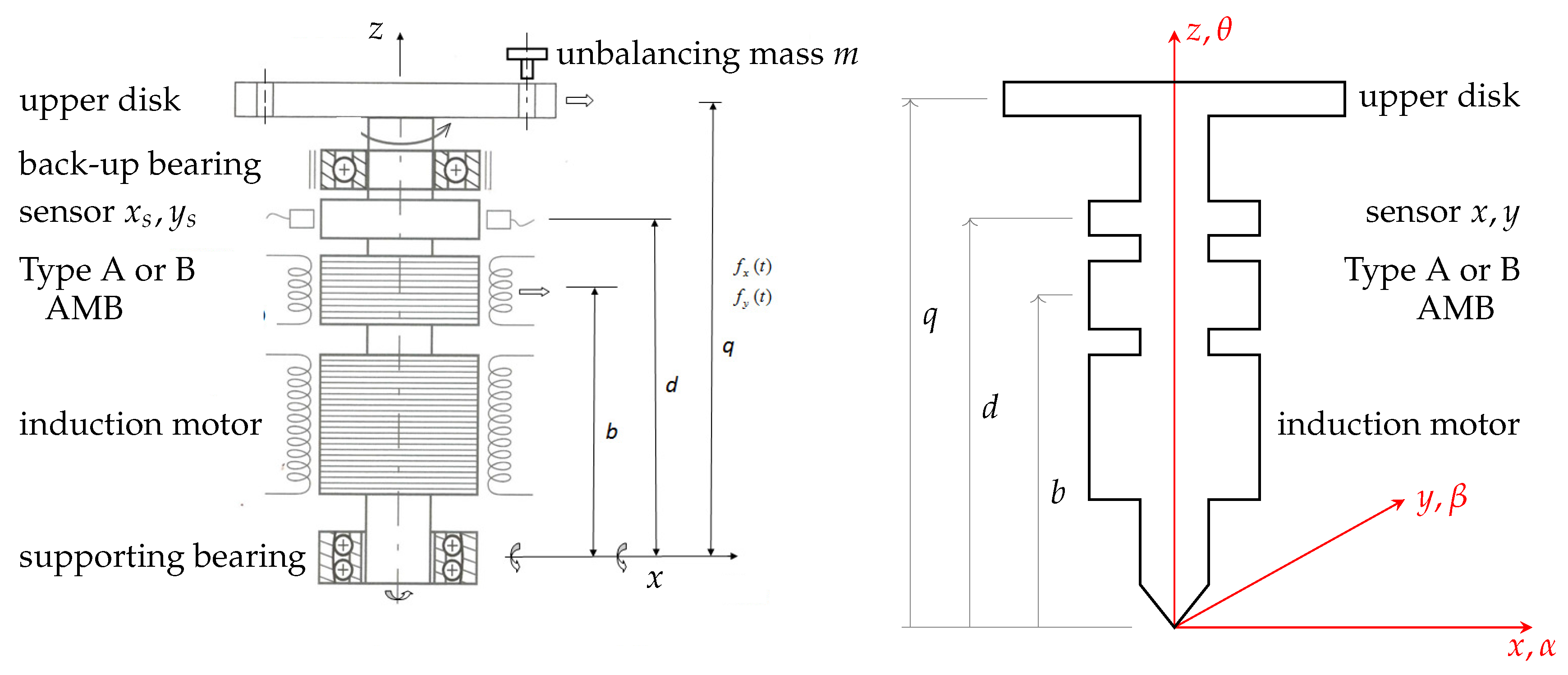
The details of the vertical part are depicted in
Figure 10. The bottom part is a mechanical bearing to prevent vertical movements; just above it there is the rotor of a two-phase induction motor for spinning the shaft. Next comes the AMB rotor, the same for Types A and B, and the sensors’ target. A disk with holes perforated near its edge lies on the upper part.
Traditional procedures, like those in [
1,
3] and Chapter 4 in [
2], will be used to find mathematical models for the prototypes. The self-aligning, supporting bearing at the bottom, while allowing angular movements in any direction, provides a fixed point for the rotor. An inertial reference system is placed at this location; axes
x and
y lie in the horizontal plane, and
z marks the vertical direction. The positive angles
α,
β and
θ can be found by using the right-hand rule on
x,
y and
z. The right half of
Figure 10 sketches the situation; the supporting and back-up bearings are not shown.
Assuming a rigid and homogeneous rotor, the center of mass displacements can be determined by the angles
α and
β, and a full dynamic model can be obtained from the rotational equations alone. Denoting the angular moments of inertia around the three axes by
and
, symmetry considerations assure that
. In the classical Newton–Lagrange framework, the dynamic equations for rotations are:
where
is the rotor angular velocity and
express all external actions generating torques. The main equations above can be displayed in a vector form:
Defining the angular position vector
p and the external excitation vector
E as:
the rotor dynamics is described by:
where
J is the inertia coefficient (or the inertia matrix
) and
G is the gyroscopic matrix:
External torques may come from many different sources, four of which are considered in this paper: the magnetic (
), gravitational (
), supporting bearing (
) and disturbance or mass unbalance (
) torques.
4.1. Magnetic Excitation
Considering
and
the rotor displacements at the AMB position, the forces generated in each direction are:
where the differential currents
and
were discussed in
Section 1, and the coefficients
can refer to either Type A or B. Assuming rigidity and small angular displacements:
which lead to
and
. Equation (
32) becomes:
These forces cause torques
and
. Assuming, again, rigidity and small angular displacements:
and
, which lead to
and
. These magnetic torques can be expanded as:
If
is the magnetic external excitation vector and
is the external input or control vector, a concise expression can be written:
4.2. Gravitational Excitation
Since
α and
β are small angles, the torques caused by the rotor weight acting at its center of mass are negligible:
This is usually the case with vertical rotors; for horizontal ones, gravity must be considered.
4.3. Supporting Bearing Excitation
The supporting bearing has a viscous damper effect; if
is the viscous constant, the torques are modeled by
and
, and the external excitation contribution is:
4.4. Mass Unbalance Excitation
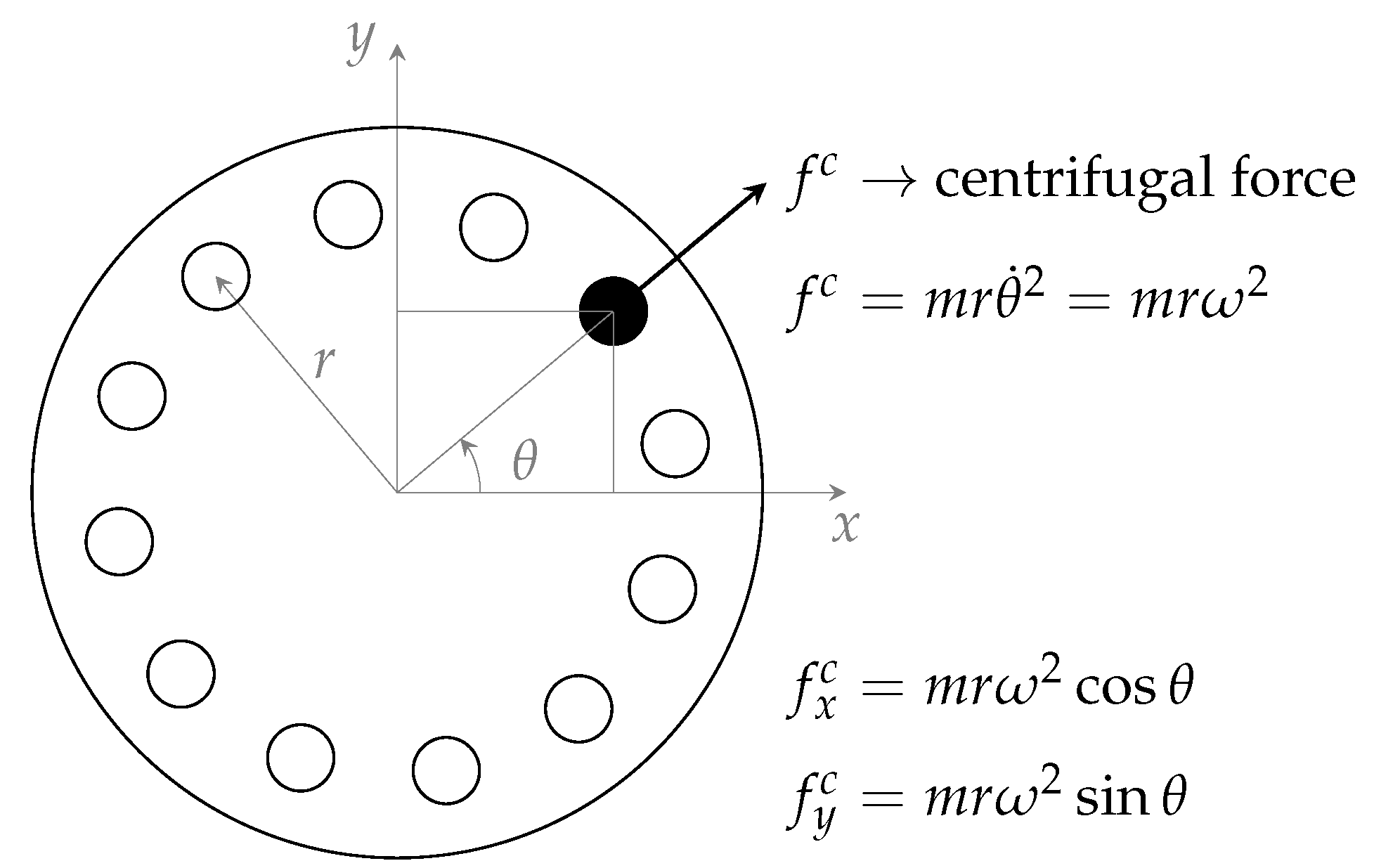
Rotors with a homogeneous mass distribution are assumed in the mathematical model. When, and if, this is not true, unexpected torques appear, acting as disturbances. If these actions are not considered when designing control laws, their effects, sometimes, can be unpleasant and even unacceptable. The upper disk in the considered rotor has 12 holes near the outer edge, placed in a symmetrical way, to preserve the body homogeneity. A small mass
m in one of the holes, as shown in
Figure 11, will act on the rotor with a centrifugal force
, causing an intentional disturbance.
The projections of the centrifugal force on the
x and
y directions are:
and
Since
, the disturbance torques generated by the unbalanced mass are:
and
The mass unbalance external excitation contribution is
where:
are, respectively, the disturbance coefficient and the disturbance input vector.
4.5. Detailed Dynamic Equations
Entering Expressions (
33)–(
36) in Equation (
29) leads, after rearranging terms, to:
It is convenient to rewrite this equation in terms of
and
, the positions measured by the sensors. Rotor rigidity, small angles and geometry considerations guarantee that:
which leads to
and
. If the sensor measurements vector is denoted by
, then:
Multiplying (
38) by
d from the left, using (
39) and dividing by
J, we reach an expression in terms of the sensor positions:
where the parameters are:
In order to express the system dynamic behavior in the state space, the state variables:
can be chosen; Equation (
40) becomes:
where
x,
u and
v have been previously defined,
A is a
matrix and
are
matrices structured as:
where the
blocks are:
It is important to notice that Equation (
42) models a linear system that is time invariant only for a fixed rotational speed, because
depends on
.
5. Prototype Simulations
The simulations in this section do not cover the normal operation of AMBs; they deal with situations where the Case A and B performances have significant differences that can be easily detected in the future laboratory tests. The prototypes’ characteristics were measured, in the SI system; the geometric dimensions are
; the inertia and viscous values are
. A base current
was considered, leading to the magnetic coefficients
207,738,
for Type A and four-times those values for Type B:
830,952,
(SI units). Assuming a constant angular velocity
rpm, corresponding to 356 rad/s, the state space parameters
and
D were calculated for Types A and B, generating matrices
, etc. The open-loop behavior of both types is described by the eigenvalues of the system matrices, listed in
Table 1, and is clearly unstable.
A linear quadratic regulator (LQR) control law was used to stabilize the prototypes. The same performance defining parameters were used for both cases: identity matrices
and
. The resulting gain matrices:
are to be used in the state feedback control laws
. The numerical values in the matrices above are close, meaning that the control efforts can be considered similar in Cases A and B. The closed-loop dynamic behavior can be described by the eigenvalues of
, listed in
Table 2.
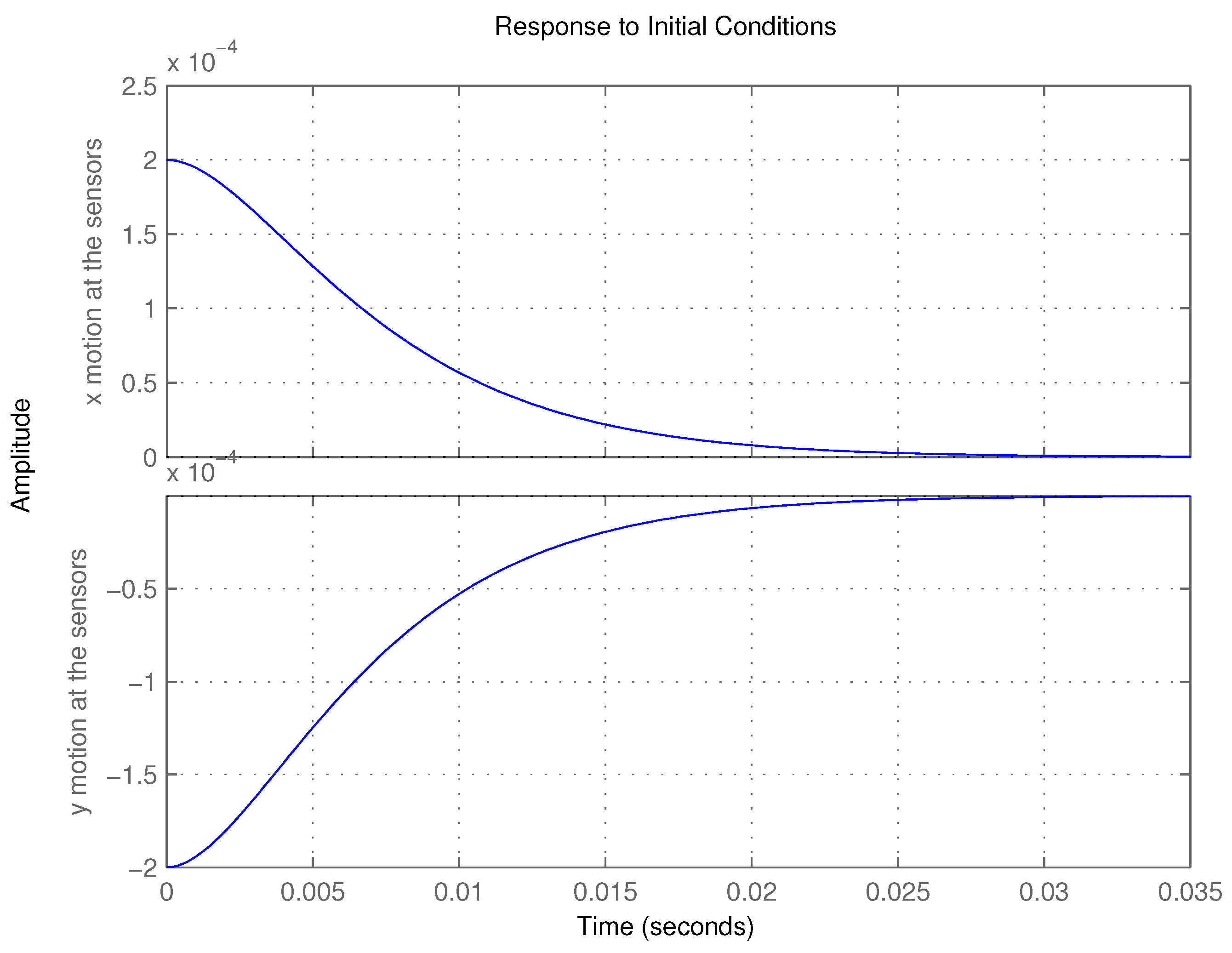
Both cases present a highly damped behavior (very small imaginary part in the eigenvalues). Case B is noticeable faster. The response of Cases A and B to
(
mm),
and zero initial velocities was simulated.
Figure 12 and
Figure 13 show
and
in Cases A and B. Notice that the time scales are different and that Case B is at least two-times faster than Case A. If curves for the required control efforts
u were drawn, the simulations would again show a much faster performance for Type B.
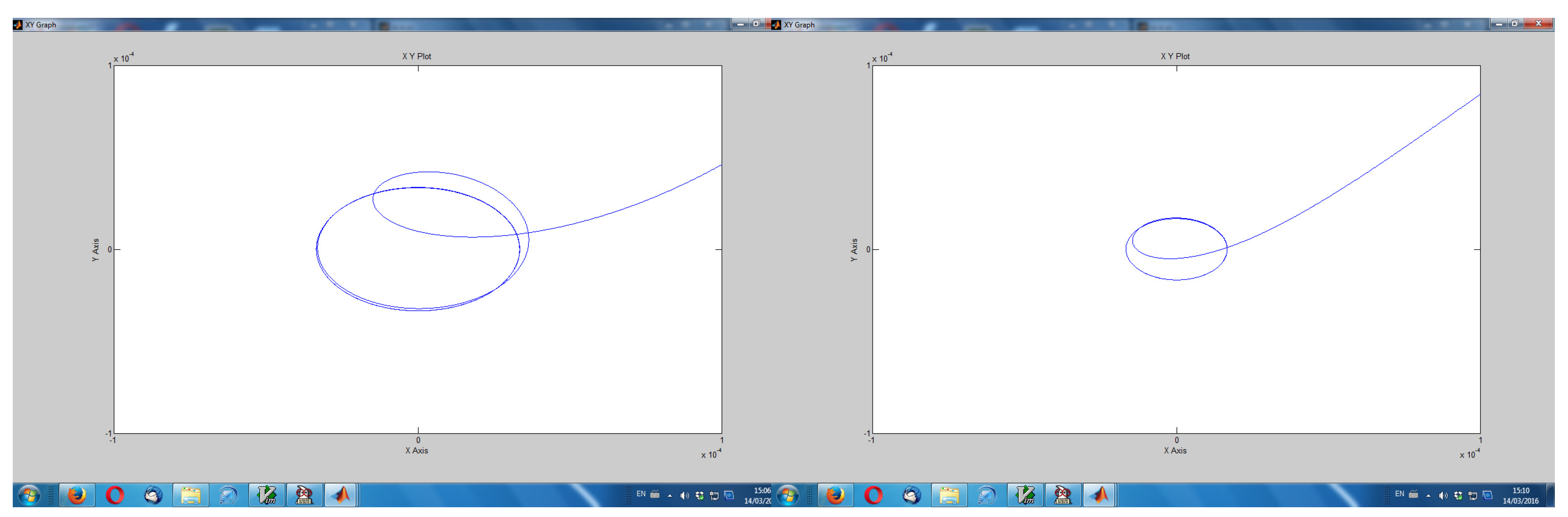
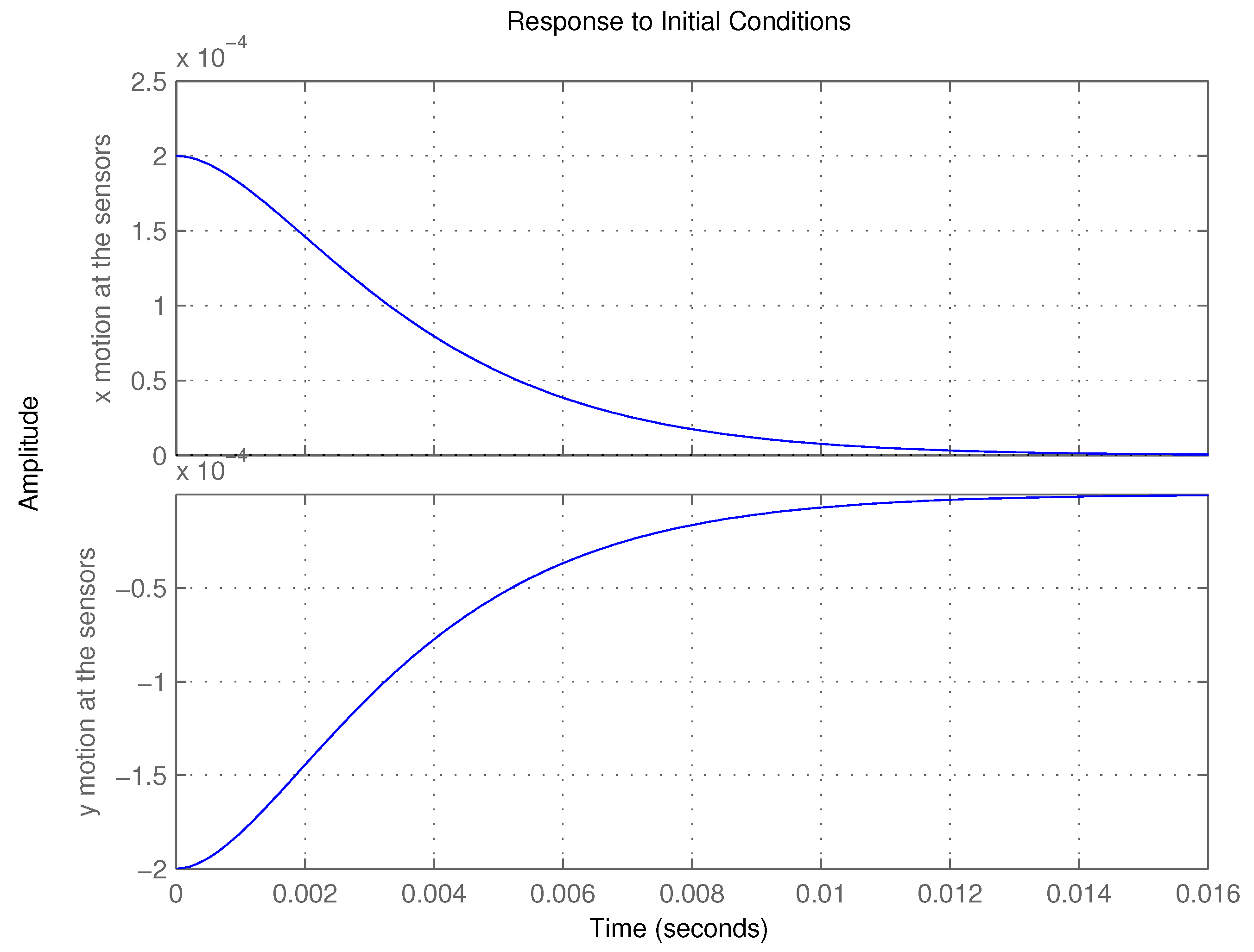
For evaluating the prototypes’ disturbance characteristics, simulations were made for an extra mass of 1 g fixed in the upper disk. The rotor will be unbalanced, and harmonic forces will appear at the
x and
y axes. The resulting disturbance torques will impose orbital movements on the rotor. This means that, for the same initial conditions, the radial displacements will not tend to zero anymore.
Figure 14 shows
plotted against
for Types A (at the left) and B, where the orbits are smaller, characterizing a stiffer suspension behavior, as expected.
These simulations suggest a procedure for laboratory tests on the prototypes: measuring the orbits. In addition to this, a frequency response test was presented in [
13] and is repeated here. Assuming now a constant
rad/s (954 rpm), the state space parameters
and
D are calculated, generating matrices
, etc. A state feedback control law
capable of stabilizing both models can be achieved with:
The resulting closed-loop is described by the eigenvalues of
and
. Simulations, with
F driving models
and
(calculated for a fixed
rad/s) show that both cases are very quickly stabilized, in less than a second. With an extra mass of 1 g fixed in the upper disk, the resulting harmonic forces will impose orbital movements on the rotor, and the overall efficiency of the AMB control can be judged by these orbits, as noted above. A more complex simulation, with the model parameters now depending on
(
and
in (
44) and (
45)), can be performed. For the same stabilizing
F above, and for
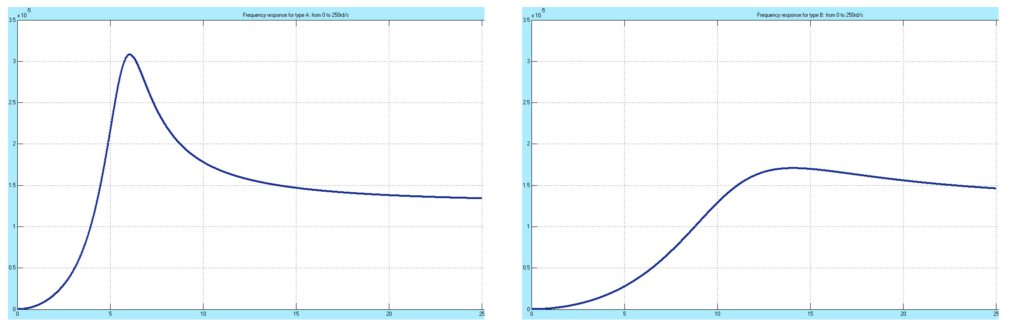
slowly varying from the rest condition to 250 rad/s, the orbit radius for Cases A and B was plotted as function of
; the results are shown in
Figure 15.
The sharp resonance in Model A is almost completely eliminated and shifted to a higher frequency, in Case B. Other control laws can be found that stabilize both models with a better dynamic behavior that avoids resonances in their frequency response. In all of these simulations, Model B offers a clearly superior disturbance rejection characteristic. The bench tests to be made with the real prototypes can follow very closely the procedures used in these simulations.
As a final remark, it must be said that the control laws presented in this section are “special purpose” ones: their main goal is to stabilize the prototypes in a way that the differences between Types A and B are explicitly shown and enhanced. The extremely important problem of choosing control laws for the normal operation of AMBs, either of Type A or B, does not fit in this paper; it belongs to a more control-oriented publication, where lengthy discussions could be made. This future paper could address, for instance, the interesting problem of, with the help of control, making a Type A bearing behave like a Type B.
6. Comments and Conclusions
A detailed mathematical model for Type B is the main contribution of this paper. Its validity, as well as many possible comparisons with Type A, must wait for practical tests. The prototypes are already finished and operational, but no solid measurements have been made up to now. The simulations shown previously confirm the basic assumptions of Type B superiority, but, more than that, they suggest the laboratory procedures to be used in the actual testing of the prototypes.
Some pertinent questions, not treated in this paper, but that will be certainly the object of future research, must be considered. Is the Type B configuration, with its interconnected fluxes, decoupled actions and higher magnetic gains as easy to control with traditional methods as Type A? Are there control laws capable of imposing a Type B behavior on a Type A bearing? Can higher values for and bring undesired effects, like bearing forces that are more sensitive to external disturbances? Will the linearity be affected, with a narrower operating range?
Some other important facts can be considered in future works. It seems obvious that a Type B structure, with only four “poles”, is more compact and, therefore, easier to design and build; its heat dissipation and magnetic loss characteristics are also expected to be superior. If these conjectures are confirmed on the future laboratory tests, a solid advantage for Type B would appear.


