Abstract
A pile foundation in a permafrost region is in a negative-temperature environment, so concrete is affected by the negative temperature of the surrounding soil. It not only affects the formation of concrete strength but also leads to engineering quality accidents in serious cases. With the support of the two permafrost bridge projects of the national highway from Beijing to Mohe in the Greater Khingan Mountains region, a systematic remote dynamic monitoring method for ground temperature in ice-rich tundra is proposed. Based on the actual measurement of temperature at different strata depths and the comprehensive consideration of surface temperature, terrestrial heat flux and other parameters, the ground temperature profile evolution in relation to depth in Greater Khingan was established. The theoretical ground temperature profile curve is similar to the measured profile. The results show that the variation trends of ground temperatures in relation to the strata depth at different monitoring sites is similar, and all show seasonal variation: From June to November, the ground temperature at different depths tends to be constant. From December to May, the ground temperature at any depth within the range of 0 to 5.5 m follows the curve of the cosine function. Below 5.5 m, the earth temperature no longer varies with depth. The research results can be used as reference for pile foundation construction in a negative-temperature environment in ice-rich tundra.
1. Introduction
The Greater and Lesser Khingan Mountains in northeast China belong to degraded perennial island tundra with an area of about 214,600 km2. Permafrost is degrading steadily with the warming of the climate [1]. Meanwhile, the construction of houses and roads required by human beings for living and traveling has artificially intensified the destruction of the permafrost environment with the development of the economy [2,3]. From the perspective of environmental resource protection, it is of great significance to study the variation of ground temperature in relation to the strata depth in perennial island tundra, so as to predict the degradation of the permafrost environment and take timely protection measures [4,5]. Considering the problem of permafrost degradation, bored pile foundations are widely used in highway construction. After pouring concrete, the cast-in-place pile thaws the soil around the pile due to the heat transfer between the concrete and the surrounding soil [6]. At the same time, concrete is affected by the negative temperature of surrounding soil, which affects the formation of concrete strength [7,8] and the quality of concealed works, so there are hidden safety risks in the works. Therefore, the variation of the ground temperature in relation to the strata depth in the permafrost region can be applied to the negative-temperature environment of pile foundation to ensure the engineering quality by selecting an appropriate construction period [9], designing anti-freeze concrete [10,11] and using an insulating layer [10,12,13,14,15].
Domestically and overseas, some progress has been made in the study of the variation of ground temperature in the permafrost region. Hugo et al. [16], Havard et al. [17] and Alice et al. [18] established numerical models of ground temperature on the surface of permafrost. They take into account site factors such as air temperature, snow depth, solar radiation, thermal conductivity, freezing index, etc. in combination with meteorological monitoring data and long-term terrestrial temperature records. According to Andersland [19], in homogeneous soils with a constant state, the surface temperature presents a relatively simple cyclic relationship over a period of one day or one year. This rule that the ground temperature and time follow the trigonometric periodic function has been verified by other scholars, and it has been concluded that the same rule is observed below a certain depth in the seasonal tundra. For example, Liu et al. [20] and Zhang [21] carried out numerical calculation of the ground temperature of permafrost with a nonlinear fitting method based on measured data. Qiu et al. [22] used a one-dimensional steady-state heat conduction equation to calculate the deep temperature of Junggar Basin, which provided an idea for studying the variation of ground temperature in the permafrost region. Zhang et al. [23] studied the variation of ground temperature with time and depth in the non-seasonal tundra area at high latitude and conducted simulation calculation by using the unsteady phase transition temperature field numerical model. Wu et al. analyzed the variation of permafrost temperature at depths of 6–8 m over the Qinghai–Tibet Plateau using monitoring data [24].
Most studies involving ground temperature estimation models have succeeded, to some extent, in calculating the ground temperature. Their algorithms are complicated, and they have many fitting parameters. The method of estimating ground temperature by function is simple and feasible. However, the current research only focuses on the variation of ground temperature with time or depth. This applies to soils with relatively uniform soil quality and low water content, such as those located on a plateau or with sandy soil. The calculation error is very large for ice-rich tundra areas with high water content, especially for middle and high latitude areas with less sunshine. Therefore, it is necessary to establish a simple calculation model applicable to ice-rich tundra, based on a comprehensive consideration of the ground temperature variation in relation to time and the stratum depth. This approach is more convenient and effective in obtaining the variation of surface and shallow ground temperatures. Based on the continuous monitoring of the ground temperature in the ice-rich tundra of the Greater Hinggan region for one year, this paper reveals the variation of the ground temperature with time and depth, and establishes a ground temperature prediction model for this area, in order to provide a reference for pile foundation construction.
2. Experimental Study of Surface and Shallow Ground Temperature
2.1. Measurement Point Arrangement Scheme and Measurement Method
The test site was Mohe county, Heilongjiang province, which is located at the southeast edge of the permafrost region of Eurasia, the northernmost part of China, and the border of China and Russia (Figure 1; 121°07’–124°20’ E, 52°10’–53°33’ N, average altitude 550 m) [25]. There are abundant wetland resources due to the developed water system; the total area is up to 3935 hectares. There is a continuous permafrost with a thickness of 50–100 m [26]. The annual average temperature is about −5.5 °C. The lowest temperature ever recorded is −52.3 °C and the highest is 38.9 °C. The depth of seasonal thawing of test site no. 1 is 0.2–0.3 m, and that of test site no. 2 is about 0.15 m. Under the comprehensive influence of sufficient supply water, poor drainage conditions and a large quantity of plant root humus in soil, the thawing temperature is −0.1 to −0.8 °C according to the measured data of laboratory tests on soil samples in different soil layers. The reduction in particle size helps to lower the thawing temperature. The average annual precipitation is 460.8 mm. The average annual ice period is seven months, which is the time between the beginning and the end of water such as caused by rivers and lakes freezing [27]. In the past 50 years, the temperature in Mohe has risen by 0.357 °C every 10 years. The warming trend is obvious [28].
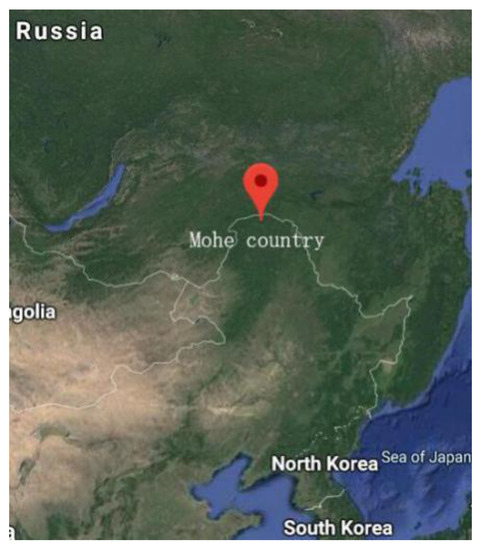
Figure 1.
Geo-localization of the test sites: Mohe county, located on the border between China and Russia.
The two test sites selected in this project were located in the Zhangling–Xilinji section of the national highway from Beijing to Mohe; test site 1 was located between pile 10 and pile 11 of the permafrost bridge under construction (no. K424 + 380), and test site 2 was located between pile 15 and pile 16 of the permafrost bridge under construction (no. K425 + 290). The two test sites were 18.52 km apart. The ground temperature of permafrost in different sites was observed with two temperature measuring tubes. According to the local geological exploration data, the lengths of the two temperature measuring tubes were both designed to be 11.5 m. In order to place temperature sensors in each layer of soil as far as possible, 13 temperature sensors were arranged at different intervals according to the geological survey drawings of the design institute. The distance between adjacent sensors was 0.55–1.45 m. The observation period was from October 2017 to October 2018. In order to monitor the periodic variation of ground temperature in a year, the 20th day of each month was selected for measurement. Since the solar radiation at noon is the most intense, the analysis of ground temperature is more significant, so the temperature collection time was set at 12:00 in this study. Soil layer and temperature measuring point layout are shown in Figure 2.
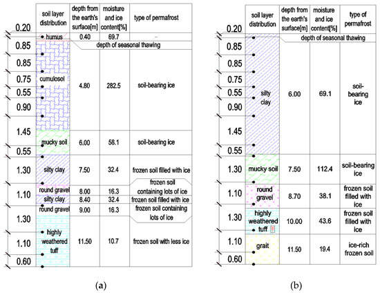
Figure 2.
Distribution of soil layers and temperature measuring point arrangement at different test sites: (a) test site no. 1; (b) test site no. 2.
The temperature monitoring system consists of the lower computer and the upper computer, and the system structure is shown in Figure 3. The lower computer includes temperature sensor, temperature acquisition module, power-control module, wireless transceiver module and seal box. The function of the lower computer is that the temperature acquisition module collects the ground temperature data according to the preset time and transmits the data to the upper computer by means of the point-to-point wireless transmission system of general packet radio service (GPRS) modules. The upper computer includes a computer and a data receiving platform, whose function is to receive data and process the data to generate text files. The most important advantage of the intelligent monitoring system is that the temperature can be dynamically monitored by setting the data acquisition time. The temperature monitoring system adopts an independent solar power supply system to ensure the continuity and stability of the temperature acquisition module under the continuous low temperature environment in winter.
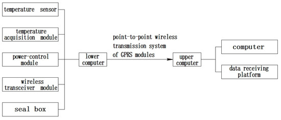
Figure 3.
Schematic diagram of temperature monitoring system.
The temperature sensor adopted a resistance-type temperature-sensing element JMT-36C (Figure 4) and waterproof technology of three-layer sealing protection. The outer shell was made of stainless steel for protection and sealing. The collected temperature range was −40 °C to 150 °C. The accuracy was ±0.2 °C. According to the sensor layout scheme, each temperature measuring wire was tied individually on the outside of the PVC pipe with insulating and waterproof tape, which was then inserted into the pre-dug temperature measuring hole, as shown in Figure 5a,b. Each temperature measuring wire had a thermistor temperature measuring probe. The hole was sealed with fine sand. As the core of this intelligent temperature monitoring system, the temperature acquisition module integrated the main control chip, clock, large-capacity data storage, wireless transmission module, power supply interface, data interface and rechargeable battery, as shown in Figure 5c. The temperature acquisition module could work completely independently. It could automatically complete the measurement of ground temperature and store it in memory according to the preset start time and interval time of measurement, so as to ensure the data were continuous and not lost. When the external battery capacity was insufficient, the rechargeable battery in the temperature acquisition module can continue to be measured regularly. The power-control module included a solar panel and external battery, as shown in Figure 5d. The wireless transmission module was equipped with a mobile phone card and transmitted the data to the upper computer via GPRS. Since the solar radiation is the strongest at noon, the temperature collection time was set at 12:00 every day in this study.
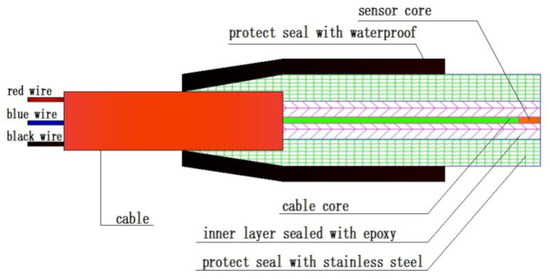
Figure 4.
Internal structure diagram of temperature sensor.
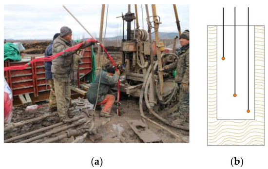
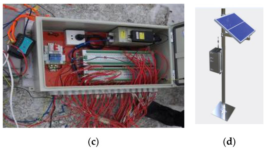
Figure 5.
Temperature monitoring system on site: (a) insertion of the PVC tube with the temperature sensor in the pre-dug hole; (b) schematic diagram of the embedding of temperature measuring wire in hole; (c) temperature acquisition module; (d) solar power system.
2.2. Analysis of Ground Temperature Variation
The curves of temperature changes with depth at the two test sites are shown in Figure 6. By comparing the two figures, it can be seen that the temperature variation of the two test sites was similar, but the temperature variation of each month was quite different and can be divided into three trends. First, the ground temperature decreased significantly followed by a slight rise with the change of depth from December 2017 to March 2018. Moreover, from December to February of the following year, the range of temperature drop increased significantly by month, and the depth of inflection point of the geothermal curve also increased. Taking test site 1 as an example, in December 2017, and January and February 2018, the ground temperature decreased from 11.4 °C, 15.1 °C, and 16.8 °C to −2 °C, 1.8 °C, and 1.9 °C, then fell to 2.7 °C, 2.6 °C, and 2.5 °C, respectively, increasing by 9.4 °C, 13.3 °C and 14.9 °C and only falling by 0.7 °C, 0.8 °C and 0.6 °C. The inflection point of the geothermal curve extended from a depth of 2 to 5.5 m accordingly. Second, in contrast to the last stage, the ground temperature increased first and then decreased with the change of depth from April to October 2018. The range of change in April was relatively small, while the trend of the other months was almost the same. At the depths of 6 and 10 m, the ground temperature fluctuated slightly in a small range of nearby depths. The ground temperature increased slightly at the depth of 5.5 m, while the ground temperature changed from heating to cooling at the depth of 10 m. Third, the ground temperature declined steadily and slowly in October and November 2017. The ground temperature range was 0.4 to −3 °C, showing a trend of slow decline from the surface to a depth of 12 m in October 2017. Since November 2017, the overall trend of ground temperature was linear, but slight temperature fluctuations began to appear after the rise near the surface; in the case of test pile 1, the temperature fell to 0.6 °C at the depth of 1.05 m from 0.9 °C at the depth of 0.2 m, then gradually fell to 2.9 °C at the depth of 12 m. In addition, two months of the year were in the transition stage of temperature change, namely, November 2017 and April 2018. November 2017 was the critical month when the ground temperature started to rise first and then fall, while November 2018 was the critical month when the ground temperature started to fall first and then rise. The measured ground temperature may be different from the natural ground temperature, since the drilling operation in October to November 2017 was at the stage when the permafrost disturbance is the most severe.
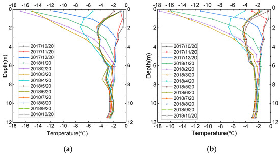
Figure 6.
Monthly ground temperature–depth curve at different test sites: (a) test site 1; (b) test site 2.
2.3. Analysis of Ground Temperature Field in Typical Months
The study region was located in the ice-rich tundra, so the annual variation of the ground temperature is obviously different from that in other regions, and does not completely follow the simple harmonic vibration curve. In other areas, the profile curves of ground temperature and air temperature show a simple harmonic trend, with only the phase and amplitude being different. In winter, the ground temperature of the shallow surface of the region showed a tendency of first decreasing and then rising, and the ground temperature varied greatly at different depths. In summer, the ground temperature of all soil layers did not change dramatically. The monthly temperature change curves of the two test sites with time are shown in Figure 7. As shown in the figures, there were some differences in the monthly temperature variation at different depths, which can be divided into two trends. Large temperature changes were mainly concentrated between November 2017 and June 2018, among which May was the most complex, while the temperature range from June to November 2017 was very small, and the ground temperature change was almost stable. The average annual temperature change curve of the air in this area over the past year is shown in Figure 8. The comparison between Figure 7 and Figure 8 shows that the minimum value of the air temperature was −29.00 °C, which appeared in December. The ground temperature varied with depth, and the minimum value of all soil layers appeared in February, two months later than the air temperature. Air temperatures peaked at 18.65 °C in July. The ground temperature did not display a certain peak like the air temperature but, from May to June, the ground temperature amplitude gradually approached zero. The air temperature changed from negative (−11.57 °C) to positive (1.38 °C) in April, while the ground temperature rose to a constant value in June, and the value of each soil layer was below zero. From the perspective of depth change, it was bounded by 5.5 m. When the depth was less than 5.5 m, the variation range of the ground temperature was obvious from November 2017 to June 2018. Moreover, from the surface down, the range of temperature change gradually decreased with the increase of depth. Moreover, when the depth was greater than 5.5 m, the variation range of the ground temperature in each month of the year was relatively small.
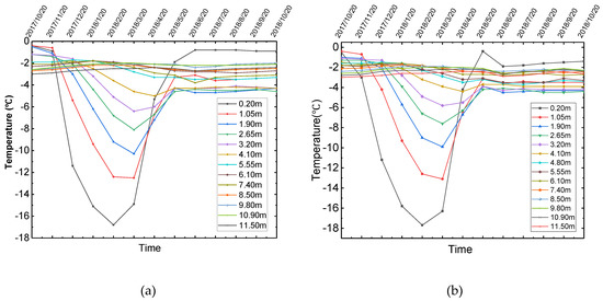
Figure 7.
Ground temperature–time curve at different test sites: (a) test site 1; (b) test site 2.
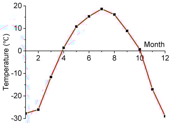
Figure 8.
Air temperature–time curve at Mohe.
As can be seen from Figure 8, even at a depth of 20 cm the soil temperature in summer did not reach 0 °C, and the depth of seasonal thawing was about 0.15–0.3 m. There are two reasons for this: First, the geological feature of the study area is the ice-rich tundra in the mountains. It is located in a basin of high latitude mountains, and is a vast wetland with significant moisture and ice content, in which even the soil is always saturated all year round. Both study areas have supplemental water near them; site 1 is fed by a lake and site 2 is fed by a patch of perennial snow in a nearby forest. The slow thawing process continued throughout the summer, generating a large amount of phase transition latent heat. The water released by thawing remains in the sticky soil layer dominated by cumulosol and silty clay, and is almost impossible to drain. A large amount of ice and water coexist for a long time. Second, the area is extremely rich in water resources, so surface vegetation has developed. Moss, ferns and other plants rapidly reproduce in summer. In particular, the thick Carex tato, which grows in the peaty soil in the swamp of the Hinggan Mountains, plays a good role in preventing solar radiation and heat insulation.
3. Prediction Model of Ground Temperature of Permafrost
The assumptions of the model are [19,28]: (1) the heat transfer process can be approximately regarded as the unsteady heat conduction process of a semi-infinite object under the periodic boundary conditions; (2) there is no temporary non-climatic disturbance on the surface, such as geothermal disturbance, groundwater, etc.; (3) the system disturbance can be ignored (for example, the thermal properties of soil remain unchanged).
According to the heat conduction theory, under the condition of the surface temperature changing periodically, the change curve of ground temperature in a permafrost region at any depth and time is [19]:
where: is the average annual temperature of the earth’s surface; is the amplitude of surface temperature; is the depth; is the ground temperature monitoring date, starting from January 1 of the current year (for example, 28 February 2018 is the 59th day of the year, so ); is the time when the initial phase of the surface temperature wave occurs; is the period; is the comprehensive parameter of permafrost; , where is the thermal diffusion coefficient of permafrost.
Solar radiation is the main factor influencing the surface temperature distribution in the shallow layer [20]. The data showed that the temperature change within 1 d had little effect on the surface temperature of the shallow layer. However, the 1-year solar radiation change had a significant impact [21]. Considering that the shallow ground temperature can reach equilibrium within one year, the 1-year cycle is adopted in this study, taking .
According to the analysis of the temperature and time curve, the temperature distribution curve can be approximately regarded as a simple harmonic in the time range . In the time range , the linear trend is parallel to the horizontal axis, and the intersection point between the line and the Y-axis is considered to be the ground temperature constant value C1 corresponding to the month when the permafrost phase transition is severe. The temperature wave equation of 1 year in a permafrost region is as follows:
In the time range , according to the analysis of the geothermal and depth curve of this project, the temperature field distribution curve can be approximately regarded as a simple harmonic wave in the depth range . In the depth range , the linear trend is parallel to the vertical axis, and the intersection point between the line and the X-axis is considered to be the annual average ground temperature depth C2.
where and represent the average annual temperature of the rocks of the corresponding time and depth respectively, which are constant; is the depth of zero annual amplitudes; is the gradient of terrestrial heat flow, which is mainly used for linear correction of terrestrial heat flow to ground temperature.
Under the background of global warming, the ground temperature in the permafrost region is also increasing by year.
Assuming that the ground temperature increases at a constant speed and the growth rate is , then the ground temperature curve model on day of the Nth year is as follows:
where is the year of ground temperature curve fitting.
4. Verification of Ground Temperature Prediction Model
It can be seen from Figure 7 that during the period from June to November 2018, the ground temperature of the permafrost in this project stabilized at −1.5 °C to −4.5 °C. It can be discarded in the calculation because the ground temperature at a depth of 0.2 m from the surface is greatly disturbed by surface factors. The numerical mean value of the ground temperature at each point at the depth of 1.05–11.5 m is −3.0 °C. In other months, there were similar simple harmonic forms of temperature, and the data were substituted into Equation (2) to obtain Equation (5). As can be seen from Figure 7, the variation of ground temperature in February is larger than that in other months. If the ground temperature of other months is calculated by the formula of February, the calculated value is safer. Therefore, the ground temperature monitored on 20 February 2018 is selected in this paper to fit the ground temperature curve of this region. According to the daily data of “ground temperature at 0 cm” published by the national meteorological center, and values were calculated and substituted into Equation (5) to obtain Equation (6).
The permafrost is not uniform in relation to the depth, and the physical indexes of permafrost are different in every soil layer. The K values at different depths of the project are shown in Figure 9. The thermal diffusion coefficient is needed to calculate the comprehensive parameters of permafrost. The value of thermal diffusion coefficient was obtained by sampling soil from each soil layer on site (Figure 2) and then measured by heat transfer analyzer (Figure 10).
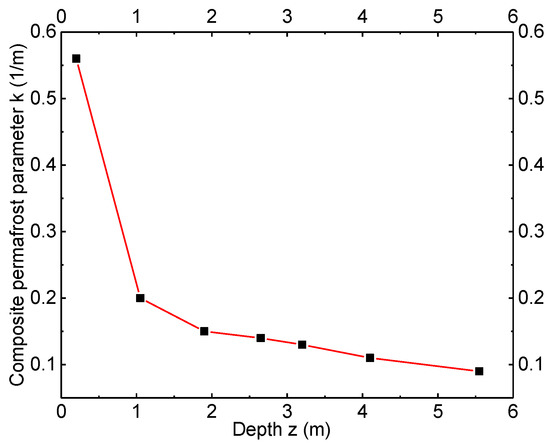
Figure 9.
Curve of comprehensive parameters of permafrost changing with depth.
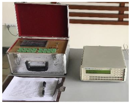
Figure 10.
Model 2104 heat transfer analyzer.
The average growth rate of ground temperature in the region where the project is located is 0.03–0.04 °C per year [25,29]. As can be seen from Figure 6, the depth of zero annual average amplitudes is 5.5 m, and the full depth prediction model of the ground temperature curve is finally obtained, as shown in Equation (7). The measured ground temperature data and the calculated value of the fitting curve are drawn as a ground temperature and depth curve, as shown in Figure 11. It can be seen from Figure 10 that the predicted ground temperature curve is in good agreement with the measured ground temperature curve, and the fitting accuracy of the formula is high. It shows that the proposed method to characterize the equation and evolution model of the temperature fluctuation curve of permafrost is feasible, and the calculation results are reliable. It can provide theoretical support for the design of permafrost bridge pile foundations and subgrade in the Hinggan mountains region.
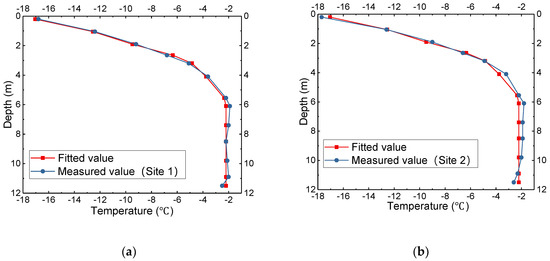
Figure 11.
The measured curve of ground temperature and fitting results: (a) test site 1; (b) test site 2.
5. Discussion
For the surface and shallow ground temperature distribution of permafrost, a simplified heat conduction formula expressed by a simple harmonic equation is used to match the measured temperature, which is a commonly used distribution theory [19,20,21,22]. However, none of these equations pay attention to the seasonal characteristics of ground temperature under the latent heat of phase transition in ice-rich tundra. The ice-rich tundra has a high water content. It was found that the water content of cumulosol at test pile 1 was as high as 282.5%. One key finding is that the distribution of the temperature profile in the ice-rich tundra in middle and high latitudes is quite different from the traditional equation due to the alternations of ice cover and melting in different seasons.
From June to October every year, surface and shallow ground temperature is at the level of zero annual amplitude, which is different from the variation of surface temperature (Figure 11a). It does not conform to the simple harmonic curve. During this period, due to heavy precipitation and lack of snow and ice cover, solid ice and hygroscopic water, thin film water, capillary water, gravity water and other liquid water exist between soil particles at the same time, and the solid–liquid phase conversion occurs when water penetrates into the underground soil and the soil water content increases. Because of the latent heat of phase transition, there is heat transfer but no temperature change. From November to May of the next year, precipitation is small, as shown in Figure 11b. Meanwhile, a blanket of snow and ice blocks solar radiation. As the temperature decreases, the content of solid ice in permafrost continues to increase, and the latent heat of phase transition no longer plays a dominant role. Therefore, the surface and shallow surface temperatures are affected by atmospheric temperature according to a simple harmonic law.
Permafrost, located 5.5 m below the surface of the earth, is not affected by complex factors such as solar radiation and atmospheric temperature change all the year round. Therefore, free water such as confined water and binding water between molecules exists in the form of solid–liquid coexistence for a long time. Therefore, the ground temperature is constant except for the occasional small change of ground temperature at the interface of different viscous soils.
It should be noted that the daily value of earth temperature may lead to the deviation of fitting parameters, as the study adopted the 12:00 instantaneous value instead of the daily average temperature. In addition, since the measurement period is only one year, it is necessary to gradually improve the fitting equation by excluding accumulated data.
6. Conclusions
This study draws the following conclusions:
- (1)
- In the Hinggan mountains region of Mohe county, a remote monitoring system of ground temperature in ice-rich tundra was developed. The system used solar panels and low temperature resistant batteries to supply power and adapt to the characteristics of low temperature in the Hinggan mountains region. The function of real-time remote monitoring was realized using temperature transmission module and GPRS point-to-point wireless transmission. The waterproof temperature sensor was adopted to meet the characteristics of high moisture and ice content in the ice-rich tundra.
- (2)
- The nonlinear fitting method was used to obtain the ground temperature curve fitting model with a 1-year cycle. In the ice-rich tundra of the Hinggan mountains, the ground temperature profile evolution does not completely obey the simple harmonic curve. From June to November, the ground temperature at each depth tends to be constant. In the depth range of 0 to 5.5 m from December to May, the ground temperature at any depth follows the curve of a cosine function. Below 5.5 m, the ground temperature no longer varies with depth but tends to the normal value. By comparing the prediction model of the ground temperature fluctuation curve of permafrost at any depth with the field monitoring data, the reliability of the model is verified. It is proved that this fitting model is feasible to characterize the variation of permafrost temperature in relation to the depth of the stratum.
- (3)
- The permafrost is not uniform in relation to the depth, and the physical indexes of permafrost are different in different soil layers. When calculating the ground temperature, it is suggested to use the data according to the curve of the relationship between comprehensive parameter and depth of permafrost, so as to effectively reduce the error.
Author Contributions
Conceptualization, T.Y. and Z.L.; Methodology, T.Y. and Z.L.; Software, Z.L. and N.Y.; Validation, Z.L. and N.Y.; Investigation and experiment, L.G. and Z.L.; Resources, T.Y.; Data Curation, Z.L. and N.Y.; Writing and Visualization, Z.L. All authors have read and agreed to the published version of the manuscript.
Funding
This work was funded by Basic Scientific Research Operating Expenses of Central Universities (No. 2572015BB03), Longjian Road and Bridge Co., LTD. Science and Technology Project (No. LJKY004-2017).
Acknowledgments
The author would like to thank the Northeast Forestry University Forest and its supervisor for valuable suggestions to facilitate this project. We would like to thank the editor and the anonymous reviewers for their work. Thanks to China meteorological data information center for providing relevant data.
Conflicts of Interest
The author declares no conflict of interest.
References
- Zhang, X.; Yang, F.; Leng, Y.; Xue, Y. Permafrost Test and Investigation of Frost Damage; Science Press: Beinjing, China, 2013; pp. 4–5. [Google Scholar]
- Zhou, Y.; Guo, D.; Qiu, G.; Cheng, G. China’s Permafrost; Science Press: Beijing, China, 2000; pp. 40–41. [Google Scholar]
- Xie, D. Design and construction of a gas pipeline in frozen soil. Soil Eng. Found. 2016, 30, 355. [Google Scholar]
- Tan, Y.; Wang, X.; Wang, Y. Progress of wetland researches in cold regions china. J. Glaciol. Geocryo. 2011, 33, 197–201. [Google Scholar]
- Lu, X.; Liu, Y.; Bian, H.; Sun, Z.; Wang, C.; Qiu, X. The Application of Extruded Polystyrene Boards in Frost Heaving Prevention of ConcreteLining Channel. J. Shandong Agri. Univ. 2019, 50, 460–467. [Google Scholar]
- Liu, N.; Li, N.; He, M.; Xu, S. Analyzing the factors controlling the bearing capacity of cast-in-place piles based on a thermo-hydro-mechanical coupling model. J. Glaciol. Geocryol. 2014, 36, 1471–1477. [Google Scholar]
- Jiang, S.; Dong, S.; Zhu, W.; Li, H.; Yin, S. Study on freezing critical strength of concrete with negative temperature based on compressive strength. China Concr. Cem. Prod. 2019, 10, 24–26. [Google Scholar]
- Dai, J.; Wang, Q.; Xie, Z.; Zhang, P.; Tian, Z.; Zhang, B. Influence factors of strength growth of equal strength concrete under −3 °C curing. J. Lanzhou Jiaotong Univ. 2018, 37, 14–19. [Google Scholar]
- Wang, X.; Jiang, D.; Liu, D.; He, F. Experimental study of bearing characteristics of large-diameter cast-in-place bored pile under non-refreezing condition in low-temperature permafrost ground. Chin. J. Rock Mech. Eng. 2013, 32, 1807–1812. [Google Scholar]
- Zhang, Y.; Xie, Y.; Li, Y.; Zhao, F. Rationality of heat preservation mode in cold region tunnels and model test verification. J. Railw. Sci. Eng. 2016, 13, 1569–1576. [Google Scholar]
- Xie, H.; He, C.; Li, Y. Study on insulating layer thickness by phase-change temperature field of highway tunnel in cold region. Chin. J. Rock Mech. Eng. 2007, 26, 4395–4401. [Google Scholar]
- Xia, C.; Fan, D.; Han, C. Precewise calculation method for insulation layer thickness in cold region tunnels. Chin. J. Highw. Transp. 2013, 26, 131–138. [Google Scholar]
- Geng, L.; Jin, Y.; Wu, C.; Ling, X.; Du, X.; Wang, X. Analysis of thermal insulation and frost prevention of Dongxing swelling rock tunnel at Jilin-Tumen-Hunchun highspeed railway. J. Nat. Disasters 2019, 28, 17–25. [Google Scholar]
- Hu, T.; Wang, T.; Liu, J.; Chang, J. Design and experiment on a solar heat-supplying tube against frost damage of embankment in cold regions. Chin. Civil Eng. J. 2019, 52, 44–52. [Google Scholar]
- Yan, H. Experimental study on thermal insulation technique to prevent subgrade frost-heaving for high speed railway in seasonal frozen soil region. Railway Eng. 2019, 59, 1–4. [Google Scholar]
- Beltrami, H.; Kellman, L. An examination of short and long-term air-ground temperature coupling. Global Planet. Chang. 2003, 38, 291–303. [Google Scholar] [CrossRef]
- Juliussen, H.; Humlum, O. Towards a TTOP ground temperature model for mountainous terrain in central-eastern Norway. Permafr. Periglac. Process. 2007, 18, 161–184. [Google Scholar] [CrossRef]
- Ferreira, A.; Vieira, G.; Ramos, M.; Nieuwendam, A. Ground temperature and permafrost distribution in Hurd Peninsula (Livingston Island, Maritime Antarctic): An assessment using freezing indexes and TTOP modelling. Catena 2017, 149, 560–571. [Google Scholar] [CrossRef]
- Orlando, B.A.; Branko, L. Frozen Ground Engineering, 2nd ed.; China Architecture and Building Press: Beijing, China, 2001; p. 196. [Google Scholar]
- Liu, D.; Wang, S.; Jin, L. Permafrost ground temperature fitting model of Gonghe-Yushu highway. Chin. J. Highw. Transp. 2015, 28, 100–105. [Google Scholar]
- Zhang, D. Study on the evolution law of permafrost ground temperature. Geotech. Invest. Surv. 2019, 1, 41–45. [Google Scholar]
- Qiu, N.; Wang, X.; Yang, H.; Xiang, Y. The characteristics of temperature distribution in the Junggar Basin. Chin. J. Geol. 2001, 36, 350–358. [Google Scholar]
- Zhang, Y.; Du, Y.; Sun, B. Temperature distribution in roadbed of high-speed railway in seasonally frozen regions. Chin. J. Rock Mech. Eng. 2014, 33, 1286–1296. [Google Scholar]
- Wu, Q.; Liu, Y. Ground temperature monitoring and its recent change in Qinghai-Tibet Plateau. Cold Regions Sci. Tech. 2004, 38, 85–92. [Google Scholar]
- Lu, Y.; Yu, W.; Guo, M.; Liu, W. Spatiotemporal variation characteristics of land cover and land surface temperature in Mohe county, Heilongjiang province. J. Glaciol. Geocryol. 2017, 39, 1137–1149. [Google Scholar]
- Jin, H.; Yu, Q.; Lü, L.; Yu, S. Degradation of permafrost in the Xing’anling Mountains, Northeastern China. Permafr. Periglac. Proc. 2007, 18, 245–258. [Google Scholar] [CrossRef]
- Chen, L.; Yu, W.; Yi, X.; Wu, Y.; Ma, Y. Application of ground penetration radar to permafrost survey in Mohe County, Heilongjiang Province. J. Glaciol. Eocryol. 2015, 37, 723–730. [Google Scholar]
- Liu, Y.; Gao, Z.; Liang, J. Heat Transfer Theory; China Electric Power Press: Beijing, China, 2015; pp. 22, 165–166. [Google Scholar]
- Yu, W.; Guo, M.; Chen, L. Influence of urbanization on permafrost: a case study from Mohe County, Northernmost China. Cryosphere Discuss. 2014, 8, 4327–4348. [Google Scholar] [CrossRef]
© 2020 by the authors. Licensee MDPI, Basel, Switzerland. This article is an open access article distributed under the terms and conditions of the Creative Commons Attribution (CC BY) license (http://creativecommons.org/licenses/by/4.0/).