

The Possibility of Estimating the Permafrost’s Porosity In Situ in the Hydrocarbon Industry and Environment

1
Department of Geophysics, Faculty of Exact Sciences, Tel Aviv University, Ramat Aviv, Tel Aviv 6997801, Israel
2
Azerbaijan State Oil and Industry University, 20 Azadlig Ave., Baku AZ1010, Azerbaijan
Geosciences 2024, 14(3), 72; https://doi.org/10.3390/geosciences14030072
Submission received: 22 January 2024
/
Revised: 6 March 2024
/
Accepted: 8 March 2024
/
Published: 9 March 2024
(This article belongs to the Topic Natural Hazards and Environmental Challenges in the Anthropocene Age)
Abstract
:Global warming firstly influences the permafrost regions where numerous and rich world hydrocarbon deposits are located. Permafrost thawing has caused severe problems in exploring known hydrocarbon deposits and searching for new targets. This process is also dangerous for any industrial and living regions in cold regions. Knowledge of permafrost’s ice and unfrozen water content is critical for predicting permafrost behavior during the water–ice transition. This is especially relevant when ice and permafrost are melting in many regions under the influence of global warming. It is well known that only part of the formation’s pore water turns into ice at 0 °C. After further lowering the temperature, the water phase transition continues, but at gradually decreasing rates. Thus, the porous space is filled with ice and unfrozen water. Laboratory data show that frozen formations’ mechanical, thermal, and rheological properties strongly depend on the moisture content. Hence, porosity and temperature are essential parameters of permafrost. In this paper, it is shown that by combining research in three fields, (1) geophysical exploration, (2) numerical modeling, and (3) temperature logging, it is possible to estimate the porosity of permafrost in situ. Five examples of numerical modeling (where all input parameters are specified) are given to demonstrate the procedure. This investigation is the first attempt to quantitatively analyze permafrost’s porosity in situ.
1. Introduction
Thawing permafrost because of global warming creates severe problems in the cold regions of industrial development [1], including areas of hydrocarbon searching and exploration [2]. For successive hydrocarbon exploration in cold regions and prospecting for new deposits, it is helpful to know some permafrost parameters (firstly, porosity) [3]. Thawing permafrost also creates specific difficulties for industrial and residential areas e.g., Refs. [4,5,6]. Therefore, constant monitoring of permafrost porosity under global warming conditions is necessary [7,8,9]. The relationship between the porosity and the permeability of hydrate-bearing sediments (that can cause massive release of methane gas into the atmosphere) has been shown by Majorowicz et al. [10] and Liu et al. [11,12].
It is well known that only a part of the formation’s pore water turns into ice at 0 °C. With the additional lowering of the temperature, the phase transition of the water continues, however, at gradually decreasing rates. The quantity of unfrozen water is practically independent of the total moisture content for soil with concrete physical–chemical parameters [13]. Frozen soil is the matter in which stresses and strains arise under the influence of an external load. These forces are not constant but vary with time. They give rise to the relaxation of stresses and creeps (i.e., increased strains over time). These complex physical–chemical processes are called rheological ones. The vigorous development of rheological processes in frozen soils is caused by the peculiarities of their internal relationships in which ice plays a significant role. Numerous laboratory experiments show that frozen formations’ mechanical, thermal, and rheological properties strongly depend on the moisture content. Hence, porosity and temperature are essential parameters of permafrost. It is known that the electric resistivities of frozen sediments are affected by the freezing–thawing transition to a greater extent than the seismic velocities. In the same interval of temperatures, seismic velocities may increase by 2 to 10 times in transition to frozen conditions, whereas the electrical resistivity may increase by 3 × 10²–103 times [14,15,16]. The position of the thawing–freezing transition interface can be determined by applying the surface electric resistivity method and sonic logs in wells. For instance, the transition from higher resistivity and velocity values to lower ones can be considered the thawing radius’s position. Thus, the position of the radius of thawing (because of well drilling or production) can be estimated using different geophysical exploration methods. A method of estimating the refreezing time surrounding thawed (during drilling) wellbore formations was suggested by Kutasov and Eppelbaum [17,18]. Only three temperature logs taken after the freeze-back were completed and are needed to apply this method. The conducted numerical modeling indicates that the dimensionless time of refreezing can be expressed as a function of two dimensionless parameters: radius of thawing and latent heat density [3,19]. From the last parameter, the porosity of formations can be estimated.
The only objective of this study is to offer a possible way to estimate permafrost’s porosity in situ. This study is the first effort to determine this parameter in natural conditions. This in situ parameter estimation is particularly important when the permafrost parameters constantly change under the influence of global warming. Five cases of numerical modeling are presented to demonstrate the possibility of the applicability of this new method.
2. Time of Freeze-Back
Since deep-well drilling in permafrost areas usually uses warm mud, a certain unknown degree of the formation of thawing around the wells exists. The warm mud disturbs the borehole’s temperature field, and as a result, the permafrost thaws. To calculate the static formation temperature and permafrost thickness, before conducting temperature logs, engineers must wait for some period after the entire completion of drilling. The duration of the refreezing of the layer thawed during drilling dramatically depends on the natural temperature of geological formation(s). Therefore, the rocks at the bottom of the permafrost zone freeze very slowly. A lengthy restoration period (up to ten years or more) is required to calculate the permafrost’s temperature and thickness with the necessary accuracy.
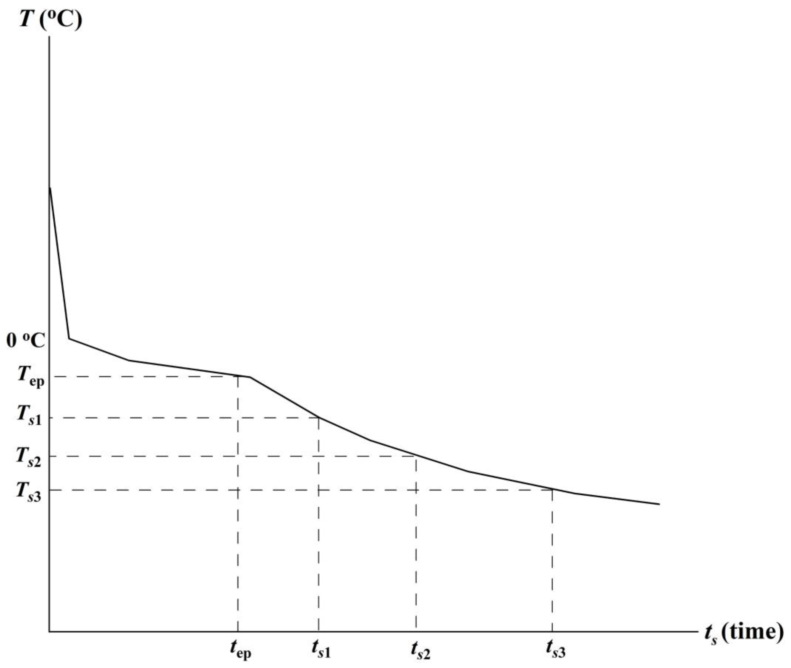
As mentioned above, only a part of the formation’s pore water changes to ice at 0 °C. The phase transition temperature interval exists in numerous laboratory and field experiments. With the subsequent lowering of the temperature, the water phase transition continues (Figure 1). The temperature interval of the phase transition mainly depends on the mineralogical composition of the geological formations. Let us assume that the water–ice phase transition is completed at the time tep, and at least three temperature logs are taken after refreezing thawed formations (Figure 1).
Kutasov and Eppelbaum [17,18,20] have shown that the cooling process at t > tep (Figure 1) is like that of temperature recovery in borehole sections below the permafrost base (i.e., unfrozen formations). Let us assume that thermal recovery’s starting point is t = tep. Thus, the thermal disturbance time is td + tep, where td is the time of drilling mud circulation at a given depth. It will be explained below that the subsequent borehole cooling can be approximated by a constant linear heat source (per unit of length) after refreezing.
Hence, a modified Horner equation (in some publications, this method is called KEM (for instance, [21,22]) can be used to predict frozen formations’ temperature to estimate the formation temperature [17,18]. Then,
Combining Equations (2)–(4), Equation (5) is obtained to estimate the time of refreezing (tep).
For solving Equation (5), Newton’s method was used [23]. In this method, a solution to an equation is obtained by defining a s of numbers that become successively nearer and nearer to the expected solution [17,18].
The parameter B is found from the following equation:
Furthermore, the temperature of formations can be obtained from Equations (2)–(4).
3. The Empirical Formula
It was assumed that the heat flow influence from the thawed zone to the thawed zone–frozen zone interface could be neglected. The results of hydrodynamical modeling have established that this is an acceptable assumption [24,25]. In this case, the Stefan equation—energy conservation condition at the phase change interface (r = h)—can be applied:
Assuming the semi-steady temperature distribution in the frozen zone (a conventional assumption),
where rif is the radius of thermal influence during the freeze-back period. The ratio Df = rif/h was obtained from a numerical solution. A computer program [24] was used to find a numerical solution for a system of differential heat conductivity equations for frozen and thawed zones and the Stefan equation. It was found that
where If is the dimensionless latent heat density, L is the latent heat per unit of mass, cf is the specific heat of the formation, φ is the porosity, ρw is the water density, ρf is the formation density, ro is the borehole radius, h is the radius of thawing, and λf and af are the thermal conductivity and diffusivity of the frozen formations, respectively.
1.5 < If ≤ 400, 1.25 < H < 23.4, H = h/ro,
From Equations (7)–(9) and the condition H(tep) = 1, the following was obtained [19]:
where tepD is the dimensionless time of refreezing.
4. Numerical Modeling: Five Cases
Taylor [26] introduced a cylindrically symmetric source of thermal disturbance in a semi-infinite medium to analyze thermal borehole measurements. A numerical model was developed to simulate the rising transient thermal regime in the mentioned model. The assumed medium is a permafrost sandstone formation. The model allows for a phase change (ice–water, water–ice). In this model, only heat transfer by radial conduction is considered. The following parameters are introduced: the radius of cylindrical source ro = 0.17 m, the radial variable r, the thermal conductivity of frozen formation λf = 4.40 Wm−1 K−1, the thermal conductivity of unfrozen formation λun = 3.84 Wm−1 K−1, specific heat cf = 950, cun = 1138 Jkg−1 K−1, the density of sandstone ρf = 2483 kg m−3, the density of water/ice ρw = 1000 kg m−3, the porosity φ = 0.09, and the latent heat L = 334,960 J kg−1 for the water–ice boundary. The latent heat density of the medium is χ = Lρwφ = 334,960 · 1000 · 0.09 = 30 · 106 Jm−3. The duration of source disturbance is td. The temperature of 0 °C is assumed as a phase change. The calculated data in Table 1, Table 2, Table 3 and Table 4 are given for initial temperatures (Tf) of −0.01°, −5°, and −10 °C and for source temperatures of (Tw): 10 °C and 30 °C. In the construction of Table 1, Table 2, Table 3 and Table 4, dimensionless distance and dimensionless time were used:
Thus, td is the time of thermal disturbance and ts is the “shut-in” time. The radial temperature distributions during the thermal disturbance (Td) and “shut-in” (Ts) periods are presented as follows:
5. Results of Calculations
At this stage, to use Equations (1)–(6), the following parameters will be replaced
by the dimensionless values
The results of calculations after Equations (1)–(6) (in the dimensionless units) are presented in Table 3 and Table 4 (columns 4–6).
As can be seen from Table 3 for case 1, the calculated dimensionless refreezing time varies in the restricted limits (18.5–21.3). At the same time, the results of numerical modeling provide corresponding values of 20–30 (Table 1, values in bold). For cases 2–5, the calculated refreezing times (Table 3 and Table 4, column 4) agree with the results of mathematical modeling (Table 1 and Table 2, values in bold).
The dimensionless thawing radius was defined as the position of the 0 °C isotherm and was found from Td = f (R, tdD) as 0 °C = f (R = H, tdD). Here, linear interpolation was used.
From Equation (11), it follows that the dimensionless latent heat density (If) can be determined as a function of dimensionless refreezing time and thawing radius. As with the solution of implicit Equation (6), Newton’s method was again used to estimate the value of If from Equation (11). The calculation results are presented in Table 3 and Table 4 (column 7).
Finally, the porosity is found in Equation (10):
It also should be noted that for cases 1, 2, 4, and 5, the calculated values of formation temperature (Table 3 and Table 4, column 6) are in excellent agreement with the assumed values (Tf = −5 °C and −10 °C) from numerical modeling. The difference Tf − Tfcal for case 3 can be explained by the low accuracy in determining the radius of thawing. As mentioned earlier, the linear interpolation method was used to estimate the thawing radius. Figure 2 also shows that the basic Equation (1) (in dimensionless units) can be used to estimate the transient shut-in temperature.
6. Discussion and Conclusions
The estimated porosity (φ) values are presented in Table 3 and Table 4 (column 8). For case 1, the φ values vary in narrow limits of 0.086–0.095. The ranges for cases 2–5 are 0.088–0.109, 0.081–0.011, 0.096–0.102, and 0.084–0.091, respectively. Thus, the average porosity values in all five cases are very close to the assumed numerical modeling value of φ = 0.09. The results of calculations shown in Table 3 and Table 4 (columns 4–8) testify that the basic formulas 1, 5, and 11 approximate the results of the numerical modeling with the necessary accuracy.
It should be noted that all input parameters (i.e., dimensionless heating and “shut-in” time, latent heat density, and thermal properties of the formation) were specified in numerical modeling. Only the dimensionless thawing radius was defined as the position of the 0 °C isotherm and was found from tables Td = f (R, tdD) as 0 °C = f (R = H, tdD). From the implicit Equation (11), it follows that the dimensionless latent heat density is a function of two parameters: dimensionless thawing radius (H) and dimensionless refreezing time (tepD). Thus, to estimate the porosity of permafrost in field conditions (in situ), it is essential to determine the values H and tepD by temperature logging and other geophysical methods. Industrial companies should not encounter difficulties in the use of geophysical methods in the exploration and development of oil and gas fields. For this reason, this work can be considered a preliminary study in this field.
The proposed methodology was calculated for the case of porosity = 0.09. The following testing of the suggested approach for high porosities will illustrate its applicability for estimating the potential of natural hydrate-bearing sediments [27,28].
As mentioned earlier, the position of the interface of the thawing–freezing transition (radius of thawing) can be verified with geophysical methods—sonic logs and electric resistivity. Kutasov and Eppelbaum [17,18] presented three examples of estimation of the refreezing time using temperature logging results. Furthermore, to validate the approach presented in this paper, the calculated porosity values should be compared with those obtained from cuttings and samples.
Funding
This research received no external funding.
Data Availability Statement
The data is contained within the article.
Acknowledgments
The author would like to thank the anonymous reviewers who thoroughly reviewed the manuscript. Their critical comments and valuable suggestions were constructive in preparing this paper.
Conflicts of Interest
The authors declare no conflict of interest.
References
- Hjort, J.; Streletskiy, D.; Doré, G.; Wu, Q.; Bjella, K.; Luoto, M. Impacts of permafrost degradation on infrastructure. Nat. Rev. Earth Environ. 2022, 3, 24–38. [Google Scholar] [CrossRef]
- Langer, M.; von Deimling, T.S.; Westermann, S.; Rolph1, R.; Rutte, R.; Antonova, S.; Rachold, V.; Schultz, M.; Oehme, A.; Grosse, G. Thawing permafrost poses environmental threat to thousands of sites with legacy industrial contamination. Nat. Commun. 2023, 14, 1721. [Google Scholar] [CrossRef] [PubMed]
- Eppelbaum, L.V.; Kutasov, I.M. Well drilling in permafrost regions—Dynamics of the thawed zone. Polar Res. 2019, 38, 1–9. [Google Scholar] [CrossRef]
- Creamean, J.M.; Hill, T.C.J.; DeMott, P.J.; Uetake, J.; Kreidenweis, S.; Douglas, T.A. Thawing permafrost: An overlooked source of seeds for Arctic cloud formation. Environ. Res. Lett. 2020, 15, 084022. [Google Scholar] [CrossRef]
- van Huissteden, J. Thawing Permafrost. In Permafrost Carbon in a Warming Arctic; Springer Nature Switzerland AG: Cham, Switzerland, 2020; 520p. [Google Scholar]
- Murton, J.B. Permafrost and climate change. In Climate Change, 3rd ed.; Letcher, T.M., Ed.; Elsevier: Amsterdam, The Netherlands, 2021; pp. 281–326. [Google Scholar] [CrossRef]
- Koven, C.D.; Riley, W.J.; Stern, A. Analysis of permafrost thermal dynamics and response to climate change in the CMIP5 earth system models. J. Clim. 2013, 26, 1877–1900. [Google Scholar] [CrossRef]
- Boike, J.; Chadburn, S.; Martin, J.; Zwieback, S.; Althuizen, I.H.J.; Anselm, N.; Cai, L.; Coulombe, S.; Lee, H.; Liljedahl, A.K.; et al. Standardized monitoring of permafrost thaw: A user-friendly, multiparameter protocol. Arct. Sci. 2021, 8, 153–182. [Google Scholar] [CrossRef]
- Tomaškovičová, S.; Ingeman-Nielsen, T. Coupled thermo-geophysical inversion for permafrost monitoring. Cryosphere 2024, 18, 321–340. [Google Scholar] [CrossRef]
- Majorowicz, J.; Osadetz, K.; Safanda, J. Onset and stability of gas hydrates under permafrost in an environment of surface climatic change—Past and future. In Proceedings of the 6th International Conference on Gas Hydrates (ICGH 2008), Vancouver, BC, Canada, 6–10 July 2008; pp. 1–14. [Google Scholar]
- Liu, L.; Dai, S.; Ning, F.; Caie, J.; Liu, C.; Wu, N. Fractal characteristics of unsaturated sands—Implications to relative permeability in hydrate-bearing sediments. J. Nat. Gas Sci. Eng. 2019, 66, 11–17. [Google Scholar] [CrossRef]
- Liu, L.; Zhang, Z.; Li, C.; Ning, F.; Liu, C.; Wu, N.; Cai, J. Hydrate growth in quartzitic sands and implication of pore fractal characteristics to hydraulic, mechanical, and electrical properties of hydrate-bearing sediments. J. Nat. Gas Sci. Eng. 2020, 75, 103109. [Google Scholar] [CrossRef]
- Tsytovich, N.A. The Mechanics of Frozen Ground; Scripta Book Co.: Washington, DC, USA, 1975; 426p. [Google Scholar]
- Hnatiuk, J.; Randall, A.G. Determination of permafrost thickness in wells in Northern Canada. Canad. J. Earth Sci. 1977, 14, 375–383. [Google Scholar] [CrossRef]
- Dobinski, W. Permafrost. Earth-Sci. Rev. 2011, 108, 158–169. [Google Scholar] [CrossRef]
- Eppelbaum, L.V. VLF-method of geophysical prospecting: A non-conventional system of processing and interpretation (implementation in the Caucasian ore deposits). ANAS Trans. Earth Sci. 2021, 16–38. [Google Scholar] [CrossRef]
- Kutasov, I.M.; Eppelbaum, L.V. Time of refreezing of surrounding the wellbore thawed formations. Int. J. Therm. Sci. 2017, 122, 133–140. [Google Scholar] [CrossRef]
- Kutasov, I.M.; Eppelbaum, L.V. WITHDRAWN: Corrigendum to “Time of refreezing of surrounding the wellbore thawed formations” [Int. J. Thermal Sci. 122 (December 2017) 133–140]. Intern. J. Therm. Sci. 2018, 124, 548. [Google Scholar] [CrossRef]
- Kutasov, I.M. Radius of thawing around an injection well and time of complete freezback. J. Geophys. Eng. 2006, 3, 154–159. [Google Scholar] [CrossRef]
- Kutasov, I.M.; Eppelbaum, L.V. Prediction of formation temperatures in permafrost regions from temperature logs in deep wells—field cases. Permafr. Periglac. Process. 2003, 14, 247–258. [Google Scholar] [CrossRef]
- Bassam, A.; Santoyo, E.; Andaverde, J.; Hernández, J.A.; Espinoza-Ojeda, O.M. Estimation of static formation temperatures in geothermal wells by using an artificial neural network approach. Comput. Geosci. 2010, 36, 1191–1199. [Google Scholar] [CrossRef]
- Liu, C.; Li, K.; Chen, Y.; Jia, L.; Ma, D. Static Formation Temperature Prediction Based on Bottom Hole Temperature. Energies 2016, 9, 646. [Google Scholar] [CrossRef]
- Grossman, S.I. Calculus; Elsevier: Amsterdam, The Netherlands, 2014; 1148p. [Google Scholar]
- Kutasov, I.M. Applied Geothermics for Petroleum Engineers; Elsevier: Amsterdam, The Netherlands, 1999; 346p. [Google Scholar]
- Eppelbaum, L.V.; Kutasov, I.M.; Pilchin, A.N. Applied Geothermics; Springer: Berlin/Heidelberg, Germany, 2014; 751p. [Google Scholar]
- Taylor, A.E. Temperatures and Heat Flow in a System of Cylindrical Symmetry Including a Phase Boundary; Geothermal Series 7; Energy Mines Resources: Ottawa, ON, Canada, 1978; 95p.
- Li, Y.; Liu, L.; Jin, Y.; Wu, N. Characterization and development of natural gas hydrate in marine clayey-silt reservoirs: A review and discussion. Adv. Geo-Energy Res. 2021, 5, 75–86. [Google Scholar] [CrossRef]
- Wan, Y.; Yuan, Y.; Zhou, C.; Liu, L. Multiphysics coupling in exploration and utilization of geo-energy: State-of-the-art and future perspectives. Adv. Geo-Energy Res. 2023, 10, 7–13. [Google Scholar] [CrossRef]
Figure 1.
Shut-in temperatures at a given depth—schematic curve.

Figure 2.
Transient shut-in temperature. Case 1, B = 3.39 °C, Tfcal = −10 °C, tdD = 100, tepD = 18.5. The solid line is constructed using Equation (1); points present the numerical modeling results.
Figure 2.
Transient shut-in temperature. Case 1, B = 3.39 °C, Tfcal = −10 °C, tdD = 100, tepD = 18.5. The solid line is constructed using Equation (1); points present the numerical modeling results.


Table 1.
Input data for 2 cases of numerical modeling ([26], pp. 56, 57). Tw is the temperature of the cylindrical source, Ts is the shut-in temperature, and Tf is the temperature of formation.
Table 1.
Input data for 2 cases of numerical modeling ([26], pp. 56, 57). Tw is the temperature of the cylindrical source, Ts is the shut-in temperature, and Tf is the temperature of formation.
| Case 1 | Case 2 | ||
| Tw = 10 °C, | Tw = 10 °C, | ||
| Tf = −10 °C, | Tf = −10 °C, | ||
| tdD = 100 | tdD = 300 | ||
| tsD | Ts, °C | tsD | Ts, °C |
| 20 | 0.00 | 30 | 0.00 |
| 30 | 0.00 | 60 | −1.19 |
| 40 | −3.32 | 90 | −4.24 |
| 50 | −4.52 | 120 | −5.29 |
| 70 | −5.80 | 150 | −5.96 |
| 100 | −6.81 | 210 | −6.80 |
| 200 | −8.18 | 300 | −7.53 |
| 300 | −8.72 | 400 | −8.02 |
| 400 | −9.01 | 500 | −8.34 |
| 500 | −9.19 | 600 | −8.57 |
| 600 | −9.31 | 700 | −8.74 |
| 700 | −9.41 | 1700 | −9.47 |
| 800 | −9.48 | ||
| 900 | −9.53 | ||
Table 2.
Input data for three cases of numerical modeling ([26], pp. 73, 50, 65).
Table 2.
Input data for three cases of numerical modeling ([26], pp. 73, 50, 65).
| tsD | Ts, °C | tsD | Ts, °C | tsD | Ts, °C |
| Case 3 | Case 4 | Case 5 | |||
| Tw = 30 °C, | Tw = 10 °C, | Tw = 30 °C, | |||
| Tf = −10 °C, | Tf = −5 °C, | Tf = −5 °C, | |||
| tdD = 1000 | tdD = 30 | tdD = 30 | |||
| 400 | 0.0 | 30 | 0.0 | 60 | 0.0 |
| 500 | 0.0 | 40 | 0.0 | 70 | 0.0 |
| 700 | −3.52 | 50 | −1.22 | 170 | −2.58 |
| 800 | −4.45 | 60 | −2.32 | 270 | −3.66 |
| 900 | −5.09 | 70 | −2.61 | 370 | −4.05 |
| 1000 | −5.58 | 170 | −4.15 | 470 | −4.27 |
| 2000 | −7.93 | 270 | −4.46 | 570 | −4.40 |
| 3000 | −8.91 | 370 | −4.61 | 670 | −4.49 |
| 4000 | −9.43 | 470 | −4.69 | 770 | −4.56 |
| 5000 | −9.70 | 570 | −4.74 | 870 | −4.61 |
| 970 | −4.65 | ||||
Table 3.
Results of calculations for cases 1 and 2. Tfcal is the calculated formation temperature. Input data are presented in Table 1.
Table 3.
Results of calculations for cases 1 and 2. Tfcal is the calculated formation temperature. Input data are presented in Table 1.
| 1 | 2 | 3 | 4 | 5 | 6 | 7 | 8 |
| ts1D | ts2D | ts3D | tepD | B, °C | Tfcal, °C | If | Φ |
| Case 1. H = 3.87; Tf = −10°C | |||||||
| 50 | 70 | 900 | 18.5 | 3.49 | −9.97 | 1.205 | 0.086 |
| 50 | 70 | 800 | 18.5 | 3.50 | −9.97 | 1.205 | 0.086 |
| 50 | 70 | 700 | 18.5 | 3.49 | −9.97 | 1.205 | 0.086 |
| 50 | 70 | 600 | 18.7 | 3.46 | −9.95 | 1.217 | 0.087 |
| 50 | 70 | 500 | 18.7 | 3.46 | −9.95 | 1.217 | 0.087 |
| 50 | 70 | 400 | 18.8 | 3.45 | −9.95 | 1.223 | 0.087 |
| 50 | 70 | 300 | 19.1 | 3.43 | −9.93 | 1.241 | 0.089 |
| 50 | 70 | 200 | 19.6 | 3.37 | −9.89 | 1.272 | 0.091 |
| 40 | 70 | 200 | 21.3 | 3.25 | −9.86 | 1.375 | 0.098 |
| 40 | 70 | 300 | 20.9 | 3.31 | −9.91 | 1.351 | 0.096 |
| 40 | 70 | 400 | 20.7 | 3.34 | −9.93 | 1.339 | 0.096 |
| 40 | 70 | 500 | 20.6 | 3.35 | −9.94 | 1.333 | 0.095 |
| 40 | 70 | 600 | 20.5 | 3.36 | −9.94 | 1.327 | 0.095 |
| Case 2. H = 4.80; Tf = −10 °C | |||||||
| 90 | 120 | 210 | 37.5 | 2.78 | −9.81 | 1.525 | 0.109 |
| 90 | 120 | 300 | 36.7 | 2.82 | −9.85 | 1.494 | 0.107 |
| 90 | 120 | 400 | 35.9 | 2.86 | −9.89 | 1.464 | 0.105 |
| 90 | 120 | 500 | 35.6 | 2.87 | −9.90 | 1.452 | 0.104 |
| 90 | 120 | 600 | 35.4 | 2.89 | −9.92 | 1.445 | 0.103 |
| 90 | 120 | 700 | 35.3 | 2.89 | −9.92 | 1.441 | 0.103 |
| 90 | 120 | 1700 | 33.3 | 3.00 | −10.02 | 1.364 | 0.097 |
| 120 | 210 | 300 | 32.0 | 2.96 | −9.92 | 1.314 | 0.094 |
| 120 | 210 | 400 | 30.4 | 3.01 | −9.94 | 1.252 | 0.089 |
| 120 | 210 | 500 | 30.3 | 3.02 | −9.95 | 1.248 | 0.089 |
| 120 | 210 | 600 | 29.9 | 3.03 | −9.95 | 1.233 | 0.088 |
| 120 | 210 | 700 | 30.0 | 3.03 | −9.95 | 1.237 | 0.088 |
Table 4.
Results of calculations for cases 3–5. Tfcal is the calculated formation temperature. Input data are presented in Table 2.
Table 4.
Results of calculations for cases 3–5. Tfcal is the calculated formation temperature. Input data are presented in Table 2.
| 1 | 2 | 3 | 4 | 5 | 6 | 7 | 8 | |||
| ts1D | ts2D | ts3D | tepD | B, °C | Tfcal, °C | If | φ | |||
| Case 3. H = 14.99; Tf = −10 °C | ||||||||||
| 700 | 900 | 2000 | 382.9 | 4.16 | −10.50 | 1.533 | 0.110 | |||
| 700 | 900 | 3000 | 348.9 | 4.62 | −10.81 | 1.405 | 0.100 | |||
| 700 | 900 | 4000 | 336.5 | 4.98 | −10.92 | 1.359 | 0.097 | |||
| 700 | 900 | 5000 | 338.6 | 4.77 | −10.90 | 1.366 | 0.098 | |||
| 800 | 900 | 2000 | 334.1 | 4.56 | −10.61 | 1.349 | 0.096 | |||
| 800 | 900 | 3000 | 291.3 | 5.10 | −10.90 | 1.186 | 0.085 | |||
| 800 | 900 | 4000 | 277.4 | 5.29 | −10.99 | 1.133 | 0.081 | |||
| 800 | 900 | 5000 | 282.9 | 5.22 | −10.96 | 1.154 | 0.082 | |||
| 700 | 1000 | 5000 | 311.8 | 5.02 | −10.94 | 1.265 | 0.090 | |||
| Case 4. H = 3.94; Tf = −5 °C | ||||||||||
| 60 170 | 570 | 45.8 | 1.11 | −5.01 | 2.704 | 0.096 | ||||
| 60 270 | 570 | 46.5 | 1.09 | −5.01 | 2.742 | 0.098 | ||||
| 60 370 | 570 | 48.8 | 1.00 | −4.99 | 2.868 | 0.102 | ||||
| Case 5. H = 6.42; Tf = −5 °C | ||||||||||
| 270 470 | 970 | 118.4 | 1.491 | −4.99 | 2.544 | 0.091 | ||||
| 270 570 | 970 | 113.7 | 1.550 | −5.00 | 2.451 | 0.088 | ||||
| 270 670 | 970 | 109.0 | 1.611 | −5.00 | 2.356 | 0.084 | ||||
Disclaimer/Publisher’s Note: The statements, opinions and data contained in all publications are solely those of the individual author(s) and contributor(s) and not of MDPI and/or the editor(s). MDPI and/or the editor(s) disclaim responsibility for any injury to people or property resulting from any ideas, methods, instructions or products referred to in the content. |
© 2024 by the author. Licensee MDPI, Basel, Switzerland. This article is an open access article distributed under the terms and conditions of the Creative Commons Attribution (CC BY) license (https://creativecommons.org/licenses/by/4.0/).
Share and Cite
MDPI and ACS Style
Eppelbaum, L.V. The Possibility of Estimating the Permafrost’s Porosity In Situ in the Hydrocarbon Industry and Environment. Geosciences 2024, 14, 72. https://doi.org/10.3390/geosciences14030072
AMA Style
Eppelbaum LV. The Possibility of Estimating the Permafrost’s Porosity In Situ in the Hydrocarbon Industry and Environment. Geosciences. 2024; 14(3):72. https://doi.org/10.3390/geosciences14030072
Chicago/Turabian StyleEppelbaum, Lev V. 2024. "The Possibility of Estimating the Permafrost’s Porosity In Situ in the Hydrocarbon Industry and Environment" Geosciences 14, no. 3: 72. https://doi.org/10.3390/geosciences14030072
Note that from the first issue of 2016, this journal uses article numbers instead of page numbers. See further details here.