

Thermal Anomalies Observed during the Crete Earthquake on 27 September 2021
by
 and
and
Soujan Ghosh
1,*, 
Sudipta Sasmal
2,
Sovan K. Maity
2,3,
Stelios M. Potirakis
4,5,6 and
Masashi Hayakawa
7,8 1
National Atmospheric Research Laboratory, Department of Space, Government of India, Gadanki 517112, India
2
Institute of Astronomy Space and Earth Science, Kolkata 700054, India
3
Uttar Amtala Gita Rani Vidyabhawan (H.S.), Contai 721427, India
4
Department of Electrical and Electronics Engineering, University of West Attica, Ancient Olive Grove Campus, Egaleo, GR-12244 Athens, Greece
5
Institute for Astronomy, Astrophysics, Space Applications and Remote Sensing, National Observatory of Athens, Metaxa and Vasileos Pavlou, Penteli, GR-15236 Athens, Greece
6
Department of Electrical Engineering, Computer Engineering and Informatics, School of Engineering, Frederick University, CY-1036 Nicosia, Cyprus
7
Hayakawa Institute of Seismo-Electromagnetics Co., Ltd. (Hi-SEM), UEC (University of Electro-Communications), Alliance Center 521, 1-1-1 Kojima-cho, Chofu, Tokyo 182-0026, Japan
8
Advanced Wireless and Communications Research Center (AWCC), UEC, 1-5-1 Chofugaoka, Chofu, Tokyo 182-8585, Japan
*
Author to whom correspondence should be addressed.
Geosciences 2024, 14(3), 73; https://doi.org/10.3390/geosciences14030073
Submission received: 6 November 2023
/
Revised: 19 February 2024
/
Accepted: 4 March 2024
/
Published: 9 March 2024
(This article belongs to the Special Issue Lithosphere-Atmosphere-Ionosphere Coupling during Earthquake Preparation: Recent Advances and Future Perspectives)
Abstract
:This study examines the response of the thermal channel within the Lithosphere–Atmosphere–Ionosphere Coupling (LAIC) mechanism during the notable earthquake in Crete, Greece, on 27 September 2021. We analyze spatio-temporal profiles of Surface Latent Heat Flux (SLHF), Outgoing Longwave Radiation (OLR), and Atmospheric Chemical Potential (ACP) using reanalysis data from the National Oceanic and Atmospheric Administration (NOAA) satellite. Anomalies in these parameters are computed by removing the background profile for a non-seismic condition. Our findings reveal a substantial anomalous increase in these parameters near the earthquake’s epicenter 3 to 7 days before the main shock. The implications of these observations contribute to a deeper understanding of the LAIC mechanism’s thermal channel in seismic events.
1. Introduction
Various complicated and nonlinear processes govern the interaction of the lithosphere, atmosphere, and ionosphere. Studying various channels, like chemical, thermal, acoustics, and electromagnetic channels, it was found that precursory earthquake activities begin around a month before the actual catastrophe within the area known as the “preparation zone”. These channels cover a wide range of parameters that can be treated as potential tools to understand the seismogenic effects from beneath the earth’s surface to the magnetospheric heights [1]. These pre-earthquake activities involve complex, heterogeneous, multidimensional, and multi-parametric physical and chemical processes [1,2,3,4,5]. So, the precursory framework of seismic hazards includes a variety of chemical, thermal, acoustic, mechanical, and electromagnetic events, each with its own set of characteristics. Based on these characteristics and their interconnecting properties, a unified theory called Lithospheric–Atmospheric–Ionospheric Coupling (LAIC) has been proposed to explain the coupling that occurs across different layers of the atmosphere and ionosphere during seismic events through a variety of channels, e.g., [1,6,7]. This idea has been addressed and validated in light of the significant variabilities in several atmospheric and ionospheric parameters. This mechanism establishes the inter-relationships between various geochemical and geophysical processes related to earthquake occurrences. Radon emanation [8] is the most commonly accepted possible primary cause of air ionizations in the near-surface area, where the early geochemical and physical processes begin. Ion clusters are created when the ions generated by this mechanism interact with water molecules. These nanometer-sized cluster ions are then released into the atmosphere, changing the natural profile of air conductivity and, as a result, the ionospheric potential also changes [7,9]. These ongoing changes are therefore reflected in the ionosphere as seismogenic ionospheric disturbances, as shown by [10,11,12,13,14,15,16,17,18,19,20,21]. In the lower atmosphere, the condensation of water molecules owing to a change in the relative humidity of air eventually leads to latent heat release. The latent heat release raises in the lower atmosphere are the total energy budget, which initiates the emission of the Outgoing Longwave Radiation flux (W/m2) as measured on the topside of the atmosphere during and prior to seismic events. These thermal anomalies are observed from both ground-based and satellite observations [14,22,23].
It is well established that during the final stage of the earthquake preparation process, the system tends to move to a self-organizing state from a chaotic state to reach the critical state where one can expect the maximum instability in the strain energy profile that is about to go through an avalanche, and after that it passes the system to another quality [24]. Using nonlinear thermodynamics and synergetics, these processes can be described [25]. Some integral parameters with threshold values mainly describe the system. When the parameter crosses the threshold value, the system approaches the critical state. This threshold is the final stage of the earthquake preparation and rupture processes in the seismogenic process. Furthermore, the integral parameter describes several simultaneous processes that lead the system to the critical state. The chemical potential of water vapor at a high ionization level is one of the probable candidates to be the integral parameter during the seismogenic process, as its values are derived from the anomalies in both the atmospheric temperature and humidity.
Pulinets et al. [26] presented that during the phase transition, the latent heat required by the water molecule is equivalent to its chemical potential. In multicomponent media with external forcing, the relative humidity can be represented as
where , and is the volume averaged correction of chemical potential, arising from external forcing of the environment. The square of the cosine of time represents the diurnal variation in the intensity of the solar radiation, and represents the boiling temperature. is a complex parameter reflecting the formation of cluster ions. A higher value of indicates that the energy of the water molecule binding with ions is also higher, and the cluster ions are more stable. These stable cluster ions have a much longer lifetime and grow larger due to the attachment of water molecules.
Gorny et al. [27] first observed prominent signatures for thermal anomalies in the Central Asian region. They analyzed a satellite image of the earth’s surface within the spectral range of 10.5–11.3 over some linear structures of the Middle Asian seismically active region (Kopet Dagh, Talasso-Ferghana, and other faults) and observed positive anomalies of IR radiation along the point of intersection of the Talasso-Ferghana and Tamdy-Tokrauss faults. After that, several researchers started to study thermal anomalies associated with large earthquakes using various parameters in China, Japan, India, Iran, and Algeria [28,29,30,31,32,33]. Pulinets et al. [34] presented that Atmospheric Chemical Potential (ACP) anomalies are generated in the last stage of the seismic cycle. The temporal variation in the ACP is very similar to the radon activity in the preparation zone. The magnitude of the ACP drops close to the moment of the main shock. This magnitude of the ACP variation is weaker over the ocean. It was also found that there are areas where ACP anomalies are very weak or negative variation is observed. Pulinets et al. [35] presented the importance of ACP anomalies before seismogenic activities and other atmospheric phenomena.
In our study, we chose the Crete earthquake of 2021 to investigate the possible pre- and co-seismic thermal anomalies from the satellite data and present them with the conventional spatio-temporal variation in the anomalies by removing the background variation in the non-seismic condition. Our main aim is to find the anomaly variation of various parameters related to thermal channels before earthquakes to establish the hypothesis of a possible coupling mechanism during pre-seismic conditions. This work emphasizes one of the most important channels of the LAIC mechanism. The earthquake under study was chosen in such a way that evidence of such seismogenic impression is already established by using other parameters of other channels of LAIC [36]. This will also enable us to study and compare a multi-parametric approach of LAIC mechanisms [37,38,39,40,41]. The plan of this paper is as follows: In Section 2, we present our observations and the methods of extracting anomalies; in Section 3, we present the results and discuss our results; and finally, in Section 4, we make concluding remarks.
2. Data and Methodologies
In our study, we chose the Crete earthquake of 2021 to investigate the possible pre- and co-seismic irregularities of thermal parameters. On 27 September 2021, at 06:17 UT, an earthquake of magnitude struck the island of Crete, Greece, at a depth of 6 km. In Figure 1, we present the epicenter of the earthquake, marked with a tiny red circle; the earthquake preparation zone, marked with a black circle; and the earthquake fault line, marked with a red curve. We present the details of the earthquake in Table 1.
2.1. Surface Latent Heat Flux Anomaly
To identify thermal anomalies related to earthquakes, we first removed the diurnal, seasonal variation, and other meteorological variations. We computed the background data using the seismically quiet period for the same grid area. To compute the background data, we used the following equation:
Here, is the background SLHF as a function of latitude (x), longitude (y), and time (t) and is the background flux. For the studied case, the value of N is 3. We computed the background data for the Crete earthquake using the years 2015, 2017, and 2019, which were seismically quiet. We removed the background variation from the seismically active time period to compute the anomaly as
where is the data obtained for the seismically active time period.
2.2. Outgoing Longwave Radiation Data Analysis
Several researchers have used techniques to analyze Outgoing Longwave Radiation (OLR) data; one of the most significant ones is the Eddy Field Calculation Mean method. This method detects the presence of any singularities in OLR data between adjacent points within the epicenter region [14,42,43,44]. The Eddy Field Calculation Mean is defined as the “total sum of the difference value” of the “measured value” of OLR between adjacent points [45]. This method compares the parameters for one particular point over the grid data with their nearest adjacent grid locations (latitudinal and longitudinal directions). The sum of the difference values of all measured values gives the parameter value for that particular point. Finally, an interpolated values gives the spatio-temporal profile of the said parameter. This method of computation can be expressed as follows:
where is the daily Eddy field, is the daily mean, and x and y are the latitude and longitude, respectively. i and j are the integers representing the number of grids.
2.3. Atmospheric Chemical Potential Analysis
To compute the ACP, we followed the method suggested by Boyarchuk et al. [46]. The authors expressed with the air temperature at the earth’s surface and relative humidity. is expressed as
where is in eV.
In this study, we used data obtained from the National Oceanic and Atmospheric Administration (NOAA) reanalysis dataset. NOAA reanalysis data were taken from https://www.esrl.noaa.gov (accessed on 11 March 2023). These datasets data formats and classes were previously discussed in several publications, e.g., [22]. For the Crete earthquake, we used the latitude range 31° N to 39° N and the longitude range of 20° E to 30° E for the spatio-temporal variation. We computed the anomalies in all these parameters and overlaid the world map over the results to recognize the spatio-temporal variation regarding the epicenter of the earthquake. This showed a systematic variation over both space and time of the analyzed parameters to find out their temporal evolution and the most affected area that shows the maximum perturbation around the EQ epicenter.
3. Results
3.1. Surface Latent Heat Flux Observational Results
In Figure 2 and Figure 3, we present the spatio-temporal variation in Surface Latent Heat Flux (SLHF) anomalies in W/m2. This spatio-temporal variation gives direct evidence of the increase in the SLHF. We present the SLHF anomalies from 13 September 2021 to 12 October 2021, from longitudinal and latitudinal spans from 20° E to 30° E and 31° N to 39° N, respectively. The epicenter is indicated with a red dot and marked with the letter “C”. Figure 2 and Figure 3 show that the sudden intensification of the SLHF anomaly was observed near the epicenter on 23 September 2021. The next day, the maximum intensification of the SLHF anomaly was observed over the epicenter. The anomaly also propagated towards the southeast direction on that particular day. From 25 September, no such anomalous behavior of the SLHF was observed near the epicenter. From 30 September to 6 October, a slight increase in the SLHF anomaly is observed within the preparation zone of the earthquake. These increments in the SLHF are due to aftershocks followed by the mainshock and also due to the combined effect of the earthquake of 12 October, which occurred very close to the epicenter of the first earthquake.
3.2. OLR Results
Figure 4 and Figure 5 represent the daily OLR variation around the earthquake epicenter. Figure 4 shows the OLR variation from 13 to 27 September 2021, whereas in Figure 4, we present the same from 28 September to 12 October 2021. From Figure 4, it is clearly found that the OLR variation was low from 13 to 17 September. On 18 September, the OLR increased near the northern part of the earthquake preparation zone. The maximum intensification was observed on 20 September. The OLR variation decreased in the next few days and again started increasing on 23 September near the earthquake’s epicenter. From 24 September, it started decreasing and completely vanished on 25 September. In Figure 5, we see that the OLR again increased during the first week of October due to aftershocks and the combined effect of another mainshock that occurred on 12 October, south-southeast of Crete island [12 October 2021, 09:24:04.8 UT, (34.894° N, 26.472° N), , depth = 10 km], near the epicenter of the earthquake under study. It is also found that on the day of the second earthquake, the maximum intensification of OLR variation was observed within the region close to the epicenter.
3.3. ACP Variation
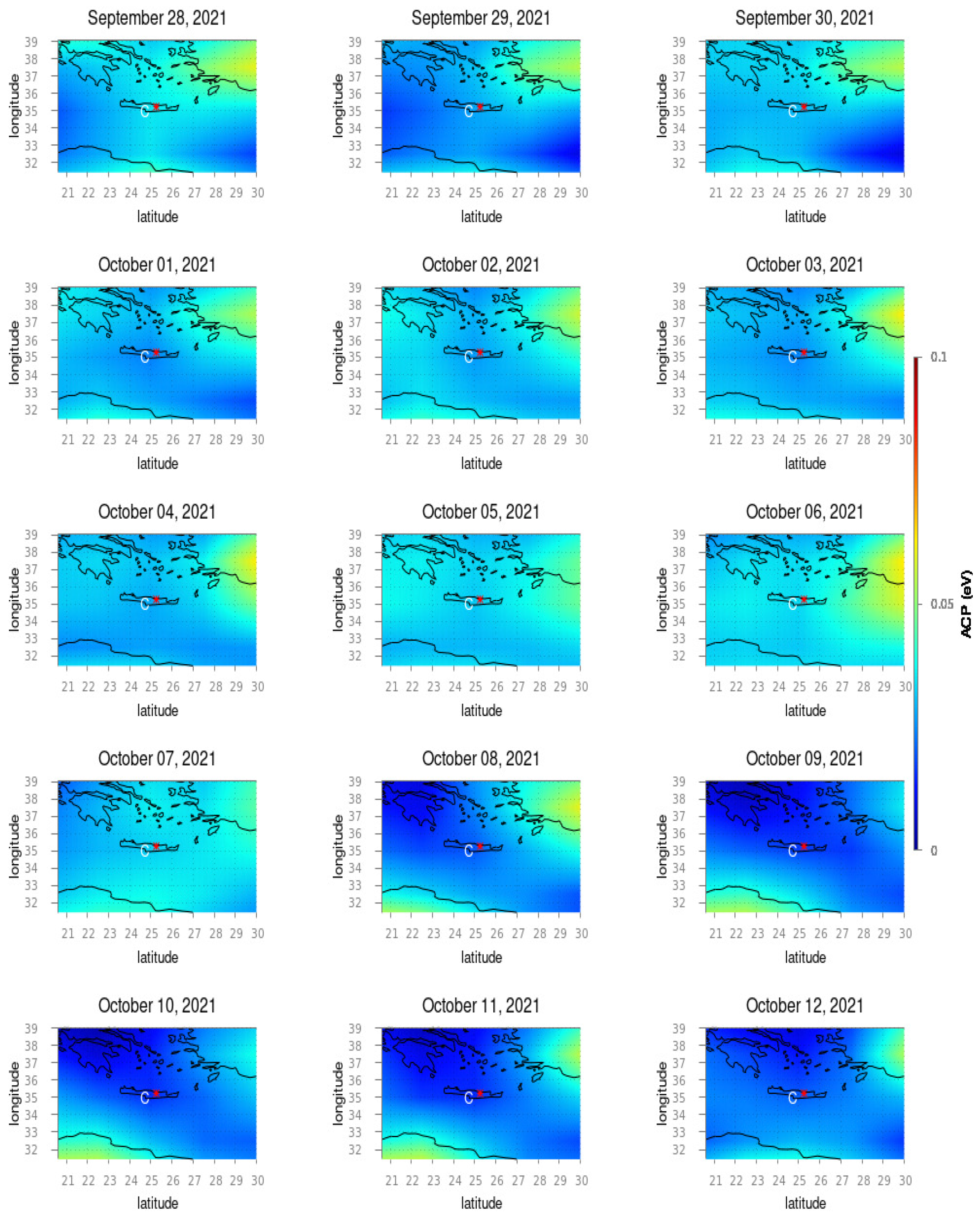
In Figure 6 and Figure 7, we present the spatio-temporal variation in the ACP within the earthquake preparation zone. The ACP value started showing an anomalous increase from 16 September, and the maximum ACP value near the epicenter of the studied earthquake was observed on 21 September. Again, on 26 September, the ACP value increased rapidly near the epicenter. From Figure 7, it was found that during October, the ACP value remained normal, and no rapid increase was observed near the epicenter.
4. Discussion
This work uses space-based observation to present the lower atmospheric thermal anomalies associated with the Crete earthquake that took place on 27 September 2021. We investigated the anomalies in the SHLF, OLR, and ACP by using the NOAA reanalysis data. The spatio-temporal profiles of these parameters were studied around the earthquake occurrence day after the removal of background profiles by choosing a non-seismic period of observation.
- (i)
- It is evident from Figure 2 that the intensification in the SLHF is observed on 23 and 24 September 2021 over the epicenter region. The intensified SLHF shows a longitudinal spread over the earthquake epicenter and migrates towards the southeast direction. After the earthquake, comparatively less intensification is observed from 29 September to 6 October 2021 (Figure 2). For all these days, the anomalies are observed mostly in the north–south direction over the epicenter. This can be attributed to the combined effects of a series of aftershocks of the mainshock of 27 September and a second mainshock that took place on 12 October 2021, south-southeast of Crete island, the epicenter of which was in close vicinity of the first mainshock.
- (ii)
- In contrast to the SLHF, the intensification in the OLR Eddy Field was observed from 18 to 21 September 2021, in two different patches in the northeast and northwest directions of the epicenter, which lie within the earthquake preparation zone (Figure 4). On 23 and 24 September, it became a single intensification over the epicenter, similar to the SLHF variation. After the Crete earthquake, a similar post-earthquake OLR Eddy field enhancement was observed with much less intensity (Figure 5). On 12 September 2021, the Eddy Field again increased in the northern direction of the epicenter, possibly due to the second mainshock mentioned above.
- (iii)
- The ACP variation shows an anomalous increase from 16 September, and the maximum enhancement took place on 21 September 2021 (Figure 6). During this period, the intensification of the ACP is found to be a bit away from the epicenter of the 2021 Crete earthquake. On 26 September, a secondary enhancement was observed near the earthquake epicenter. For the ACP, no such post-earthquake enhancement is observed, in contrast to the SLHF and OLR.
The analysis of very-low-frequency (VLF) sub-ionospheric propagation data received at multiple receivers during the 2021 Crete earthquake shows a moderate shift in electron density variation during the sunrise and sunset terminator times observed on 24, 25, and 27 September 2021 for the ISR-UWA propagation path [36]. Significant changes were not observed during both terminator times for the ISR-GER propagation path. However, for the 12 October earthquake, a significant change in the electron density profile was observed. Furthermore, some intermediate change in the electron density profile was observed on 11 October [36]. In the present study, we also found thermal anomalies during the same time period, which indicates that during the pre-seismic process, the lithospheric perturbations percolate to the troposphere and lower ionosphere through various channels according to the LAIC mechanism. The air ionization creates cluster hydration that releases latent heat and increases the air temperature. According to the LAIC hypothesis, this may create an ion uplift by the formation of an EQ cloud, and that reduces the air conductivity. Thus, the ground–ionosphere potential differences are modulated. This changes the horizontal electric field in the ionosphere, leading to ion drifts, and therefore, the electron and ion concentration may become perturbed over the EQ preparation zone. So, a lithospheric phenomenon can be coupled with ionospheric irregularities, as the LAIC theory prescribes. Our study also found that ACP variation is much weaker for the 2021 Crete earthquake than for the other studied case. It was previously reported that near the oceanic earthquake, the ACP values were lower than those of the land earthquakes. We observed a similar variation from the studied case.
Our manuscript shows that the OLR and SHLF give comparatively clearer indications than the ACP. It needs to be noted the ACP is not a fundamental parameter but is derived from two important parameters, viz., air temperature and relative humidity. It is commonly found that during or prior to seismic activities, the air temperature shows an increment, and the relative humidity experiences a decrease in the profiles. Equation (5) in the manuscript shows that the overall ACP values generally show an increase in nature due to the increase and decrease in air temperature and relative humidity, respectively. As OLR and SLHF are not derived parameters, the variabilities in these parameters are different in comparison to the ACP. Furthermore, for a consistent change in the ACP, one can expect equal proportionate changes in air temperature and relative humidity that can satisfy the equation, which is possibly not always true. Thus, the intensification of ACP patches may have more dynamic characteristics in comparison to the other two parameters in this manuscript.
It is very important to accept that based on the research on the LAIC mechanism, a variety of parameters are involved in each channel of LAIC (chemical, thermal, acoustic, and electromagnetic). It needs to be remembered that the pre-seismic processes, as mentioned in LAIC coupling, are highly nonlinear, anisotropic, and multi-parametric in nature. Refs. [38,41] gave a detailed description of this anisotropy and dependency of multi-parameters. The works on surface deformation characteristics [38,47] before strong earthquakes indicate vital information about the frictional force that leads to generating enhanced thermal profiles around an earthquake’s epicenter that sometimes follow the earthquake fault lines. Furthermore, as the friction-generated heat energy is not very regular during the earthquake preparation process [48,49], the increased energy budget due to friction may not be synchronized with the heat energy originated due to geochemical mechanisms. Therefore, there is always a possibility of breaking this synchronization, and it is difficult to identify any particular thermal anomaly that will temporally dominate every time. This is the same for the other parameters in other channels in LAIC. For example, for the well-known Nepal earthquake in April and May 2015, refs. [14,22] reported the OLR and SLHF separately. It is found that the temporal variation does not show proper synchronization. The OLR intensification shows a maximum anomaly 4 to 5 days before the earthquake, whereas the SLHF shows the maximum anomaly 4 to 5 days before the earthquake. Most interestingly, the same parameter (OLR/SLHF) shows different time frames to show the maximum anomaly before the earthquake. Therefore, this is not a linear problem where one can expect similar outcomes every time. The synchronization of all the parameters in individual channels may not happen every time. The anisotropy in the various parameters may bar achieving uniform directionality. For example, even though the spatio-temporal profile of OLR intensification followed the direction of the Himalayan fault line (east to west), a significant amount of the OLR energy budget also went to the north-to-south direction where there was no such fault line [14]. In the LAIC mechanism, the generation of any anomaly is equally important as the migration of such anomalies for the source location due to the presence of other atmosphere dynamics. Therefore, there is quite a possibility that one cannot expect the most intense anomaly over the epicenter every time. In our case, we experienced similar features for OLR anomalies.
5. Conclusions
During the pre-seismic process, the immediate after-effects are observed over the surface and lower tropospheric regions. In this region, the observed effects are mostly in the form of thermal anomalies, which makes it an important channel in the LAIC mechanism. In this study, we used space-based observations of thermal excitation during pre-seismic processes. The Outgoing Longwave Radiation from the fault lines changes the normal temperature trends and relative humidity near the epicenter, which eventually contributes to the Surface Latent Heat Flux anomaly. So, all of these parameters are considered significant parameters in the LAIC mechanism. In this study, we tried to investigate these parameters for the same earthquake and find the contrasting behavior of the parameters due to the geographic location and the parameter with the most potential for studying the precursory effects. We used parameters like the SLHF anomaly, which is originated from the coagulation of the water molecules to ions, whereas the OLR anomaly is directly emerging thermal waves in the infrared range. On the other hand, the ACP depicts the measure of these variations and the extent of the process criticality during pre-seismic conditions. We found that all these parameters exhibit significant increases 3 to 7 days prior to the mainshock of the earthquake near the epicenter. To date, we have been able to show the changes related to pre-seismic processes. So many significant parameters are associated with the LAIC mechanism’s thermal channel and play various roles in seismogenic conditions. We do not have a clear idea of how this complex interplay is taking place and which are the most significant parameters in this interplay. We must study all possible parameters for different geographic and climatic conditions to understand the entire process. Multi-parametric and multidisciplinary approaches will help us understand the LAIC process, starting from the lower atmosphere to the upper ionosphere. A further approach to coordinate the observed anomaly with the ionospheric and magnetospheric perturbations using a multidimensional approach will help us to understand the entire LAIC process. These new approaches to solving the unanswered question of the LAIC mechanism will be studied in the future and will be published elsewhere.
Author Contributions
Conceptualization, S.G., S.S., S.M.P. and M.H.; methodology, S.G. and S.S.; software, S.G., S.S. and S.K.M.; validation, S.G., S.S. and S.M.P.; formal analysis, S.G.; investigation, S.G., S.S. and S.M.P.; resources, S.G. and S.S.; data curation, S.G.; writing—original draft preparation, S.G.; writing—review and editing, S.S., S.M.P. and M.H.; visualization, S.S. and S.M.P.; supervision, S.S., S.M.P. and M.H.; project administration, S.S. All authors have read and agreed to the published version of the manuscript.
Funding
The authors have not received any external funding for this research.
Data Availability Statement
The data are freely available in the NOAA Reanalysis repository https://psl.noaa.gov/data/gridded/data.ncep.reanalysis.html (accessed on 26 April 2023).
Acknowledgments
The authors acknowledge the NOAA for providing satellite data.
Conflicts of Interest
Author Masashi Hayakawa was employed by the company Hayakawa Institute of Seismo-Electromagnetics Co., Ltd. The remaining authors declare that the research was conducted in the absence of any commercial or financial relationships that could be construed as a potential conflict of interest.
References
- Pulinets, S.; Boyarchuk, K. Ionospheric Precursors of Earthquakes; Springer: Berlin/Heidelberg, Germany; New York, NY, USA, 2004; ISBN 3. [Google Scholar] [CrossRef]
- Molchanov, O.A.; Hayakawa, M. Seismo Electromagnetics and Related Phenomena: History and Latest Results; TERRAP: Tokyo, Japan, 2008; 189p. [Google Scholar]
- Ouzounov, D.; Pulinets, S.; Hattori, K.; Taylor, P. (Eds.) Pre-Earthquake Processes: A Multidisciplinary Approach to Earthquake Prediction Studies; AGU Geophysical Monograph; Wiley: Hoboken, NJ, USA, 2018; Volume 234, 365p. [Google Scholar]
- Nayak, K.; López-Urías, C.; Romero-Andrade, R.; Sharma, G.; Guzmán-Acevedo, G.M.; Trejo-Soto, M.E. Ionospheric Total Electron Content (TEC) Anomalies as Earthquake Precursors: Unveiling the Geophysical Connection Leading to the 2023 Moroccan 6.8 Mw Earthquake. Geosciences 2023, 13, 319. [Google Scholar] [CrossRef]
- Sharma, G.; Saikia, P.; Walia, D.; Banerjee, P.; Raju, P.L.N. TEC anomalies assessment for earthquakes precursors in North-Eastern India and adjoining region using GPS data acquired during 2012–2018. Quat. Int. 2021, 575, 120–129. [Google Scholar] [CrossRef]
- Molchanov, O.A. Lithosphere-Atmosphere-Ionosphere Coupling due to Seismicity. Electromagn. Phenom. Assoc. Earthq. 2009, 255–279. [Google Scholar]
- Pulinets, S.; Ouzonov, D. Lithosphere-Atmosphere-Ionosphere Coupling (LAIC) model-An unified concept for earthquake precursors validation. J. Asian Earth Sci. 2011, 41, 371–382. [Google Scholar] [CrossRef]
- Omori, Y.; Yasuoka, Y.; Nagahama, H.; Kawada, Y.; Ishikawa, T.; Tokonami, S.; Shinogi, M. Anomalous radon emanation linked to preseismic electromagnetic phenomena. Nat. Hazards Earth Syst. Sci. 2007, 7, 629–635. [Google Scholar] [CrossRef]
- Klimenko, M.V.; Klimenko, V.V.; Zakharenkova, I.E.; Pulinets, S.A.; Zhao, B.; Tsidilina, M.N. Formation mechanism of great positive TEC disturbances prior to Wenchuan earthquake on May 12, 2008. Adv. Space Res. 2011, 48, 488–499. [Google Scholar] [CrossRef]
- Asano, T.; Hayakawa, M. On the tempo-spatial evolution of the lower ionospheric perturbation for the 2016 Kumamoto earthquakes from comparisons of VLF propagation data observed at multiple stations with wave-hop theoretical computations. Open J. Earthq. Res. (OJER) 2018, 7, 161–185. [Google Scholar] [CrossRef]
- Biswas, S.; Kundu, S.; Chowdhury, S.; Ghosh, S.; Yang, S.; Hayakawa, M.; Chakraborty, S.; Chakrabarti, S.; Sasmal, S. Contaminated effect of geomagnetic storm on pre-seismic atmospheric and ionospheric anomalies during imphal earthquake. Open J. Earthq. Res. (OJER) 2020, 9, 383–402. [Google Scholar] [CrossRef]
- Chakrabarti, S.K.; Sasmal, S.; Chakrabarti, S. Ionospheric anomaly due to seismic activities-II: Possible evidence from D-layer preparation and disappearance times. Nat. Hazards Earth Syst. Sci. 2010, 10, 1751–1757. [Google Scholar] [CrossRef]
- Chakraborty, S.; Sasmal, S.; Basak, T.; Ghosh, S.; Palit, S.; Chakrabarti, S.K.; Ray, S. Numerical modeling of possible lower ionospheric anomalies associated with Nepal earthquake in May, 2015. Adv. Space Res. 2017, 60, 1787–1796. [Google Scholar] [CrossRef]
- Chakraborty, S.; Sasmal, S.; Chakrabarti, S.K.; Bhattacharya, A. Observational signatures of unusual outgoing longwave radiation (OLR) and atmospheric gravity waves (AGW) as precursory effects of May 2015 Nepal earthquakes. J. Geodyn. 2018, 113, 43–51. [Google Scholar] [CrossRef]
- Ghosh, S.; Sasmal, S.; Midya, S.; Chakrabarti, S. Unusual Change in Critical Frequency of F2 Layer during and Prior to Earthquakes. J. Open Earthq. Res. (OJER) 2017, 6, 191–203. [Google Scholar] [CrossRef]
- Ghosh, S.; Chakraborty, S.; Sasmal, S.; Basak, T.; Chakrabarti, S.K.; Samanta, A. Comparative study of the possible lower ionospheric anomalies in Very Low Frequency (VLF) signal during Honshu, 2011 and Nepal, 2015 earthquakes. Geomat. Nat. Hazards Risk 2019, 10, 1596–1612. [Google Scholar] [CrossRef]
- Hayakawa, M.; Molchanov, O.A.; Ondoh, T.; Kawai, E. Anomalies in the sub-ionospheric VLF signals for the 1995 Hyogo-ken Nanbu earthquake. J. Phys. Earth 1996, 44, 413–418. [Google Scholar] [CrossRef]
- Hayakawa, M.; Molchanov, O.A.; Ondoh, T.; Kawai, E. The precursory signature effect of the Kobe earthquake on VLF subionospheric signals. J. Comm. Res. Lab. Tokyo 1996, 43, 169–180. [Google Scholar]
- Hayakawa, M.; Potirakis, S.M.; Saito, Y. Possible relation of air ion density anomalies with earthquakes and the associated precursory ionospheric perturbations: An analysis in terms of criticality. Int. J. Electron. Appl. Res. 2018, 5, 56–75. [Google Scholar] [CrossRef]
- Sasmal, S.; Chakrabarti, S.K. Ionosperic anomaly due to seismic activities—Part 1: Calibration of the VLF signal of VTX 18.2 kHz station from Kolkata and deviation during seismic events. Nat. Hazards Earth Syst. Sci. 2009, 9, 1403–1408. [Google Scholar] [CrossRef]
- Sasmal, S.; Chakrabarti, S.K.; Ray, S. Unusual behavior of Very Low Frequency signal during the earthquake at Honshu/Japan on 11 March, 2011. Indian J. Phys. 2014, 88, 1013–1019. [Google Scholar] [CrossRef]
- Ghosh, S.; Chowdhury, S.; Kundu, S.; Sasmal, S.; Politis, D.Z.; Potirakis, S.M.; Hayakawa, M.; Chakraborty, S.; Chakrabarti, S.K. Unusual Surface Latent Heat Flux Variations and Their Critical Dynamics Revealed before Strong Earthquakes. Entropy 2022, 24, 23. [Google Scholar] [CrossRef]
- Ghosh, S.; Sasmal, S.; Naja, M.; Potirakis, S.; Hayakawa, M. Study of aerosol anomaly associated with large earthquakes (M > 6). Adv. Space Res. 2022, 71, 129–143. [Google Scholar] [CrossRef]
- Pulinets, S.; Ouzounov, D.; Karelin, A.; Davidenko, D. Physical Bases of the Generation of Short Term Earthquake Precursors: A Complex Model of Ionization Induced Geophysical Processes in the Lithosphere–Atmosphere–Ionosphere–Magnetosphere System. Geomagn. Aeron. 2015, 55, 521–538. [Google Scholar] [CrossRef]
- Kondepudi, D.; Prigogine, I. Modern Thermodynamics: From Heat Engines to Dissipative Structures; Wiley: Chichester, UK, 1998. [Google Scholar]
- Pulinets, S.A.; Ouzounov, D.; Karelin, A.V.; Boyarchuk, K.A.; Pokhmelnykh, L.A. The physical nature of the thermal anomalies observed before strong earthquakes. Phys. Chem. Earth 2006, 31, 143–153. [Google Scholar] [CrossRef]
- Gorny, V.I.; Salman, A.G.; Tronin, A.A.; Shilin, B.V. The Earth’s outgoing IR radiation as an indicator of seismic activity. Proc. Acad. Sci. USSR 1988, 301, 67–69. [Google Scholar]
- Ouzounov, D.; Freund, F. Mid-infrared emission prior to strong earthquakes analyzed by remote sensing data. Adv. Space Res. 2004, 33, 268–273. [Google Scholar] [CrossRef]
- Qiang, Z.J.; Xu, X.D.; Dian, C.G. Abnormal infrared thermal satellite-forewarning of earthquakes. Chin. Sci. Bull. 1990, 35, 1324–1327. [Google Scholar]
- Saraf, A.K.; Choudhury, S. Satellite detects surface thermal anomalies associated with the Algerian earthquakes of May 2003. Int. J. Remote Sens. 2004, 26, 2705–2713. [Google Scholar] [CrossRef]
- Tronin, A.A. Satellite thermal survey—A new tool for the study of seismo active regions. Int. J. Remote Sens. 1996, 41, 1439–1455. [Google Scholar] [CrossRef]
- Tronin, A.A.; Hayakawa, M.; Molchanov, O.A. Thermal IR satellite data application for earthquake research in Japan and China. J. Geodyn. 2002, 33, 519–534. [Google Scholar] [CrossRef]
- Xu, X.; Qiang, Z.; Dian, C. Thermal infrared image of Meteosat and prediction of impending earthquake–conclusion of studying thermal infrared image before Lanhang-Genma earthquake occurring. Remote Sens. Environ. 1991, 6, 261–266. [Google Scholar]
- Pulinets, S.; Ouzounov, D.; Karelin, A.; Davidenko, D. Lithosphere-Atmosphere-Ionosphere-Magnetosphere Coupling—A Concept for Pre-Earthquake Signals Generation. In Pre-Earthquake Processes: A Multidisciplinary Approach to Earthquake Prediction Studies; Ouzounov, D., Pulinets, S., Hattori, K., Taylor, P., Eds.; AGU/Wiley: Washington, DC, USA, 2018; pp. 77–98. [Google Scholar]
- Pulinets, S.; Budnikov, P. Atmosphere Critical Processes Sensing with ACP. Atmosphere 2022, 13, 1920. [Google Scholar] [CrossRef]
- Politis, D.Z.; Potirakis, S.M.; Sasmal, S.; Malkotsis, F.; Dimakos, D.; Hayakawa, M. Possible Pre-Seismic Indications Prior to Strong Earthquakes That Occurred in Southeastern Mediterranean as Observed Simultaneously by Three VLF/LF Stations Installed in Athens(Greece). Atmosphere 2023, 14, 673. [Google Scholar] [CrossRef]
- Biswas, S.; Chowdhury, S.; Sasmal, S.; Politis, D.Z.; Potirakis, S.M.; Hayakawa, M. Numerical modelling of sub-ionospheric Very Low Frequency radio signal anomalies during the Samos (Greece) earthquake (M = 6.9) on October 30, 2020. Adv. Space Res. 2022, 70, 1453–1471. [Google Scholar] [CrossRef]
- Chowdhury, S.; Kundu, S.; Ghosh, S.; Hayakawa, M.; Schekotov, A.; Potirakis, S.M.; Chakrabarti, S.K.; Sasmal, S. Direct and indirect evidence of pre-seismic electromagnetic emissions associated with two large earthquakes in Japan. Nat. Hazards 2022, 112, 2403–2432. [Google Scholar] [CrossRef]
- Hayakawa, M.; Schekotov, A.; Izutsu, J.; Yang, S.-S.; Solovieva, M.; Hobara, Y. Multi-Parameter Observations of Seismogenic Phenomena Related to the Tokyo Earthquake (M = 5.9) on 7 October 2021. Geosciences 2022, 12, 265. [Google Scholar] [CrossRef]
- Kundu, S.; Chowdhury, S.; Ghosh, S.; Sasmal, S.; Politis, D.Z.; Potirakis, S.M.; Yang, S.S.; Chakrabarti, S.K.; Hayakawa, M. Seismogenic Anomalies in Atmospheric Gravity Waves as Observed from SABER/TIMED Satellite during Large Earthquakes. J. Sens. 2022, 2022, 3201104. [Google Scholar] [CrossRef]
- Sasmal, S.; Chowdhury, S.; Kundu, S.; Politis, D.Z.; Potirakis, S.M.; Balasis, G.; Hayakawa, M.; Chakrabarti, S.K. Pre-Seismic Irregularities during the 2020 Samos (Greece) Earthquake (M = 6.9) as Investigated from Multi-Parameter Approach by Ground and Space-Based Techniques. Atmosphere 2021, 12, 1059. [Google Scholar] [CrossRef]
- Kang, C.; Liu, D. The applicability of satellite remote sensing in monitoring earthquake. Sci. Surv. Mapp. 2001, 26, 46–48. [Google Scholar]
- Liu, D.; Peng, K.; Liu, W.; Li, L.; Hou, J. Thermal omens before earthquake. Acta Seismol. Sin. 1999, 12, 710–715. [Google Scholar] [CrossRef]
- Liu, D. Anomalies analyses on satellite remote sensing OLR before Jiji earthquake of Taiwan Province. Geo-Inf. Sci. 2000, 2, 33–36. [Google Scholar]
- Xiong, P.; Shen, X.H.; Bi, Y.X.; Kang, C.L.; Chen, L.Z.; Jing, F.; Chen, Y. Study of outgoing longwave radiation anomalies associated with Haiti earthquake. Nat. Hazards Earth Syst. Sci. 2010, 10, 2169–2178. [Google Scholar] [CrossRef]
- Boyarchuk, K.A.; Karelin, A.V.; Shirokov, R.V. Bazovaya Model’ Kinetiki Ionizirovannoi Atmosfery (The Reference Model of Ionized Atmospheric Kinetics); VNIIEM: Moscow, Russia, 2006. [Google Scholar]
- Yang, S.S.; Potirakis, S.M.; Sasmal, S.; Hayakawa, M. Natural Time Analysis of Global Navigation Satellite System Surface Deformation: The Case of the 2016 Kumamoto Earthquakes. Entropy 2020, 22, 674. [Google Scholar] [CrossRef]
- Aubry, J.; Passelègue, F.X.; Deldicque, D.; Girault, F.; Marty, S.; Lahfid, A.; Bhat, H.S.; Escartin, J.; Schubnel, A. Frictional Heating Processes and Energy BudgetDuring Laboratory Earthquakes. Geophys. Res. Lett. 2018, 12, 274. [Google Scholar]
- Coffey, J.L.; Savage, H.M.; Polissar, P.J. Estimates of earthquake temperature rise, frictional energy, and implications to earthquake energy budgets. Seismica 2023, 2. [Google Scholar] [CrossRef]
Figure 1.
The location of the earthquake epicenter (red circle), the earthquake preparation zone (black circle), and the local earthquake fault lines for the Crete, Greece, earthquake.
Figure 1.
The location of the earthquake epicenter (red circle), the earthquake preparation zone (black circle), and the local earthquake fault lines for the Crete, Greece, earthquake.
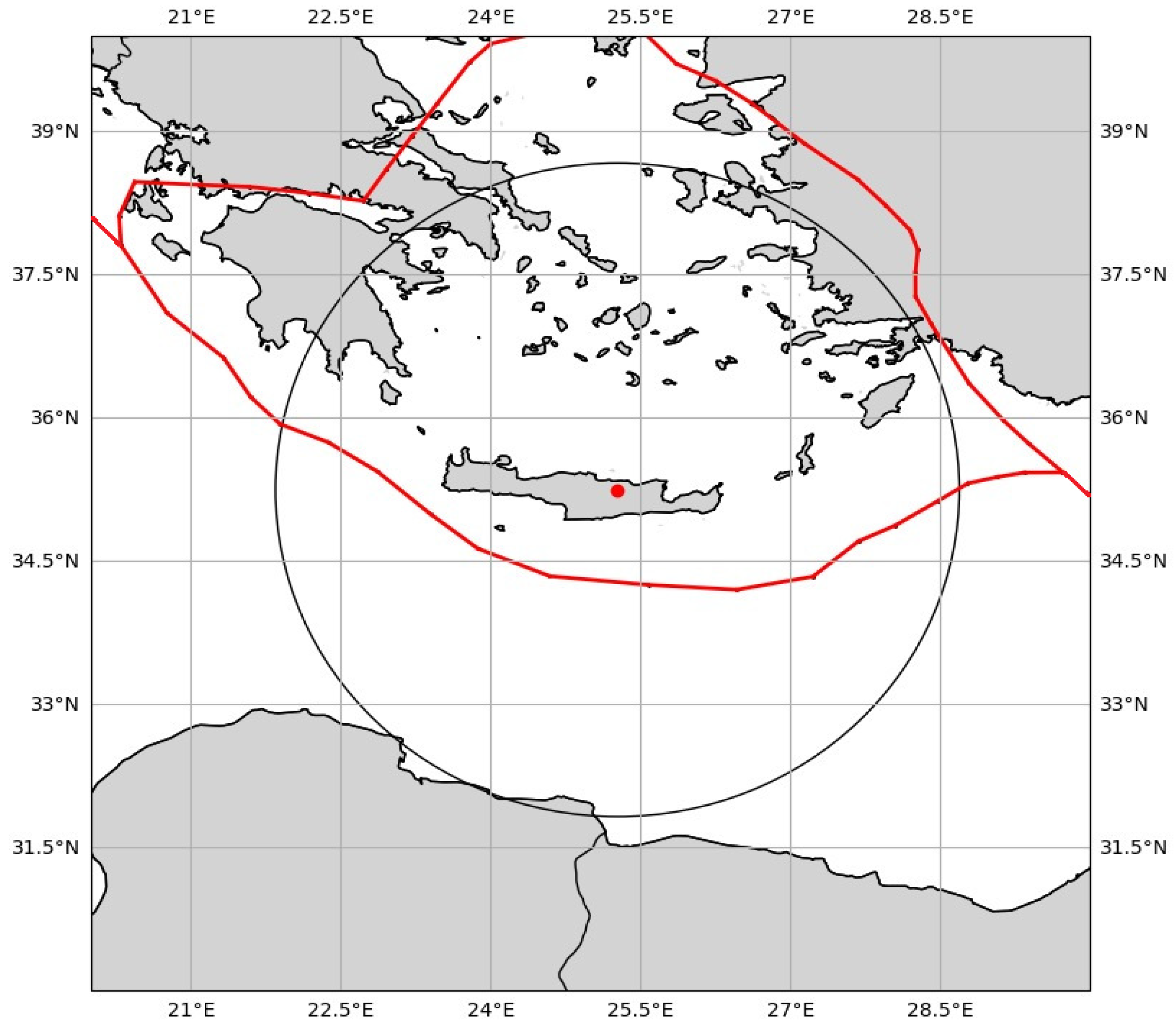
Figure 2.
Variation in the SLHF anomaly from 13 to 27 September 2021 for the Crete earthquake. Along the X and Y axes, we present the geographic longitude and latitude, respectively. The black outlines are the country border, and the red dot marks the epicenter of the Crete earthquake, also denoted by the letter “C”.

Figure 3.
SLHF anomaly variation from 28 September to 12 October 2021. The figure format follows the format of Figure 2. The black outlines are the country border, and the red dot marks the epicenter of the Crete earthquake, also denoted by the letter “C”.
Figure 3.
SLHF anomaly variation from 28 September to 12 October 2021. The figure format follows the format of Figure 2. The black outlines are the country border, and the red dot marks the epicenter of the Crete earthquake, also denoted by the letter “C”.

Figure 4.
Eddy Field OLR variations around the Crete earthquake epicenter during 13–27 September 2021 with a spatial span of latitudes 30° N to 39° N and longitudes 20° E to 30° E. The red dot and the letter “C” indicate the epicenter of the Crete earthquake. The country boundaries are indicated by black lines. The color bar represents the intensity of the mean Eddy Field in W/m2.

Figure 5.
Same as Figure 4 for 28 September to 12 October 2021. The black outlines are the country border, and the red dot marks the epicenter of the Crete earthquake, also denoted by the letter “C”.
Figure 5.
Same as Figure 4 for 28 September to 12 October 2021. The black outlines are the country border, and the red dot marks the epicenter of the Crete earthquake, also denoted by the letter “C”.

Figure 6.
ACP distribution around the epicenter of the Crete earthquake from 28 September to 12 October 2021. The black outlines are the country border, and the red dot marks the epicenter of the Crete earthquake, also denoted by the letter “C”.
Figure 6.
ACP distribution around the epicenter of the Crete earthquake from 28 September to 12 October 2021. The black outlines are the country border, and the red dot marks the epicenter of the Crete earthquake, also denoted by the letter “C”.
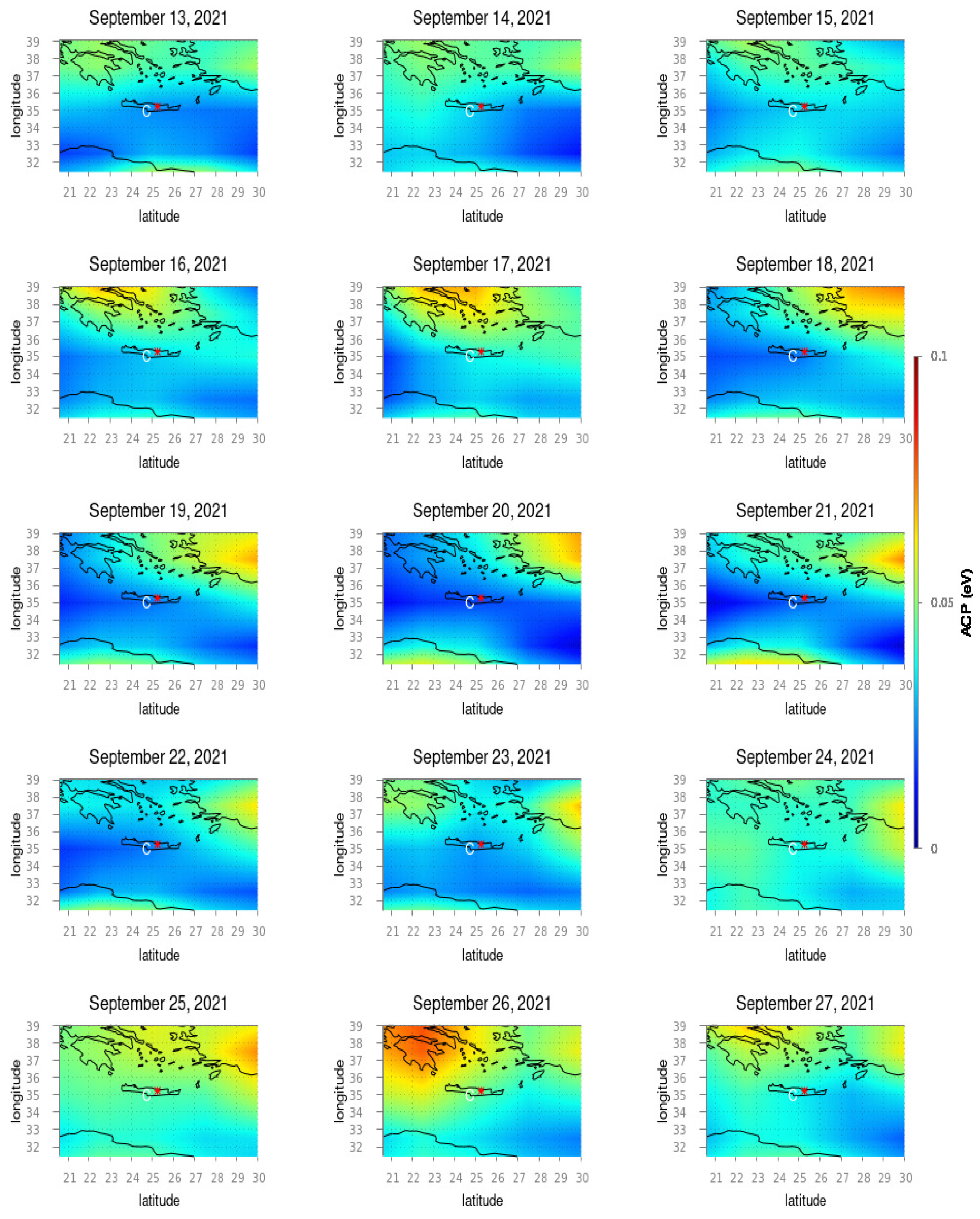
Figure 7.
Same as Figure 6 for 28 September to 12 October 2021. The black outlines are the country border, and the red dot marks the epicenter of the Crete earthquake, also denoted by the letter “C”.
Figure 7.
Same as Figure 6 for 28 September to 12 October 2021. The black outlines are the country border, and the red dot marks the epicenter of the Crete earthquake, also denoted by the letter “C”.

Table 1.
Earthquake details.
| Earthquake | Location of Epicenter | Magnitude () | Depth (km) | Date and Time (UT) | Radius of Preparation Zone (km) |
|---|---|---|---|---|---|
| Crete Earthquake | 35.244° N 25.27° E | 6 | 6 | 27 September 2021 06:17:21 | 380.189 |
Disclaimer/Publisher’s Note: The statements, opinions and data contained in all publications are solely those of the individual author(s) and contributor(s) and not of MDPI and/or the editor(s). MDPI and/or the editor(s) disclaim responsibility for any injury to people or property resulting from any ideas, methods, instructions or products referred to in the content. |
© 2024 by the authors. Licensee MDPI, Basel, Switzerland. This article is an open access article distributed under the terms and conditions of the Creative Commons Attribution (CC BY) license (https://creativecommons.org/licenses/by/4.0/).
Share and Cite
MDPI and ACS Style
Ghosh, S.; Sasmal, S.; Maity, S.K.; Potirakis, S.M.; Hayakawa, M. Thermal Anomalies Observed during the Crete Earthquake on 27 September 2021. Geosciences 2024, 14, 73. https://doi.org/10.3390/geosciences14030073
AMA Style
Ghosh S, Sasmal S, Maity SK, Potirakis SM, Hayakawa M. Thermal Anomalies Observed during the Crete Earthquake on 27 September 2021. Geosciences. 2024; 14(3):73. https://doi.org/10.3390/geosciences14030073
Chicago/Turabian StyleGhosh, Soujan, Sudipta Sasmal, Sovan K. Maity, Stelios M. Potirakis, and Masashi Hayakawa. 2024. "Thermal Anomalies Observed during the Crete Earthquake on 27 September 2021" Geosciences 14, no. 3: 73. https://doi.org/10.3390/geosciences14030073
Note that from the first issue of 2016, this journal uses article numbers instead of page numbers. See further details here.