An Inversion Method for Surrounding Rock Parameters of Tunnels Based on a Probabilistic Baseline Model under a Constructional Environment

Abstract

The uncertainty of surrounding rock parameters varies due to changes in the boundary conditions of the tunnel model, and no suitable method to ensure that the updated parameters of the finite element model (FEM) are applicable throughout the constructional environment. To address this issue, a probabilistic baseline model method was introduced to invert the rock parameters and obtain values suitable for the complete constructional environment. First, the probabilistic statistical theory was applied to statistically analyze the measurement data from tunnels under different constructional environments, which provides insight into the variation in rock parameters. Then, an objective optimization function based on a genetic algorithm (GA) was constructed to optimize the accuracy by minimizing the error between the measurement data and the simulation data. Next, a Kriging model was built that utilized Young’s modulus and cohesion as updated parameters. This approach contributes to overcoming the inefficiency of multi-objective optimization computations. By using the Kriging model, optimal values for the rock parameters were obtained. Finally, the effectiveness and applicability of the proposed method were validated by comparing the measured data with the updated model data under different constructional environments.

1. Introduction

The geological environment of tunnel structures presents a high degree of complexity and the physical-mechanical parameters of the surrounding rock exhibit non-linear, non-continuous and non-uniform behavior. The complexity is further exacerbated by the construction environment, which further increases the uncertainties. Accurate determination of rock parameters plays a crucial role in assessing the stability of the structure and preventing engineering disasters. In simulating the actual geological structure and accurately describing the structural behaviors, it is essential to obtain reliable and precise surrounding rock parameters. The challenges of accurately modeling such complex engineering materials have been highlighted in various studies [1,2]. The researchers emphasized the need for improved models and methods to capture and represent the complexities of the surrounding rock. In recent years, several researchers have tackled this issue and proposed different approaches to obtain accurate surrounding rock parameters [3,4,5]. These studies recognize the importance of considering specific geological conditions and emphasize the use of advanced techniques to optimize the estimation of rock parameters [6]. By considering these advancements and the complexities of the geological environment, researchers aim to develop more accurate and reliable models that can better describe the behavior of the surrounding rock in tunnel structures.

Currently, in situ or laboratory rock testing to obtain physical and mechanical parameters of rock masses is the most common method. Researchers such as Aida Erfanian Pour and Mohammad Reza Majedi have conducted laboratory experiments on rocks to analyze fracture parameters during rock failure and extract physical and mechanical strength. They showed that parameters obtained this way effectively modify constructed models [7,8]. However, compared to traditional indoor or field experiments, the application of inversion methods based on field monitoring data is a more feasible, efficient and economical way to obtain rock parameters [9,10,11]. Researchers have extensively investigated inversion methods for estimating structural parameters from field monitoring data and the findings are remarkable [12,13]. In the field of underground engineering, parameter inversion methods can be classified into three groups: analytical methods, numerical methods and machine learning methods [14]. However, analytical and numerical methods are limited in dealing with complex geometric shapes and boundary conditions and often require significant computation time. To obtain more accurate input parameters, the numerical analysis problem is converted into an optimization problem. The discrepancy between the machine learning calculations and the actual measured displacements is taken as the optimization objective [15,16,17]. Consequently, more researchers are attempting to invert structural rock parameters through objective optimization, and various optimization methods have been applied.

The prevailing back analyses in current geotechnical practice can be classified into two categories: the deterministic approach and the probabilistic approach [18,19]. In the deterministic back analysis, the uncertainties of the input parameters and solution models are ignored. Back analysis aims to obtain a single set of geotechnical parameters that matches the prediction with the observation [20]. However, when this method is applied to structural parameter inversion, it often relies on deterministic actual cumulative monitoring values, neglecting uncertainties, such as measurement errors and spatial variability of parameters in the building environment. As a result, the updated surrounding rock parameters may not be suitable for the entire structural environment of the model. On the other hand, probabilistic back analysis explicitly considers the uncertainties of the solution models and input parameters. It allows for updating these uncertain variables in numerous combinations, each with different relative probabilities, to match the prediction with the observation [21]. In the presence of uncertainties, probabilistic back analysis offers several advantages over deterministic back analysis, making it the preferred approach for performing back analysis in past decades [22,23,24]. At present, the common probabilistic inverse analysis methods include the least square method, maximum likelihood method, extended Kalman filtering technology and Bayesian method [25]. Compared with other methods, the Bayesian method has the characteristics of being stable and highly efficient in dealing with uncertainty, which is why it is widely used in geotechnical engineering. However, many uncertain factors exist in geotechnical engineering, which leads to incomplete consideration of the parameter inversion process of the traditional Bayesian method. To solve this problem, Haotian Zheng and Michael Mooney proposed a surrogate-based Bayesian approach to update the ground parameters. This method can consider the time-series observations of multiple types of measurements are used to form the likelihood function. The proposed method was a reasonable solution for the selection of uncertainties in the process of back analysis of geotechnical parameters [26]. The method has played a supporting role. Therefore, many scholars have tried to select different methods to study the complex uncertainty of geotechnical engineering.

With the development of large datasets and information technology, researchers are attempting to address the issue of uncertainty in parameter inversion by adopting novel monitoring tools and analysis techniques [27,28]. Specifically, for structural uncertainty arising from measurement errors and spatial effects during tunnel construction, an analytical framework for tunnel model inversion has been established. This framework combines various numerical models with new optimization algorithms. The results have demonstrated the valuable reference significance of the inversion parameters, leading to continuous improvement of the new algorithm. This approach offers a novel solution to the uncertainty problem in the structural inversion process [29,30,31]. However, when probabilistic inversion methods for tunnel structure parameters are employed, the computational inefficiency of large-scale finite elements and the redundancy of monitoring data decrease inversion efficiency. Hence, to study the uncertainty of structural parameters from a probabilistic statistical perspective, it is necessary to address the challenge of the computational time cost.

In order to address the computational inefficiency of uncertainty inversion methods, researchers have proposed the use of computationally inexpensive meta-modeling as an alternative to exact fitness evaluations. Metamodeling minimizes the number of expensive fitness evaluations by training metamodels on existing evaluated individuals; thus, it directs the search for promising solutions. Several studies have explored the use of metamodels in the inversion process of structural parameters to improve computational efficiency [32,33,34,35]. The application of meta modeling, such as the two-step method proposed by Liu, which combines the Kriging predictor with component Modal synthesis (CMS) technology, ensures the successful implementation of finite element updating for large structures. Additionally, cluster analysis has been introduced into random finite element updating, resulting in the generation of a finite element probability baseline model for bridges and the verification of the proposed method [36,37]. In addition, a Bayesian model revision method based on proxy models has been proposed. It updates uncertain geotechnical parameters in the construction process through a step-by-step Bayesian updating process. The results show that the updated deformation prediction results of surface, subsurface and structures are consistent with the field measurement results [38]. In the field of civil engineering, machine learning algorithms have also been applied to improve computational efficiency. The current main objective of the model revision is to obtain a baseline model that accurately and efficiently represents the physical state changes of structures [39]. With the development of new equipment and the integration of multiple data sources, the monitoring information of civil engineering structures has become more comprehensive. These advances have diversified the methods used to obtain structural baseline models [40]. These studies highlight the application of metamodeling and machine learning in civil engineering to enhance the computational efficiency of inversion methods and to improve the accuracy and effectiveness of structural parameter analysis and crack detection.

In the previous structural parameter inversion, although some scholars have studied structural uncertainty, there is a lack of research on the probabilistic uncertainty of mechanical parameters in the surrounding rock of tunnels under constructional conditions. Most studies have considered these parameters deterministic and have not investigated their probabilistic characteristics. Therefore, unlike other studies, we introduce a probabilistic baseline modeling method to investigate the inversion of surrounding rock physical and mechanical parameters under a constructional environment, and we combine the kriging predictor as a model to deal with the inefficiency of the multi-objective optimization process. Finally, we compare the measurement data and provide an implementation case to verify the superior performance of this method.

2. Theory of the Proposed Method

2.1. Basic Idea of Tunnel Parameter Inversion Based on Probabilistic Baseline Modeling

The geological conditions in the vicinity of tunnels can be highly intricate and varied. Even if the overall level of the surrounding rock is similar, there can still be variations in geological features, such as interbedding and joints. These variations can have a significant effect on the physical and mechanical parameters of the surrounding rock; thus, they are uncertain and have no definite value. However, due to the uncertain nature of these parameters, their estimated values can be considered random variables that follow certain probability distributions. The inherent uncertainty and variability in estimating these parameters is recognized from a probabilistic perspective. This concept is confirmed by the work of Sun and Betti, who emphasized the need to consider the physical and mechanical parameters of the surrounding rock as random variables rather than deterministic quantities [41]. This probabilistic framework allows for a more comprehensive and realistic representation of the uncertainties associated with the physical and mechanical properties of the rock surrounding a tunnel.

$\theta ={[{\theta }_1,{\theta }_2,\cdots ,{\theta }_v,\cdots ,{\theta }_N]}_{m\times N}$ is a set of sample estimates of the parameters of tunnel rock updating, where $m$ and $N$ are the total number of parameter samples and the number of updating parameters respective. In addition, each element of the ${\mathbf{\theta }}_v={\left\{{\mathbf{\theta }}_1,{\mathbf{\theta }}_2,\cdots ,{\mathbf{\theta }}_m\right\}}^T\left(v=1,2,\cdots N\right)$ set is defined as a vector. According to the statistical theory, the mean $\overline{\theta }$ and covariance $\mathit{Cov}\left(\theta \right)$ of the samples of the updating parameters are defined as the following vectors and matrices, respectively:

$$\overline{\theta }=\left\{E\left(\theta \right)\right\}=\frac{1}{N}{\displaystyle \sum _{v=1}^N{\theta }_v}$$

(1)

$$\left[\mathit{Cov}\left(\theta \right)\right]=\frac{1}{N}{\displaystyle \sum _{v=1}^N\left({\theta }_v-\overline{\theta }\right)}{\left({\theta }_v-\overline{\theta }\right)}^T$$

(2)

where $E\left(\theta \right)$ is mathematical expectation operator; $Cov\left(\theta \right)$ is the covariance operator.

Since the updating parameter is a random variable, and the structural deformation results obtained from the actual monitoring data are also random variables due to the equipment and human measurements, the set of sample estimates $Z\left(\theta \right)$ of the displacements measured during tunnel construction is defined as:

$$Z\left(\theta \right)=\left[Z\left({\theta }_1\right),Z\left({\theta }_2\right),\cdots ,Z\left({\theta }_v\right),\cdots ,Z\left({\theta }_N\right)\right]$$

(3)

Each of the following expansions according to Taylor’s first order yields $Z\left(\theta \right)$:

$$Z\left({\theta }_v\right)=Z\left(\overline{\theta }\right)+G\left(\overline{\theta }\right)\left({\theta }_v-\overline{\theta }\right)$$

(4)

where $G\left(\theta \right)$ is the deviation of $Z\left(\theta \right)$ and $\overline{\theta }$, i.e., the sensitivity matrix.

The sample mean of a set $Z\left(\theta \right)$ can be approximated by the following equations:

$$\begin{array}{ll}\left\{\mathrm{E}\left(Z\left(\theta \right)\right)\right\}& =\frac{1}{N}{\displaystyle \sum _{i=1}^N\left(Z\left(\overline{\theta }\right)+G\left(\theta \right)\right)}\left({\theta }_v-\overline{\theta }\right)\\ & =Z\left(\overline{\theta }\right)+G\left(\theta \right)\left(\frac{1}{N}{\displaystyle \sum _{v=1}^N{\theta }_v-\overline{\theta }}\right)=Z\left(\overline{\theta }\right)\end{array}$$

(5)

The covariance matrix of $Z\left(\theta \right)$ is defined as:

$$\begin{array}{ll}\left[\mathit{Cov}\left(Z\left(\theta \right)\right)\right]& =\frac{1}{N}{\displaystyle \sum _{v=1}^N\left(Z\left({\theta }_v\right)-Z\left(\overline{\theta }\right)\right)}{\left(Z\left({\theta }_v\right)-Z\left(\overline{\theta }\right)\right)}^T\\ & =\frac{1}{N}{\displaystyle \sum _{v=1}^N\left(G\left(\overline{\theta }\right)\left({\theta }_{\mathrm{v}}-\overline{\theta }\right)\right)}{\left(G\left(\overline{\theta }\right)\left({\theta }_{\mathrm{v}}-\overline{\theta }\right)\right)}^T\\ & =G\left(\overline{\theta }\right)\left[Cov\left(\theta \right)\right]G{\left(\overline{\theta }\right)}^T\end{array}$$

(6)

The above equations show the mean $\overline{\theta }$ and variance $Cov\left(\theta \right)$ of the rock mass parameters of the tunnel if the measured data are taken in random samples. It is possible to invert the rock mass parameters from the perspective of probabilistic statistics by minimizing the error between the FEM calculation results and the measurement data, and then the probabilistic baseline model of the tunnel is generated.

2.2. Sensitivity Analysis of the Tunneling Model Based on Complex Perturbations

In Equation (3), we know that the sensitivity matrix $G\left(\overline{\theta }\right)$ is based on the deviation from $Z\left(\theta \right)$ and $\overline{\theta }$. The accuracy of the sensitivity matrix plays an important role in FEM updating [42]. By adopting a sensitivity matrix calculation method based on complex perturbations [43,44], the sensitivity of the structural deformation relative to the updating parameters in the constructional environment of tunnel structures can be easily obtained.

Assuming ${\overline{\theta }}_{\eta }$ is any term of the vector of the deformed sample means, $\overline{\theta }$ of the tunnel model and $Z\left(\theta \right)$, a term of the set of samples, can be defined in Equation (7) [38]:

$$Z\left({\overline{\theta }}_{\eta }\right)={\left\{Z_1\left({\overline{\theta }}_{\eta }\right),\cdots ,Z_i\left({\overline{\theta }}_{\eta }\right),\cdots ,Z_P\left({\overline{\theta }}_{\eta }\right)\right\}}^T\left(i=1,2,\cdots ,P\right)$$

(7)

where $P$ is the total number of structural deformation features obtained from the tunnel FEM. Taylor series ${\overline{\theta }}_{\eta }={\overline{\theta }}_{\eta k}+j△{\overline{\theta }}_{\eta k}$ can be expanded as shown in the following equation:

$$\begin{array}{l}Z\left({\overline{\theta }}_{\eta k}+j\Delta {\overline{\theta }}_{\eta k}\right)\\ =Z\left({\overline{\theta }}_{\eta k}\right)+Z^{\prime }\left({\overline{\theta }}_{\eta k}\right)\Delta {\overline{\theta }}_{\eta k}\cdot j-\frac{Z^{″}\left({\overline{\theta }}_{\eta k}\right)}{2!}{\left(\Delta {\overline{\theta }}_{\eta k}\right)}^2\cdot j+\\ \frac{Z^{‴}\left({\overline{\theta }}_{\eta k}\right)}{3!}{\left(\Delta {\overline{\theta }}_{\eta k}\right)}^3\cdot j+\cdots \end{array}$$

(8)

where $j$ represents a complex index and $\Delta {\overline{\theta }}_{\eta k}$ is the complex perturbation at the kth iteration of FEM updating. The real and imaginary parts of the $\Delta {\overline{\theta }}_{\eta k}$ are obtained as:

$$R\left(Z\left({\overline{\theta }}_{rk}+j\Delta {\overline{\theta }}_{\eta k}\right)\right)=Z\left({\overline{\theta }}_{\eta k}\right)+o\left({\left(\Delta {\overline{\theta }}_{\eta k}\right)}^2\right)$$

(9)

$$I\left(Z\left({\overline{\theta }}_{\eta k}+j\Delta {\overline{\theta }}_{\eta k}\right)\right)=Z^{\prime }\left({\overline{\theta }}_{\eta k}\right)\Delta {\overline{\theta }}_{\eta k}+o\left({\left(\Delta {\overline{\theta }}_{\eta k}\right)}^3\right)$$

(10)

where $R(·)$ is the real part of $Z\left({\overline{\theta }}_{\eta k}\right)$; $I(·)$ is the imaginary part of $Z\left({\overline{\theta }}_{\eta k}\right)$; $O(·)$ is a higher order infinitesimal term of $\left({\overline{\theta }}_{\eta k}\right)$.

The sensitivity matrix is obtained from Equation (11):

$$Z^{\prime }\left({\overline{\theta }}_{\eta k}\right)=I\left(Z\left({\overline{\theta }}_{\eta k}+j\Delta {\overline{\theta }}_{\eta k}\right)\right)/\Delta {\overline{\theta }}_{\eta k}$$

(11)

2.3. Generation of the Objective Optimization Function for Tunnel Rock Parameters

Section 2.1 shows that the updating method for the parameters of the stochastic finite element model of the tunnel structure minimizes the error between the actual measurement data and the analytical results of the model. Therefore, the error between the statistical characteristics of the measured tunnel data and the numerical analysis obtained from the calculation of the probabilistic finite element model are used as the objective function.

If the error between the mean value of the tunnel construction measurement data and the mean value of the numerical analysis data is considered, the following form is used:

$$g_1={\left\{{\mathit{D}}_Z\left(\overline{\theta }\right)\right\}}^{{\rm T}}{\mathbf{W}}_D\left\{{\mathit{D}}_Z\left(\overline{\theta }\right)\right\}$$

(12)

where ${\mathbf{W}}_D$ is the weight matrix; $D_Z=\left\{D_{Z,1},D_{Z,2},\cdots D_{Z,m}\right\}$ is the residual vector of displacement values.

The elements in the above residuals are defined as follows:

$$D_{Z,J}=\frac{Z_J\left(\overline{\theta }\right)-Z_M{,}_J}{Z_M{,}_J}$$

(13)

where $Z_J\left(\overline{\theta }\right)$ is the estimate of the mean value of the $J$ displacement eigenvalue obtained using the finite element model; $Z_M{,}_J$ is the mean value of the $J$ displacement eigenvalue of the structure, which is measured.

We consider that the covariance of the displacement measured by tunnel construction and the covariance of the mean value of the displacement obtained by FEM can be of the following form:

$$g_2={\left\{C_Z\left(\overline{\theta }\right)\right\}}^{{\rm T}}{W}_C\left\{C_Z\left(\overline{\theta }\right)\right\}$$

(14)

where ${\mathbf{W}}_C$ is weight matrix. Element $C_Z\left(\overline{\theta }\right)$ is defined as follows:

$$C_Z\left(\overline{\theta }\right)=\frac{\Vert Cov\left(Z_1\left(\overline{\theta }\right),Z_2\left(\overline{\theta }\right),\cdots Z_m\left(\overline{\theta }\right)\right)\Vert -\Vert Cov\left(Z_{M,1},Z_{M,2},\cdots ,Z_{M,m}\right)\Vert }{\Vert Cov\left(Z_{M,1},Z_{M,2},\cdots ,Z_{M,m}\right)\Vert }$$

(15)

where $Cov(\cdot )$ is the covariance operator; $\Vert \cdot \Vert$ is the F-parameter.

From Equations (14) and (15), if a single objective optimization objective function is used, the final objective function is defined as:

$$g=g_1+g_2$$

(16)

In contrast to the single-objective optimization function, the multi-objective optimization objective function is generated as follows:

$$g=\left\{D_{Z,1},D_{Z,2},\cdots ,D_{Z,m},C_Z\left(\overline{\theta }\right)\right\}$$

(17)

Compared with single-objective optimization methods, multi-objective optimization algorithms do not suffer from the problem of weight selection; however, their computational efficiency is generally inferior to that of single-objective optimization problems. Therefore, the next section introduces a Kriging model to solve the problem of inferior efficiency of optimization algorithms for multi-objective functions.

After parameter updating of the FEM, the cosine distance $\rho$ can be used to evaluate the difference between the covariance of the displacement values measured by monitoring and those analyzed by numerical simulation, as shown in the following equation:

$$\rho =\frac{{\displaystyle \sum _{H}Cov{\left(Z_M\right)}_{H}Cov{\left(Z\left(\theta \right)\right)}_H}}{\sqrt{{\displaystyle \sum _{H}Cov{{\left(Z_M\right)}^2}_H}}\sqrt{{\displaystyle \sum _{H}Cov{{\left(Z\left(\theta \right)\right)}^2}_H}}}$$

(18)

where $Cov\left(Z_M\right)$ is the covariance of displacement values for tunnel monitoring measurements; $Cov\left(Z\left(\theta \right)\right)$ is the covariance of tunnel numerical simulation results; $H$ is the number of entries contained in the matrices $\left[Cov\left(Z_M\right)\right]$ and $\left[Cov\left(Z\left(\theta \right)\right)\right]$.

The value of $\rho$ ranges from [0, 1]; if $\rho$ = 1, it means that there is no difference between the two covariance matrices, i.e., there is no difference between the two before and after updating.

2.4. Optimizational Method of the Tunnel Kriging Model

Through the above, the probabilistic baseline model is already known to invert the parameters, but there exists a problem of computational inefficiency under multi-objective optimization for actual tunnels. To circumvent the problems of its complex modeling process and high computational cost, the introduction of a Kriging model can greatly improve the efficiency of updating [45].

In the context of tunnel structures, the Kriging model is used to capture the relationships between the input parameters (such as material properties and boundary conditions) and the corresponding output responses (such as displacements and stresses). This Kriging model is utilized during the updating process to determine the optimal parameters that minimize the error between the measured data and the numerical analysis results.

The input-output relationship model of the analytical finite element based on the tunnel structure is shown in Equation (19).

$$y=f\left(x_1,x_2,\mathrm{\dots },x_n\right)$$

(19)

In the above equation, the vectors $y$, $x$ represent the input and output vectors of the finite element structure, respectively. When the Kriging model is used, then the above model of the structural input and output relationship can be expressed as:

$$y=y^{*}+\epsilon$$

(20)

In the above equation, $y^{*}$ s the approximate relationship model between structural inputs and outputs established by the Kriging model, and $\epsilon$ is the error vector, which contains the approximation error and the random error of the structural test output information.

Therefore, it is assumed that the sample space consisting of all the samples obtained from the tunnel FEM is $\mathbf{S}$. The set of feature samples $\mathbf{\Gamma }={\left({\left[{\theta }_1,{\theta }_2,\cdots ,{\theta }_N\right]}^{{\rm T}}\right)}_{N\times q}$ determined by establishing the Kriging model is a subset of $\mathbf{S}$, and the corresponding set of feature samples of the tunnel structure is $Z={\left({\left[Z_1,\cdots ,Z_N\right]}^{{\rm T}}\right)}_{N\times p}$, where:

$$Z_j(\mathbf{\Gamma })={\left\{Z_j\left({\theta }_1\right),Z_j\left({\theta }_2\right),\cdots ,Z_j\left({\theta }_N\right)\right\}}^{{\rm T}}\left(j=1,2,\cdots ,p\right)$$

(21)

The use of the kriging model, the structural finite element model estimate $Z_j{\left(\theta \right)}_k$ can be composed of two parts, i.e., the trend term of the structural response characteristics and the stochastic term, the specific expression of which is shown in Equation (22).

$${\widehat{Z}}_j\left({\theta }_v\right)=f_j{\left({\theta }_v\right)}^{{\rm T}}{\beta }_j+{\gamma }_j\left({\theta }_v\right),\left(v=1,2,\mathrm{\dots },N\right)$$

(22)

where $f_j\left({\theta }_v\right)$ is represent a polynomial; ${\beta }_j$ is regression coefficients corresponding to this polynomial.

Since ${\gamma }_j\left({\theta }_v\right)$ is a vector of multiple random variables, ${\gamma }_j\left({\theta }_v\right)$ is a stochastic process with a mean of 0, and its covariance is defined as follows:

$$\mathrm{E}\left({\gamma }_j\left({\theta }_v\right)·{\gamma }_j\left(w\right)\right)=Var\left({\gamma }_j\left({\theta }_v\right)\right)·Cor\left({\rho }_j,{\theta }_d,{\theta }_v\right),\left(d=1,2,\cdots ,N\right)$$

(23)

where $\mathrm{E}(•)$ is the mathematical expectation operator; $Var(•)$ is the variance operator; ${\rho }_j$ is the vector of model coefficients in the correlation function. $Cor(•)$ is the correlation function, can take different functional forms, and is often used as the Gaussian correlation function, as expressed in the following:

$$Cor\left({\theta }_d,{\theta }_v\right)=\exp \left\{-{\displaystyle \sum _{k=1}^q{\rho }_k{\left|{\theta }_{dk}-{\theta }_{vk}\right|}^2}\right\}$$

(24)

In constructing the FEM of the tunnel, the Kriging model introduces a stochastic term ${\gamma }_j\left({\theta }_v\right)$. For the set of characteristic sample points, the Kriging model uses the fitting accuracy of the Kriging model adjusted by ${\gamma }_j\left({\theta }_v\right)$ on the basis of the trend term $f_j\left({\theta }_k\right)$, where the stochastic process ${\gamma }_j\left({\theta }_v\right)$ is an arbitrary function that satisfies passing through all sample points. Therefore, the most prominent feature of the Kriging model in replacing the FEM is the introduction of ${\gamma }_j\left({\theta }_v\right)$, and ${\gamma }_j\left({\theta }_v\right)$ is not a deterministic function, i.e., there is no deterministic expression for ${\gamma }_j\left({\theta }_v\right)$, which is a stochastic process due to the fact that ${\gamma }_j\left({\theta }_v\right)$ is a multivariate function.

It is for the above reasons that the Kriging model still has random terms in the deterministic FEM calculations; thus, various methods based on probabilistic statistical theory are used to test the model credibility and choose the model updating parameters.

Through the basic idea of the Kriging model, we assume that the real value $Z_j\left({\theta }_v\right)$ of the structural response characteristics of tunnel are described as the following equation.

$$Z_j\left({\theta }_v\right)=f_j{\left({\theta }_v\right)}^{{\rm T}}{\beta }_j+a\left({\rho }_j,w,{\theta }_v\right)$$

(25)

where $a\left({\rho }_j,w,{\theta }_v\right)$ is stochastic error. The error between the extracted structural response estimate and the true value is as follows:

$$\begin{array}{ll}\epsilon & ={\widehat{Z}}_j\left({\theta }_v\right)-Z_j\left({\theta }_v\right)\\ & ={\alpha }_j^{\mathrm{T}}\left[\mathbf{F}{\beta }_j+\gamma \left({\theta }_v\right)\right]-\left(f_j{\left({\theta }_v\right)}^{{\rm T}}{\beta }_j+{\gamma }_j\left({\theta }_v\right)\right)\\ & =\left({\alpha }_j^{\mathrm{T}}\mathbf{F}-f_j{\left({\theta }_v\right)}^{{\rm T}}\right){\beta }_j+{\alpha }_j^{\mathrm{T}}\gamma \left({\theta }_v\right)-{\gamma }_j\left({\theta }_v\right)\end{array}$$

(26)

The mean square error (MSE) of the estimate can be obtained as follows:

$$\begin{array}{ll}{V}_j\left({\theta }_v\right)& =E\left[{\left({\alpha }_j^{\mathrm{T}}\gamma \left({\theta }_v\right)-{\gamma }_j\left({\theta }_v\right)\right)}^2\right]\\ & =E\left({\alpha }_j^{\mathrm{T}}\gamma \left({\theta }_v\right)·\gamma {\left({\theta }_v\right)}^{\mathrm{T}}{\alpha }_j-2{\alpha }_j^{\mathrm{T}}\gamma \left({\theta }_v\right){\gamma }_j\left({\theta }_v\right)+{\gamma }_j^2\left({\theta }_v\right)\right)\end{array}$$

(27)

By minimizing the variance of the structural response estimates and satisfying the constraint of unbiased estimation, the following optimization objective function can be established:

$$\begin{array}{l}J\left(\alpha ,\eta \right)=Var\left({\gamma }_j\left({\theta }_v\right)\right)•\\ \left(\begin{array}{l}1+{\alpha }_j^{\mathrm{T}}Cor\left(\gamma \left({\theta }_v\right),\gamma \left({\theta }_v\right)\right){\alpha }_j-\\ 2{\alpha }_j^{\mathrm{T}}Cor\left(\gamma \left({\theta }_v\right),{\gamma }_j\left({\theta }_v\right)\right)\end{array}\right)-{\eta }_j^{\mathrm{T}}·\left({\mathbf{F}}^{{\rm T}}{\alpha }_j-f_j\left({\theta }_v\right)\right)\end{array}$$

(28)

The detailed derivation of the optimization can be seen in Appendix A, both of the above equations are functions of the parameters ${\rho }_j$ and ${\theta }_k$. Therefore, the following optimization problem can eventually be created:

$$max\left\{-\frac{N}{2}\ln \left(Var\left(\gamma \left({\theta }_v\right)\right)\right)-\frac{1}{2}\ln \left(\left|Cor\left(\gamma \left({\theta }_v\right),\gamma \left({\theta }_v\right)\right)\right|\right)\right\}$$

(29)

By solving the above optimization problem, an estimate of the parameter ${\theta }_k$ is obtained in order to estimate the Kriging model coefficients [46], and the optimization search based on the inversion of the parameters of the probabilistic baseline model is solved by using a genetic algorithm (GA) [47,48]. After determining the coefficients of the Kriging model, the accuracy of the Kriging model can be tested by comparing the error between the true values of the additional test samples and the estimated response function [49].

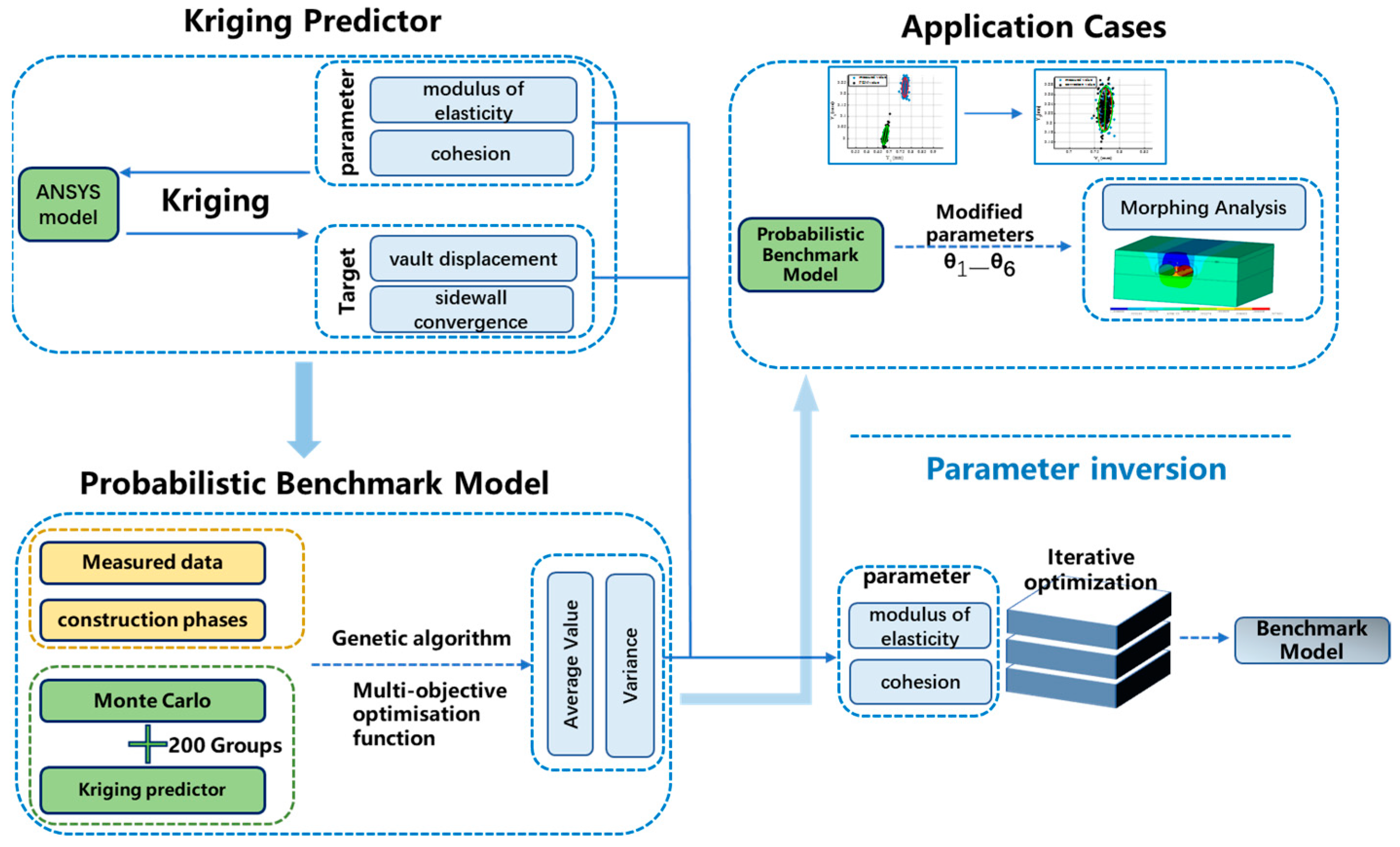
2.5. Methodological Procedures

Based on the above details, the inversion method for the surrounding rock parameters of the tunnel in a constructional environment of the probabilistic baseline model is summarized in the technical process, as shown in Figure 1.

3. Example of a Practical Tunnel

3.1. Yuhan Road Tunnel

The Yuhan Road Tunnel is an important part of the Jinan City Expressway Network Planning System tunnel support system in accordance with the principles of the new Austrian design, lining with composite lining, the initial support with anchors, reinforcing steel mesh, shotcrete, etc. to control the settlement of the tunnel, as well as the gradual stress relief process, the secondary lining with a thickness of 55 cm, the standard for C40-reinforced concrete.

This study focuses on the small clearance section of the tunnel in the Yuhan Road construction phase. The tunnel has the following dimensions: the radius of a side section of the tunnel is 6 m; the radius of the side wall is 11 m; the radius of the elevation arch is 15 m; and the top arch and side wall use an arc with a 3.7 m radius for the transition connection. The elevation arch and side wall use an arc with a 1.5 m radius for the transition connection, and the net width of the inner contour is 9.19 m. The net height of the tunnel is 7.3 m. The tunnel construction section schematic diagram is shown in Figure 2 and Figure 3.

The simulation of continuous tunnel construction in this study adopts the “applying virtual support force and gradually releasing method”. This method does not involve the superposition of the stress field and displacement field. The obtained displacement field and stress field from the solution represent the actual stress field and displacement field after tunnel excavation is completed. This approach is considered more reasonable for simulating the actual construction of tunnels [50].

To simulate the excavation of tunnel construction, ANSYS software is used. The support material parameters are set according to C25 reinforced concrete, considering the role of the steel arch. The diaphragm wall is made of C50 reinforced concrete. The physical and mechanical parameters are modified to simulate the reinforcing effect of the small conduit and the anchor rod [51]. These parameters are used as updating parameters in the numerical simulation. The material parameters for the simulation are presented in

Table 1. Tunnel material parameter values for small clearance sections.

Materials	Density (kg/m3)	Poisson’s Ratio	Young’s Modulus (MPa)	Cohesive Force (kPa)	Internal Friction Angle (°)
clay	1900	0.36	${\theta }_1$ = 36.8	${\theta }_4$ = 15	28
medium-weathering limestone	2000	0.35	${\theta }_2$ = 700	${\theta }_5$ = 160	25
medium-weathering marl	2100	0.35	${\theta }_3$ = 1100	${\theta }_6$ = 310	27
Anchor reinforcement zone	2040	0.32	910	208	30
Initial support for left and right guide holes	2400	0.2	36,200	/	/
look up in the air and vault	2400	0.2	33,000	/	/

. These parameters are adjusted to account for the reinforcing effect of the small conduit and the anchor rod, which ${\theta }_1\sim {\theta }_6$ is used as an updating parameter.

To eliminate the influence of boundary conditions and reduce calculation costs, the calculation area is taken to be approximately 4 times the diameter of the hole, based on the boundary effect model [50]. In this case, the model width is set to 80 m, with the bottom boundary of the tunnel extending 20 m down, the distance between the tunnel and the vertical boundary of the model is 16 m, and the longitudinal construction depth along the tunnel course is 70 m. The finite element model is established using different elements to represent different components. The solid45 solid unit is used to simulate the perimeter rock, anchor reinforcement area and part of the diaphragm wall. The shell63 shell unit is used to simulate the tunnel support structure. The mesh200 unit is used to mesh the plane cell and stretch it into a three-dimensional model. For the tunnel support structure, the shell63 unit is used, while the mesh200 unit is used to mesh the plane cell and stretch it into a three-dimensional model. The established finite element model of the tunnel with a small clear distance section consists of 157,811 nodes and 130,366 cells. In this model, the Y direction represents the vertical direction of the tunnel, the X direction represents the direction of the left and right boundaries of the tunnel, and the Z direction represents the longitudinal direction of the tunnel. Figure 4 shows the established finite element model of the tunnel.

3.2. Generation of the Tunnel Kriging Model

The physical and mechanical parameters of the surrounding rock are closely related to the vault displacement, and the most significant parameters for the physical mechanics of the surrounding rock are the Young’s modulus and the cohesive force. Therefore, the Young’s modulus and the cohesive force of the surrounding rock of the tunnel are adopted as the updating parameters, and the convergence value of the tunnel excavation side wall and the vault displacement are taken as the targets of the revision. On this basis, there are six updating parameters ${\theta }_1\sim {\theta }_6$ because the surrounding rock consists of three layers from top to bottom. In order to eliminate the boundary effect of the model, the settlement of the vault top after the completion of construction is corrected at the 10m, 30m and 60m positions of the progress in tunnel construction. The upper and lower limits of the updating parameters are 30%, and the average values of the updating parameters are shown in

Table 2. Initial Values of the Update Parameters (Units: Pa).

Parameter	E1	E2	E3	C1	C2	C3
Values	${\theta }_1\times 4\times {10}^7$	${\theta }_2\times 7\times {10}^8$	${\theta }_3\times 1.1\times {10}^9$	${\theta }_4\times 1.5\times {10}^4$	${\theta }_5\times 1.6\times {10}^5$	${\theta }_6\times 3.1\times {10}^5$

.

In order to address the computational redundancy problem of multi-objective optimization, based on the theoretical method of Kriging model construction in Section 4, the central composite design method is used to calculate the 44 groups of revised parameter sets [39], which is derived from the inversion parameter set of the tunnel model. The convergence of tunnel vault displacement and sidewall data are used to build a meta model using the above input (Young’s modulus and cohesion) and output (vault displacement and sidewall convergence) relationships.

To validate the accuracy of the constructed Kriging model, we extract the arch settlement and boundary wall convergence values of FEM at distances of 10 m, 30 m, and 60 m from the tunnel entrance as reference values and compared them with the deformation data of the constructed Kriging model. As shown in Figure 5, Figure 6, Figure 7, Figure 8, Figure 9 and Figure 10, it is found that the maximum value of the relative error of the constructed Kriging model is not more than 0.5%, so it is reasonable to establish the probability baseline model of tunnel with the generated Kriging model.

3.3. Generation of the Probabilistic Baseline of Tunnel FEM

In the stabilization phase after the completion of tunnel construction, the measured data have a certain fluctuation due to the testing error of instruments and human measurement, but the mean value is stabilized at a certain value. According to the theory in Section 2.3, the error between the statistical characteristics of the measured data and the results of FEM are defined as the objective function. Therefore, we first conduct statistical analysis on the monitoring data.

In the small, clear distance section of the tunnel, the left and right guide holes belong to a symmetrical structure. Due to the limitation of length, only one side is analyzed, and the actual monitoring data are represented in Figure 11, Figure 12, Figure 13, Figure 14, Figure 15 and Figure 16. In these figures, Y₁, Y₂ and Y₃ represent the converged displacement values of the side wall at distances of 10 m, 20 m and 30 m, respectively. Y₄, Y₅ and Y₆ represent the displacement values of the left tunnel arch at distances of 10 m, 20 m and 30 m, respectively.

From Figure 11, Figure 12, Figure 13, Figure 14, Figure 15 and Figure 16, it can be observed that the convergence value of the side wall under tunnel construction conditions tends to stabilize after 20 days, The red line in figure (b) confirms that the monitoring data of the stabilization phase correspond to the normal distribution. On the other hand, the settlement of the vault has already stabilized after 10 days. This implies that if only a certain cumulative value of the actual monitoring data is used as the updating target, the inverted parameters may not be applicable for the entire constructional environment. In other words, using a single cumulative value may not accurately capture the behavior and performance of the tunnel during the entire course of construction. It is necessary to consider the time-dependent behavior and variations in different sections of the tunnel during the construction process. Therefore, it is important to use a comprehensive approach that considers the entire constructional environment and takes into account the time-dependent behavior of the tunnel. This ensures that the inverted parameters are applicable and accurate for the entire construction process, rather than just a specific cumulative value.

In this section, a probabilistic baseline model updating algorithm based on the Kriging model was utilized to invert the parameters of the Yuhan Road tunnel. A multivariate normal distribution is assumed for the estimated values of the six parameters to be updated. To generate samples that satisfy the normal distribution, we employ a Monte Carlo simulation and generate 200 samples, some of the examples are listed in Appendix B. These samples are then statistically analyzed to calculate the means and covariances of the updated parameters. Furthermore, through the Kriging model, we calculate the values of sidewall convergence and arch settlement during tunnel construction. Statistical analysis is again performed to calculate the mean and covariance of these values. Using the construction measurement data gathered during tunnel construction, we establish a multi-objective optimization objective function to correct the finite element model. The Y₁ stability section acts as the horizontal coordinate, while the Y₂ to Y₆ construction phases serve as the vertical coordinates. We then plot the comparison diagrams before and after updating, as shown in Figure 17, Figure 18, Figure 19, Figure 20 and Figure 21. In these figures, the red areas represent the actual monitoring values, while the green areas depict the parameter values before and after correction. For further reference, the parameter values before and after correction are detailed in

Table 3. Comparing target displacement values before and after correcting the average target displacement.

Construction Section	Measured Displacement (mm)	Before Amendment		After Amendment
		Displacement Value (mm)	Relative Error (%)	Displacement Value (mm)	Relative Error (%)
Y1	0.77	0.6832	11.39	0.7716	0.08
Y2	0.81	0.7162	11.58	0.8084	0.2
Y3	0.89	0.7775	12.64	0.8916	0.18
Y4	3.41	3.1731	6.95	3.4151	0.15
Y5	3.23	3.1057	6.63	3.2301	0.00
Y6	3.12	2.9231	6.31	3.1201	0.00
ρ	1.00	0.8854	11.46	0.9548	4.52

and

Table 4. Comparison of updating parameters before and after model updating.

Rrevised Parameter	Initial Value	Revised Value	Revised Parameter	Initial Value	Revised Value
${\theta }_1$	36.8 MPa	47.83 MPa	$\mathit{Cov}({\theta }_1,{\theta }_4$)	−3.99	−3.44
${\theta }_2$	700 MPa	645.26 MPa	$\mathit{Cov}({\theta }_1,{\theta }_5$)	−7.82	−9.19
${\theta }_3$	1100 MPa	850.73 MPa	$\mathit{Cov}({\theta }_1,{\theta }_6$)	−1.70	−2.05
${\theta }_4$	15 Kpa	14.66 KPa	$\mathit{Cov}({\theta }_2,{\theta }_3$)	−2.11	−1.92
${\theta }_5$	160 Kpa	113.23 KPa	$\mathit{Cov}({\theta }_2,{\theta }_4$)	−2.69	−3.00
${\theta }_6$	310 Kpa	325.54 KPa	$\mathit{Cov}({\theta }_2,{\theta }_5$)	−6.42	−6.59
$\mathit{Var}({\theta }_1$)	17.38	15.56	Cov$({\theta }_2,{\theta }_6$)	−5.55	−6.54
$\mathit{Var}({\theta }_2$)	11.98	11.10	$\mathit{Cov}({\theta }_3,{\theta }_4$)	1.72	2.74
$\mathit{Var}({\theta }_3$)	3.06	2.43	$\mathit{Cov}({\theta }_3,{\theta }_5$)	−0.05	−1.04
$\mathit{Var}({\theta }_4$)	5.28	7.29	$\mathit{Cov}({\theta }_3,{\theta }_6$)	−0.02	0.07
$\mathit{Var}({\theta }_5$)	14.76	20.89	$\mathit{Cov}({\theta }_4,{\theta }_5$)	−1.83	−3.09
$\mathit{Var}({\theta }_6$)	6.13	11.53	$\mathit{Cov}({\theta }_4,{\theta }_6$)	1.85	2.88
$\mathit{Cov}({\theta }_1,{\theta }_2$)	2.48	1.00	$\mathit{Cov}({\theta }_5,{\theta }_6$)	0.27	−0.35
$\mathit{Cov}({\theta }_1,{\theta }_3$)	−2.65	−1.56

. These tables provide a comprehensive overview of the adjustments made during the updating process.

From Figure 17, Figure 18, Figure 19, Figure 20 and Figure 21, it can be observed that the distance between the centers of the two ellipses representing the analyzed data and the measured data is significantly reduced before and after updating the tunnel rock parameters. This indicates that parameter updating is effective in improving the accuracy of the model. According to Table 3, the initial error value between the analytical data and the measured data is 11.46% (with ρ equal to 0.8854). However, after parameter updating based on the probabilistic baseline model, the error of the model is significantly reduced to 4.52% (with ρ equal to 0.9548). It is worth noting that there is almost no error between the modeled data and the actual monitoring data, even in the stage of Y₅ and Y₆. Therefore, the model constructed based on the parameter inversion of this method can serve as a baseline model for the in-depth study of tunnel structure. The reduction in error and the close agreement between the modeled data and actual monitoring data demonstrate the validity and reliability of the probabilistic baseline model updating approach. This allows for a more accurate analysis and study of the tunnel structure, enhancing the understanding of its behavior and performance.

The mean target displacement values before and after model updating are shown in Table 3, and $\rho$ is the cosine similarity. A comparison of the parameters before and after model updating is shown in Table 4.

3.4. Practical Applications of the Tunnel Inversion Model

The above descriptions explain the selection method, sensitivity analysis and construction of the objective optimization function for the inversion of tunnel structural parameters based on a probabilistic baseline model. It also introduces the use of Kriging in combination with Monte Carlo random sampling to establish a Kriging model for the tunnel. To further demonstrate the effectiveness of the method, an engineering example is provided. In this example, the updated parameters ${\theta }_1$~${\theta }_6$ are incorporated into the finite element model of the tunnel. This analysis makes it possible to study the deformation and stress patterns that occur in the tunnel’s structural elements under the tunnel’s construction environment. This verification process helps to assess the performance and applicability of the method, ensuring a more reliable and accurate understanding of the tunnel’s behavior during construction and its ability to withstand the imposed loads and constraints.

Based on Figure 22, which displays the results of tunnel excavation using updated parameters in the analytical finite element, several key observations can be made:

(1)

Maximum displacement in the Y direction: The highest displacement occurs in the arch position of both the left and right guide holes, reaching 4.9 mm. This displacement indicates a significant settlement or deformation in the arch area. Additionally, there is a noticeable bulging phenomenon at the bottom of the tunnel arch, with a maximum displacement of 2.7 mm.

(2)

Influence of left and right guide holes: As the construction of the small clearance tunnel progresses, the left and right holes have minimal influence on each other. Therefore, the displacement cloud for both guide holes appears to be symmetrical, indicating similar settlement patterns.

(3)

Maximum negative displacement in the X direction: The largest negative displacement in the X direction is observed in the upper right position of the right guide hole, with a horizontal displacement of 1.8 mm. This indicates that there is significant movement or settlement towards the right side of the tunnel.

(4)

Maximum positive displacement in the X direction: The largest positive displacement in the X direction is located in the upper left position of the left guide hole, reaching 1.9 mm. This suggests significant movement or settlement towards the left side of the tunnel.

These displacement patterns highlight the importance of monitoring the settlement and deformation of tunnels during excavation to ensure structural stability and safety.

To eliminate the influence of the boundary effect in tunnel finite element simulation, the vault top points of left and left holes at 10 m position of tunnel excavation in longitudinal direction are taken as characteristic points, and their vertical displacement change curves are drawn. The changing graph of the displacement of the tunnel vault is shown in Figure 23.

Based on the information provided, it appears that during the construction of the center guide hole, settlement is observed in the vault of both the left and right guide holes. By the 20th construction step, the settlement of the arch top at the characteristic point of the right guide hole reaches 1.2 mm, while the settlement of the left guide hole stabilizes at around 1 mm. After the completion of the center guide hole construction and the pouring of the diaphragm walls, the excavation of the right guide hole is carried out. During this excavation, the settlement of the arch top in the right guide hole rapidly occurs and stabilizes in approximately 10 construction steps from the characteristic point. It seems that the excavation of the right guide hole has a minimal impact on the settlement of the left guide hole. When the excavation of the left guide hole takes place, it accelerates the settlement rate of the left guide hole. The displacement of the left guide hole stabilizes at around 10 construction steps from the characteristic point, with the settlement of both the left and right guide holes at the characteristic point stabilizing at 3.8 mm. It is important to carefully monitor and control the settlement and displacement of guide holes during construction to ensure the stability and safety of the structure.

4. Conclusions

The sample estimates of the displacements measured during tunnel construction serve as random variables due to the uncertain nature of the updating parameter and the structural deformation results obtained from the monitoring data. The probabilistic baseline model is applied to invert the surrounding rock parameters, and its applicability is verified through Monte Carlo random sampling and measured data. The following conclusions are drawn:

(1)

The inversion of tunnel surrounding rock parameters is carried out by introducing the parameter updating method of the probabilistic baseline model. With the comparative analysis of the mean and variance of measured data under different constructional environments, the inversion of tunnel surrounding rock parameters obtained by the proposed method has high accuracy and efficiency.

(2)

The Kriging model, combined with Monte Carlo random sampling, is used as an alternative model of the analytical FEM, and the results of the actual example show that the Kriging model is capable of accurately inverting physical parameters of a tunnel’s surrounding rock.

(3)

The accuracy of the parameter inversion decreases with the reduction of the amounts of measured data. Therefore, it is important to collect enough measured samples in order to generate a probabilistic baseline model with high accuracy.

(4)

The purpose of this research is not to directly analyze the structural deformation behavior under tunnel construction but to build probabilistic baseline models for different constructional environments. These models can be further utilized in deformation control and prediction research in tunnel construction.

References

1. Yu, Y.; Zhang, B.; Yuan, H. An intelligent displacement back-analysis method for earth-rockfill dams. Comput. Geotech. 2007, 34, 423–434. [Google Scholar] [CrossRef]
2. Qi, C.; Fourie, A.; Zhao, X. Back-Analysis Method for Stope Displacements Using Gradient-Boosted Regression Tree and Firefly Algorithm. J. Comput. Civ. Eng. 2018, 32, 04018031. [Google Scholar] [CrossRef]
3. Zhou, Z.; Liu, Y.; Dai, H.Z. Fully distributed strain-based output feedback for enhanced sensitivity in damage diagnosis of structures. Measurement 2023, 208, 112448. [Google Scholar] [CrossRef]
4. Chang, X.; Wang, H.; Zhang, Y. Back analysis of rock mass parameters in tunnel engineering using machine learning techniques. Comput. Geotech. 2023, 163, 105738. [Google Scholar] [CrossRef]
5. An, J.-S.; Song, K.-I. Back analysis of an operating subsea tunnel considering the degradation of ground and concrete lining. Mar. Georesources Geotechnol. 2019, 37, 517–523. [Google Scholar] [CrossRef]
6. Wu, C.; Hong, Y.; Chen, Q.; Karekal, S. A modified optimization algorithm for back analysis of properties for coupled stress-seepage field problems. Tunn. Undergr. Space Technol. 2019, 94, 103040. [Google Scholar] [CrossRef]
7. Pour, A.E.; Afrazi, M. Experimental Study of the Effect of Length and Angle of Cross-Cracks on Tensile Strength of Rock-Like Material. Iran. J. Sci. Technol. Trans. Civ. Eng. 2022, 46, 4543–4556. [Google Scholar] [CrossRef]
8. Majedi, M.R.; Afrazi, M.; Fakhimi, A. A Micromechanical Model for Simulation of Rock Failure Under High Strain Rate Loading. Int. J. Civ. Eng. 2021, 19, 501–515. [Google Scholar] [CrossRef]
9. Mottershead, J.E.; Friswell, M.I. Model updating in structural dynamics: A survey. J. Sound Vib. 1993, 167, 347–375. [Google Scholar] [CrossRef]
10. Zhang, Y.; Su, G.; Liu, B.; Li, T. A novel displacement back analysis method considering the displacement loss for underground rock mass engineering. Tunn. Undergr. Space Technol. 2020, 95, 103141. [Google Scholar] [CrossRef]
11. Ghorbani, E.; Moosavi, M.; Hossaini, M.F.; Assary, M.; Golabchi, Y. Determination of initial stress state and rock mass deformation modulus at Lavarak HEPP by back analysis using ant colony optimization and multivariable regression analysis. Bull. Eng. Geol. Environ. 2021, 80, 429–442. [Google Scholar] [CrossRef]
12. Guo, Q.; Pei, L.; Zhou, Z.; Chen, J.; Yao, F. Response surface and genetic method of deformation back analysis for high core rockfill dams. Comput. Geotech. 2016, 74, 132–140. [Google Scholar] [CrossRef]
13. Kolivand, F.; Rahmannejad, R. Estimation of geotechnical parameters using Taguchi’s design of experiment (DOE) and back analysis methods based on field measurement data. Bull. Eng. Geol. Environ. 2018, 77, 1763–1779. [Google Scholar] [CrossRef]
14. Wang, P.T.; Yang, T.H.; Xu, T.; Yu, Q.L.; Liu, H.L. A model of anisotropic property of seepage and stress for jointed rock mass. J. Appl. Math. 2013, 2013, 420536. [Google Scholar] [CrossRef]
15. Cheng, L.; Tong, F.; Li, Y.; Yang, J.; Zheng, D. Comparative study of the dynamic back-analysis methods of concrete gravity dams based on multivariate machine learning models. J. Earthq. Eng. 2021, 25, 1–22. [Google Scholar] [CrossRef]
16. Kong, P.; Jiang, L.; Shu, J.; Sainoki, A.; Wang, Q. Effect of fracture heterogeneity on rock mass stability in a highly heterogeneous underground roadway. Rock Mech. Rock Eng. 2019, 52, 4547–4564. [Google Scholar] [CrossRef]
17. Liu, Y.; Gao, M. Detecting cracks in concrete structures with the baseline model of the visual characteristics of images. Comput. Aided Civ. Infrastruct. Eng. 2022, 37, 1891–1913. [Google Scholar] [CrossRef]
18. Han, U.C.; Choe, C.S.; Hong, K.U.; Han, H.I. Intelligent back analysis of geotechnical parameters for time-dependent rock mass surrounding mine openings using grey Verhulst model. J. Cent. S. Univ. 2021, 28, 3099–3116. [Google Scholar] [CrossRef]
19. Mitelman, A.; Yang, B. Coupling Geotechnical Numerical Analysis with Machine Learning for Observational Method Projects. Geosciences 2023, 13, 196. [Google Scholar] [CrossRef]
20. Ching, J.; Phoon, K.K.; Chen, Y.C. Reducing shear strength uncertainties in clays by multivariate correlations. Can. Geotech. 2010, 47, 16–33. [Google Scholar]
21. Kelly, R.; Huang, J. Bayesian updating for one-dimensional consolidation measurements. Can. Geotech. 2015, 52, 1318–1330. [Google Scholar]
22. Zheng, D.; Huang, J.; Li, D.Q.; Kelly, R.; Sloan, S.W. Embankment prediction using testing data and monitored behaviour: A Bayesian updating approach. Comput. Geotech. 2018, 93, 150–162. [Google Scholar]
23. Song, Z.; Yang, Z. Inversion Analysis Method for Tunnel and Underground Space Engineering: A Short Review. Appl. Sci. 2023, 13, 5454. [Google Scholar] [CrossRef]
24. Gao, W.; Lu, X.; Peng, Y.; Wu, L. A Deep Learning Approach Replacing the Finite Difference Method for In Situ Stress Prediction. IEEE Access. 2020, 8, 44063–44074. [Google Scholar]
25. Li, Z.; Gong, W.; Li, T.; Juang, C.H.; Chen, J.; Wang, L. Probabilistic back analysis for improved reliability of geotechnical predictions considering parameters uncertainty, model bias, and observation error. Tunn. Undergr. Space Technol. 2021, 115, 104051. [Google Scholar] [CrossRef]
26. Zheng, H.; Mooney, M.; Gutierrez, M. Updating model parameters and predictions in SEM tunnelling using a surrogate-based Bayesian approach. Géotechnique, 2023; 1751–7656, ahead of print. [Google Scholar] [CrossRef]
27. Sui, Y.; Cheng, X.H. Investigation of cracking mechanism of the first tunnel lining during double-arch tunnel construction. Undergr. Space 2024, 14, 1–17. [Google Scholar] [CrossRef]
28. Zhou, Z.; Ma, X.; Liu, Y. A method for monitoring the uneven settlement of shield tunnels considering the flattening effect using distributed strain data measured from BOTDA sensors. Struct. Health Monit. 2024; OnlineFirst. [Google Scholar] [CrossRef]
29. Bin, L.; Gong, Z. Full-waveform inversion method for tunnel seismic forward prospecting. Geophys. J. Int. 2023, 232, 2186–2204. [Google Scholar] [CrossRef]
30. Sun, J.L.; Wu, S.C. Inversion of Surrounding Rock Mechanical Parameters in a Soft Rock Tunnel Based on a Hybrid Model EO-LightGBM. Rock Mech. Rock Eng. 2023, 56, 6691–6707. [Google Scholar] [CrossRef]
31. Cui, J.; Wu, S.; Cheng, H.; Kui, G.; Zhang, H.; Hu, M.; He, P. Composite interpretability optimization ensemble learning inversion surrounding rock mechanical parameters and support optimization in soft rock tunnels. Comput. Geotech. 2024, 165, 105877. [Google Scholar] [CrossRef]
32. Liu, Y.; Li, H.; Wang, Y.; Men, Y.; Xu, Q. Damage detection of tunnel based on the high-density cross-sectional curvature obtained using strain data from BOTDA sensors. Mech. Syst. Signal Process. 2021, 158, 107728. [Google Scholar] [CrossRef]
33. Farias, M.M.D.; Junior, A.H.M.; Assis, A.P.D. Displacement control in tunnels excavated by the NATM: 3-D numerical simulations. Tunn. Undergr. Space Technol. 2004, 19, 283–293. [Google Scholar] [CrossRef]
34. Minardo, A.; Catalano, E.; Coscetta, A.; Zeni, G.; Zhang, L.; Di Maio, C.; Vassallo, R.; Coviello, R.; Macchia, G.; Picarelli, L.; et al. Distributed fiber optic sensors for the monitoring of a tunnel crossing a landslide. Remote Sens. 2018, 10, 1291. [Google Scholar] [CrossRef]
35. Exadaktylos, G.E. On the constraints and relations of elastic constants of transversely isotropic geomaterials. Int. J. Rock Mech. Min. Sci. 2001, 38, 941–956. [Google Scholar]
36. Li, Y.Y.; Wang, Q.; Chen, J.P.; Xu, L.M.; Song, S.Y. K-means algorithm based on particle swarm optimization for the identification of rock discontinuity sets. Rock Mech. Rock Eng. 2014, 48, 375–385. [Google Scholar] [CrossRef]
37. Miro, S.; König, M.; Hartmann, D.; Schanz, T. A probabilistic analysis of subsoil parameters uncertainty impacts on tunnel-induced ground movements with a back analysis study. Comput. Geotech. 2015, 68, 38–53. [Google Scholar] [CrossRef]
38. Liu, Y.; Li, Y.; Wang, D.; Zhang, S. Model Updating of Complex Structures Using the Combination of Component Mode Synthesis and Kriging Predictor. Sci. World J. 2014, 13, 476219. [Google Scholar] [CrossRef]
39. Liu, Y.; Zhang, S. Probabilistic Baseline of Finite Element Model of Bridges under Environmental Temperature Changes. Comput. Aided Civ. Infrastruct. Eng. 2017, 32, 581–598. [Google Scholar] [CrossRef]
40. Adeli, H.; Jiang, X. Intelligent Infrastructure—Neural Networks, Wavelets, and Chaos Theory for Intelligent Transportation Systems and Smart Structures; CRC Press: Boca Raton, FL, USA, 2009. [Google Scholar] [CrossRef]
41. Sun, H.; Betti, R. A hybrid optimization algorithm with Bayesian inference for probabilistic model updating. Comput. Aided Civ. Infrastruct. Eng. 2015, 30, 602–619. [Google Scholar] [CrossRef]
42. Zhou, C.; Xiao, N.-C.; Zuo, M.J.; Gao, W. An active kriging based learning method for hybrid reliability analysis. IEEE Trans. Reliab. 2021, 71, 1567–1576. [Google Scholar] [CrossRef]
43. Boscato, G.; Russo, S.; Ceravolo, R.; Fragonara, L.Z. Global sensitivity-based model updating for heritage structures. Comput. Aided Civ. Infrastruct. Eng. 2015, 30, 620–635. [Google Scholar] [CrossRef]
44. Bernal, D. Sensitivities of eigenvalues and eigenvectors from complex perturbations, in Topics in Modal. Analysis II 2002, 6, 589–593. [Google Scholar] [CrossRef]
45. Jeong, S.; Murayama, M.; Yamamoto, K. Efficient optimization design method using kriging model. J. Aircr. 2005, 42, 413–420. [Google Scholar] [CrossRef]
46. Simpson, T.W.; Mauery, T.M.; Korte, J.J.; Mistree, F. Kriging models for global approximation in simulation-based multidisciplinary design optimization. AIAA J. 2001, 39, 2233–2241. [Google Scholar] [CrossRef]
47. Adeli, H.; Cheng, N.-T. Integrated genetic algorithm for optimization of space structures. J. Aerosp. Eng. 1993, 6, 315–328. [Google Scholar] [CrossRef]
48. Ronald, C. Plane Answers to Complex Questions: The Theory of Linear Models (Springer Texts in Statistics); Springer: Berlin/Heidelberg, Germany, 2011. [Google Scholar]
49. Guo, P.P.; Liu, F.F. Predicting Response of Constructed Tunnel to Adjacent Excavation with Dewatering. Geofluids 2021, 2021, 5548817. [Google Scholar] [CrossRef]
50. He, N.; Zhang, X. Excavation and Construction Technology of Diversion Tunnel under Complex Geological Conditions. Appl. Sci. 2023, 13, 11538. [Google Scholar] [CrossRef]
51. Fang, Q.; Tai, Q.; Zhang, D.; Wong, L.N.Y. Ground surface settlements due to construction of closely-spaced twin tunnels with different geometric arrangements. Tunn. Undergr. Space Technol. 2016, 51, 144–151. [Google Scholar] [CrossRef]
Figure 1. Flowchart of the proposed method.
Geosciences 14 00107 g001
Figure 2. Practical overview map.
Geosciences 14 00107 g002
Figure 3. Schematic diagram and photos of the tunnel.
Geosciences 14 00107 g003
Figure 4. Numerical simulation diagram.
Geosciences 14 00107 g004
Figure 5. Relative error of the convergence values of the left and right guideway sidewalls at the 10 m position of the tunnel.
Geosciences 14 00107 g005
Figure 6. Relative error of the convergence values of the left and right guideway sidewalls at the 30 m position of the tunnel.
Geosciences 14 00107 g006
Figure 7. Relative error of the convergence values of the left and right guideway sidewalls at the 60 m position of the tunnel.
Geosciences 14 00107 g007
Figure 8. Relative error of the displacement of the left and right guideway vaults at the 10 m position of the tunnel.
Geosciences 14 00107 g008
Figure 9. Relative error of the displacement of the left and right guideway vaults at the 30 m position of the tunnel.
Geosciences 14 00107 g009
Figure 10. Relative error of the displacement of the left and right guideway vaults at the 60 m position of the tunnel.
Geosciences 14 00107 g010
Figure 11. Y1 construction measurement results.
Geosciences 14 00107 g011
Figure 12. Y2 construction measurement results.
Geosciences 14 00107 g012
Figure 13. Y3 construction measurement results.
Geosciences 14 00107 g013
Figure 14. Y4 construction measurement results.
Geosciences 14 00107 g014
Figure 15. Y5 construction measurement results.
Geosciences 14 00107 g015
Figure 16. Y6 construction measurement results.
Geosciences 14 00107 g016
Figure 17. Comparison before and after FEM updating of the Y2 stabilizing area.
Geosciences 14 00107 g017
Figure 18. Comparison before and after FEM updating of the Y3 stabilizing area.
Geosciences 14 00107 g018
Figure 19. Comparison before and after FEM updating of the Y4 stabilizing area.
Geosciences 14 00107 g019
Figure 20. Comparison before and after FEM updating of the Y5 stabilizing area.
Geosciences 14 00107 g020
Figure 21. Comparison before and after FEM updating of the Y6 stabilizing area.
Geosciences 14 00107 g021
Figure 22. Displacement map of the surrounding rock in the small clearance section of the tunnel: (a) Y-direction displacement cloud; (b) X-direction displacement cloud.
Geosciences 14 00107 g022
Figure 23. Variation of arch displacement in small clearance tunnels: (a) Variation of vault displacement of the left guide hole; (b) Variation of vault displacement of the right guide hole.
Geosciences 14 00107 g023