

Sustainable Retaining Wall Solution as a Mitigation Strategy on Steep Slopes in Soft Rock Mass

1
Faculty of Civil Engineering, Transportation Engineering and Architecture, University of Maribor, Smetanova 17, 2000 Maribor, Slovenia
2
Faculty of Civil Engineering, Architecture and Geodesy, University of Split, Matice Hrvatske 15, 21000 Split, Croatia
*
Author to whom correspondence should be addressed.
Geosciences 2024, 14(4), 90; https://doi.org/10.3390/geosciences14040090
Submission received: 31 January 2024
/
Revised: 15 March 2024
/
Accepted: 20 March 2024
/
Published: 22 March 2024
(This article belongs to the Section Geomechanics)
Abstract
:Steep slopes in soft rock are characterized by their susceptibility to instability (rockfall, rockslide) due to weathering and erosion of the slope surface. This article deals with the problem of adapting to the increasing height of the scree slope. The construction of a retaining wall in a scree slope in front of a slope of soft rock with a steep face, where a very rapid weathering and erosion process of weathered material takes place, and the simultaneous deposition of material in front of the steep slope is a common solution. Changes in the geometry of the slope and the front scree are taken into account, and at the same time, sufficient safety against rockfall must be ensured. The analysis is shown on a specific example of a steep flysch slope near Split, Dalmatia. The retaining wall solutions are compared in terms of function, cost and sustainability. The construction of a single colossal, reinforced concrete retaining wall shows that this solution is not feasible due to the high construction costs and CO2 emissions of the retaining wall. A model was therefore developed to determine the height of the retaining walls for different construction time intervals and distances from the original rock face. The critical failure modes were investigated for various retaining wall solutions with regard to the highest degree of utilization of the resistance, which also allows the cost-optimized solutions to be determined. By building two or more successive retaining walls at suitable intervals and at an appropriate distance from the original rock face, construction costs and CO2 emissions can be significantly reduced.
Keywords:
retaining wall; erosion; rockfall; steep slope; flysch; sustainable design; cost optimization1. Introduction
Steep slopes in soft rock are characterized by their susceptibility to instability (rockfall, rockslide) due to weathering and erosion of the slope surface. The deposited material forms a scree (talus) slope in front of the weathered rock face that is at an angle to the shear properties of the deposited material. Over time, the mass of deposited material becomes larger and larger, and its edge moves further and further away from the slope base. Often, however, the usability of this front area is required due to necessary infrastructure, buildings, or other reasons. If the front of the slope is removed, the weathering and erosion process is further accelerated, leading to unstable conditions on the slope. Therefore, if the weathered material is not removed, and the slope should not move too far away from the initial wall, a barrier in the form of a retaining wall must be constructed to limit the area in which the slope material is deposited.
This paper deals with the problem of placing a retaining wall in a scree field in front of a slope of soft rock with a steep face, on which a very rapid weathering process and removal of weathered material and at the same time deposition of material in the front of the steep slope take place. Changes in the geometry of the slope and the front scree have been taken into account, provided that sufficient safety against rockfalls is ensured at the same time.
The model for weathering—scree accumulation was made based on Fisher–Lehmann’s mathematical model of step slope erosion [1,2]. A simple analytical model for such a retaining wall is presented, which takes into account its location and the temporal course of the weathering influences and thus the height of the slope at the position of the retaining wall as a function of its location and time. The result of the analysis is the position and geometry of the retaining wall, which should be optimal from various aspects, such as cost, environmental, or other. Previous studies show the environmental [3] and cost [4] comparison as well as the life cycle [5] assessment of earth-retaining walls, but the present work deals specifically with the design of retaining walls for steep slopes caused by weathering and erosion of soft rock. Al-Subari et al. [6] presented a simplified method to assess the environmental impact of embodied energy (EE) and carbon dioxide (CO2) emissions associated with earth-retaining walls. The results were presented using a real case of a slope movement where four different types of ERWs were proposed to stabilize the slope. Although several studies on the optimal design of individual earth-retaining walls based on construction costs [7,8,9,10] or life cycle assessments [11,12,13] have already been successfully carried out, none of the research work to date has dealt with the optimal design of several retaining walls that are successively built on top of each other over different periods of time. The provision of such an optimal design leads to the verification of several additional stability failure mechanisms.
The main novelty of the proposed research is that the developed model is able to determine the height of the retaining wall at any location in front of a steep slope, taking into account the rate of rock weathering. In addition, the height of several retaining walls can be determined at selected time intervals. Since several failure mechanisms can occur, all retaining wall solutions have been verified by internal and global stability, which allows us to identify the critical failure mechanism for different retaining wall types.
The analysis is shown using a specific example of a steep flysch slope near Split, Dalmatia. Three retaining wall solutions, a reinforced concrete wall, a gabion gravity retaining wall and a geosynthetic reinforced soil wall, are compared under functional, cost and environmental aspects.
2. Problematics of Erosion of Vertically Excavated Slopes in Soft Rock Masses
The International Society for Rock Mechanics (ISRM) designates rock with a uniaxial compressive strength (UCS) in the range of 0.25 MPa to 25 MPa as “extremely weak” to “weak” [14]. The limits of this range are defined according to the strength values of materials used in construction practice and the values of materials investigated in soil mechanics. The term “hard soils—soft rocks” used in the literature indicates that soft rocks are treated as a marginal group of geotechnical materials whose properties are to be extrapolated from the known areas of soil mechanics and rock mechanics, although the practice has shown that soft rocks represent only the middle part of a unique geotechnical scale [15]. In the study of soft rock slopes, as a rule, the following options are analyzed: firstly, the stability of the slope, secondly, the possibility of rockfall, and thirdly, the consequences of the weathering and erosion process. The analyses are carried out step by step with the following steps:
- Determination of geological conditions and geomechanical parameters.
- Geodetic measurements and design geometry of the slope.
- Analysis models (rockslide, rockfall, prediction of weathering—erosion—scree slope formation).
- Measures—geometric placement of the barrier.
- Analysis of the barrier (e.g., retaining wall).
It is important to distinguish between rockslide and rockfall, i.e., to investigate both processes. Rockslide is checked computationally on planar or spatial stability models, depending on the width of the landslide. Rockfall, on the other hand, is analyzed using kinematic models, where it is treated as a break, fall and slide, roll and/or bounce on a steep slope. In addition to rockslides and rockfall, it is important to define the processes of weathering and erosion that occur simultaneously. Weathering is a process in which the physical properties of the rock are altered by the simultaneous action of various influences (freezing, thawing, hydration, rooting, etc.) and may also be simply referred to as decomposition. Erosion, on the other hand, is the removal of material that moves by gravity and is deposited at the base of the slope.
If the weathering process is slow, it is treated on a geological time scale; however, for many soft rocks, the weathering process is so fast that it can be considered on an engineering time scale, i.e., in decades. The relationship between weathering and erosion processes may be balanced, unbalanced in favor of weathering, or unbalanced in favor of erosion. Considering the material and climatic characteristics of Dalmatia (see case study [16]), it is assumed that the ratio between these processes varies between balanced and unbalanced in favor of weathering, so that erosion usually takes place on already weathered material.
Marl from Eocene flysch strata is a type of soft rock whose mechanical properties can be changed rapidly and significantly on an engineering time scale. When dealing with excavations in this type of material, especially if the slope is of permanent character, the biggest two concerns should be long-term stability and the changes of slope geometry by combined weathering–erosion action.
In a short time after excavation, in which the excavated cut in marl is exposed to the influence of atmospheric agents, the weathering process starts to affect material on the slope surface [17]. Repeated cycles of wetting–drying, heating–cooling and freezing–thawing deteriorate marl on the free face of the cut slope until it degrades to mechanically soil-like material. Weathered material is afterward eroded and deposited at the bottom of the slope, creating scree (or talus)-shaped layers. Figure 1 presents an example of a typical abandoned cut in Eocene flysch, where marl is the dominant type of rock. The photo is taken one decade after initial excavation.
Weathered material in talus is at its first stage of the weathering process, mechanically classified as gravel-like material (Figure 2), which means that it is deposited at angles that correspond to the angle of internal friction of gravel-like materials. At later stages of slope geometry development, with further weathering acting on the material in the talus and an additional load of newly formed talus layers, the material changes further to fine-graded material. Water infiltration into the flysch layers can lead to hydraulic fractures, the seepage forces generated by the water flow within the flysch layers can exert additional stresses on the slopes and the increased pore water pressures can weaken the cohesion and frictional resistance of the flysch layers, making them more susceptible to slope stability failure [18]. With the presence of water and additional load, the material gains some cohesive properties as well [16]. Significant changes in shear strength have been observed at different degrees of soil saturation when seismic forces are applied [19,20]. Dashti et al. [21] used an experimental centrifuge test to explain the main effects of various parameters on the understanding of liquefaction-induced settlement of buildings with shallow foundations.
To better understand the evolution of slopes, it is necessary to make long-term observations of cuts in this type of material. It is important to gain insight into the time frame in which the entire process takes place, from the initial time of formation of a steep or vertical slope to its final transformation (Figure 3), based on long-term observations [22]. This is influenced by the time course of material loss on the free side of the slope and the formation of the embankment at the front side, which is predicted from observations (measurements).
The observed data of the annual erosion of the cut can later be used to calibrate known mathematical models [23], such as Bakker–Le Heux [24] or Fisher–Lehmann [1,2] models of erosion of vertical cuts (Figure 3). These models can be used to perform predictive analyses for simple cut slope without any mitigation measures [22]. The geometrical and physical parameters listed in Table 1 are used for the analysis.
3. Modeling of Weathering Process of Soft Rock Mass—Scree Accumulation
Different cliff degradation models have been developed in the past [25], and one based on the oldest and simplest Fisher–Lehmann model (Figure 4) is used in this paper. The main assumptions of the Fisher–Lehmann model are [23]:
- -
- There exists an initial straight slope of uniform material with a slope β steep enough so that scree transport is not restricted.
- -
- The slope has horizontal ground at its base and at its crest.
- -
- There is no standing water at the base.
- -
- Weathering results in a uniform retreat of all parts of the exposed free surface in a given time by the moving of fine scree, which can theoretically be approximated by infinitesimal increments.
- -
- Larger falls on discontinuities are not considered.
- -
- The resulting scree simultaneously accumulates at the cliff foot as straight-line debris with constant angle α < β.
Figure 4.
Fisher–Lehmann mathematical model of steep slope erosion.

Given the above assumptions, the term for determining the convex core of an intact rock takes the form:
where:
Parameter cs is a constant required for exact derivation, which is basically a measure of the looseness of the scattered material; the volume of rock/volume of scree is (1 − cs)/cs. Intriguing data in the design are the time span until the realization of the final shape of the slope and the change of the geometry of the face of the slope, i.e., the final position of the top of the slope and the foot of the cut.
The scree foot increases with time and at the end can be determined using an expression [23]:
And the height of scree is:
where yult means the final position of the face of the slope. The change in the geometry of the slope surface with time y(t) can be described by the following functions:
The final position of the slope yult at the final time of erosion tult can be determined by including z = h in Equation (1), which thus takes the form:
Increase of width of scree with time is expressed as:
And the final width of scree is:
The volume of eroded material dVer(t) in a certain time increment is:
where z(t) is the height of the convex core of an intact rock and dy(t) is the depth of erosion. The volume of scree material dVs(t) in the same time increment is:
Volume of scree increased with time to its final value:
The height of scree zs(t) at position y = 0 in a certain time t is:
The height of scree zs(y,t) at a certain position y and in a certain time t is:
4. Modeling of Scree Accumulation behind Retaining Wall
Weathering of the rock causes erosion, and the scree (gravel-like material) is accumulated at the base of the slope. The rate of scree accumulation at the base of the slope can be estimated using terrestrial laser scanning (TLS) or other surveying techniques. The accumulation of the scree increases the height of the slope, see Figure 5a. To reduce the risk of rockfall and maximize the functional area near the base of the slope, the most common solution is to build a retaining wall. However, the construction of a retaining wall further increases the height of the slope behind the wall due to the excess material in front of the wall. Figure 5b shows the increase in slope height when a retaining wall is included. The construction of only one high retaining wall for a planned lifetime of 100 years is not appropriate, because the wall will be oversized and underutilized. Therefore, it is more economical to construct multiple retaining walls in sequence. To calculate the height of each retaining wall at different times, the geometric problem must be solved.
The length of the slope l and the height of the slope h are increased with time t, while inclination of the slope α is constant with time. First, the initial inclination of the slope and location of the slope are defined with α, Ht=0 and Lt=0. The initial volume of the scree Vt=0 is:
By including the base retaining wall located at a distance x from the edge of the initial location of the slope Lt=0, the height in the front of the retaining wall at time t = 0 is calculated as Hwb,t=0 (see Figure 5a):
The volume of the scree without a retaining wall ΔVt=i (see Figure 5a) increases with the time t and is calculated as:
where Ht=i are increments of height and Lt=i are increments of length. The number of time intervals in which the volume of accumulated scree is calculated is determined by i.
By including a single retaining wall located at a distance x from the edge of initial location of the slope Lt=0, the volume in the front of the retaining wall at different time t is calculated as (see Figure 5b):
Figure 5a presents the volume of the scree at initial time t = 0 and increases with the time increments ti, without the retaining wall. The volume of the scree with the retaining wall (Figure 5b) needs to be the same at initial time t = 0 and when increasing with the time increments ti.
The height of the accumulated scree is calculated as:
The total height of the retaining wall is calculated as:
By including more retaining walls located at a distance x from the edge of the initial location of the slope Lt=0, the volume in the front of the retaining walls at different times t is calculated as (see Figure 5c):
As the scree is accumulated behind the retaining wall, the height of the accumulated scree is calculated as:
Finally, the total height of each retaining wall is calculated as:
As aforementioned, the accumulation of the scree depends on the rate of the weathering of the rock. Therefore, the height ht and length lt of the slope increase with the time, see Equations (45) and (46):
where coefficients a, b and c represent the rate of accumulation of the scree. It should be noted that coefficients a, b and c are obtained by an approximation function on the dataset of predicted weathering of the rock. The increment of the slope height is then calculated:
5. Modeling of the Retaining Wall
The time-dependent accumulation of scree behind the retaining wall is expressed with Hw,t=I, and it is used as input for dimensioning of the retaining wall. The retaining wall must be verified in accordance with Eurocode standards [26]; therefore, the five main conditions were defined in the form of five geotechnical constraints:
- Condition 1: bearing capacity failure.
- Condition 2: position of resultant (eccentricity).
- Condition 3: sliding failure.
- Condition 4: wall overturning.
- Condition 5: global stability analysis.
Along with those five main constraints, several other geotechnical and structural constraints must be verified that depend on retaining wall type. Three types of retaining wall were considered for protection from rockfall and scree accumulation, which are reinforced concrete retaining wall, gabions and geosynthetic reinforced soil (see Figure 6). For a reinforced concrete retaining wall, sufficient area of the steel must be determined in order to sustain bending and shear forces that govern in the concrete section.
In the design of a gabion wall, the assessment encompasses critical factors such as overturning, translation, eccentricity and the bearing capacity of the foundation soil. Additionally, a meticulous verification process is undertaken to address the individual joints between blocks, emphasizing the importance of robust connections within the structure. The individual sections of the gabion are checked for the maximum normal and shear stress.
In the design process of a geosynthetic reinforced soil or mechanically stabilized earth wall (MSE), a crucial step involves verifying the stability of a conceptual entity known as the fictitious structure [27,28]. This structure comprises the front face of the MSE wall and a curve that bounds the end points of the geo-reinforcements. The fictitious structure is subjected to calculated forces, reflecting the real-world conditions and pressures the MSE wall may experience. Similar to the verification process for a gravity retaining wall, engineers assess the fictitious structure for potential issues related to overturning and slip. Overturning analysis ensures that the wall remains stable under the influence of external loads, while slip analysis evaluates the potential for horizontal movement along the reinforcement elements. The forces in the checkerboard cross-section are determined from the calculated forces acting on a structure. This means that only the forces above the control cross-section are taken into account. Reinforcements introduce stabilizing forces that correspond to the lower value of the two load-bearing capacities, i.e., tear-off and pull-out. The most critical cross-section is also determined. The sliding of a reinforced soil block along a geo-reinforcement is also verified. To check this limit state, the critical slip surface is determined from the end of the given reinforcement. The shear forces (due to active pressures) and the resistance forces (friction between reinforcement and sliding block) are calculated and checked to see whether the resistance forces are greater than the activated shear forces. The reinforced block is bounded by the face of the wall, the verified geo-reinforcement, a vertical line passing through the end point of the geo-reinforcement and the terrain. The block is loaded by an active earth pressure and by stabilizing forces due to geo-reinforcements that exceed the boundary of the reinforced block, as well as by other forces. Finally, the global stability is verified [29]. Figure 6 shows the retaining wall subjected to earth pressure as a result of the scree accumulation. It should be noted that each retaining wall at selected time t is analyzed separately. The effects and resistances of the individual failure mechanisms and retaining wall types are calculated in the following section for a specific example of a steep flysch slope.
6. Application of the Developed Model of Scree Accumulation in a Case Study
A specific example of a steep flysch slope near Split, Croatia, was chosen for the case study. Eocene flysch is a type of soft rock whose mechanical properties can be changed rapidly and significantly on an engineering time scale (see Section 2).
Based on the results obtained during the exploration work, the value of the geological strength index (GSI) was determined according to the part of the geomechanical classification system RMR [30,31]. The rock strength and deformation modulus decrease with increasing faulting of the rock mass and are estimated here on the basis of the geological strength index (GSI) introduced by Hoek [32]. The generalized Hoek–Brown failure criterion [33,34] was applied using the computer program RocLab [35]. The GSI classification was used to determine the geomechanical parameters of the rock mass. All required rock mass parameters were either measured in the field, tested in the laboratory, calculated, or set as design values. Weathered material in scree (debris) is mechanically classified as gravel-like material with a friction angle of 36°.
6.1. Rockfall Modeling and Analysis
To design barriers and test their effectiveness, a statistical analysis program RocFall was used [35]. The rockfall model includes slope geometry, slope materials, seeder properties, simulation parameters and barrier and collector properties. A retaining wall is also a barrier on the surface of the slope to change the path of the rocks on their way down the slope. The properties of the barrier can be defined between completely inelastic and completely elastic (intermediate coefficients between 0 and 1).
For different geometries (depending on time) and for different positions of the barrier, the following results were calculated for rocks that strike the barrier (see Figure 7):
- Bounce height, needs to be smaller than height of barrier over slope surface.
- Total kinetic energy.
- Translational kinetic energy.
- Rotational kinetic energy.
- Translational velocity.
- Rotational velocity.
- Impact locations on the barrier.
The retaining wall also has the function of a barrier, so it must be designed to withstand the effects listed above. From results, it is evident that the height of the barrier shall at all times be at least 2 m higher than the level of the scree slope at the place of the barrier.
6.2. Erosion Model and Analysis
The Fisher–Lehmann model was confirmed to be the most suitable [22]. The same model can be used as the basis for models which include some form of retaining constructions (which is in focus of this paper), or other interventions made in the talus part of the slope, such as removal or compaction of talus material (Figure 8).
The initial inclination of the slope is defined with α = 36°, and location of the slope is defined with Lt=0 = 18.9 m. The height of the initial slope is calculated by Equation (50):
The increment of scree with the time t is predicted, and the dataset for this case study is given in Table 2. The best prediction was obtained by executing multiple regression using MS Excel software (Version 2301) with Data Analysis Add-in. The following nonlinear relationship was obtained:
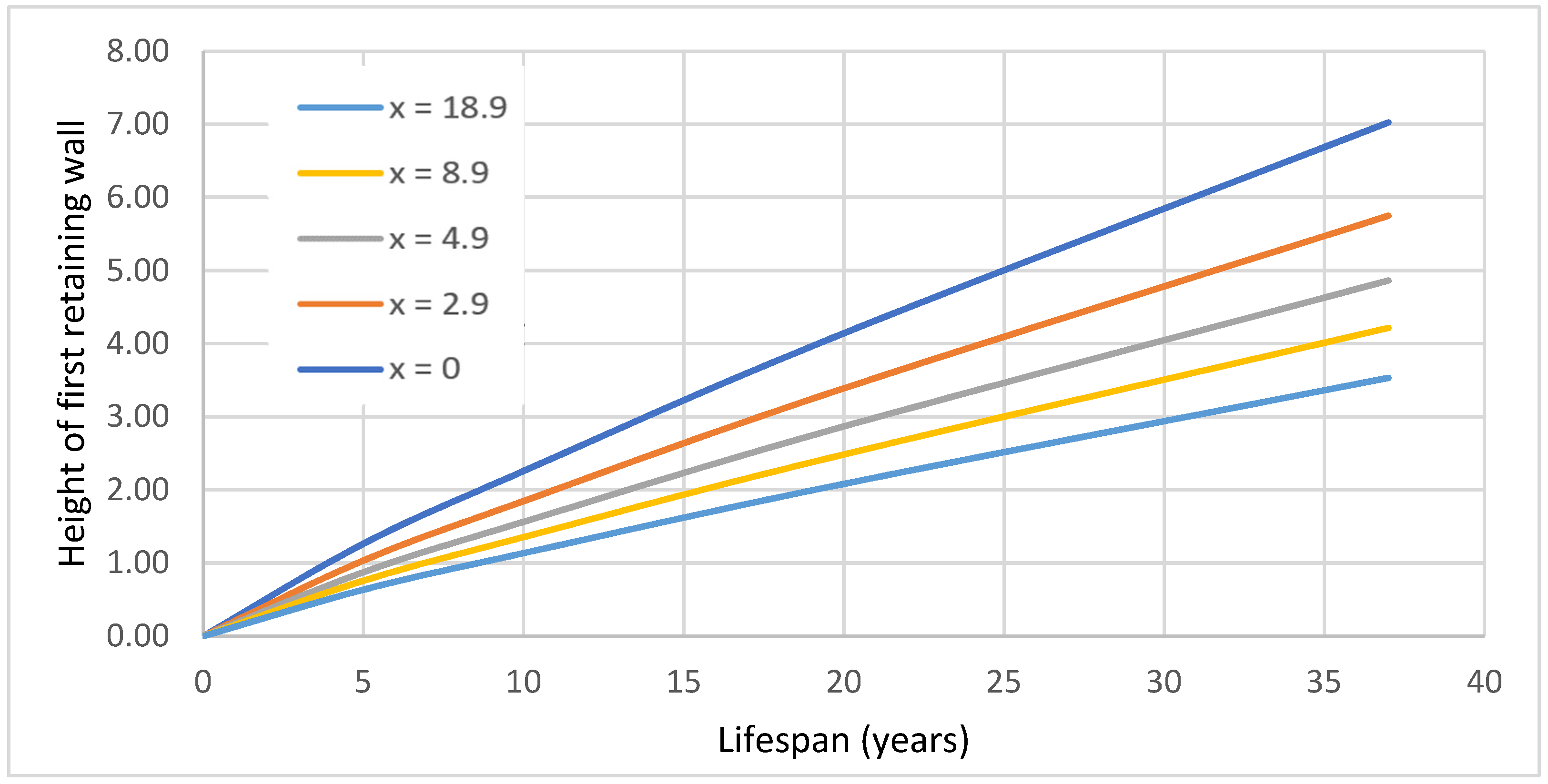
For predicted accumulation of the scree and by using Equation (34), the total height of the single retaining wall is calculated, and their values are presented in Figure 9. It should be noted that increasing the distance x also increases the height of the retaining wall Hw,t. By choosing the initial location of the retaining wall to be x = 0, the total height of the retaining wall should be 7.13 m (see Figure 9).
While the construction of only one high supporting wall for a planned lifetime of 100 years is not a good structural and economical solution, the second retaining wall after 37 years is planned to be constructed. In order to calculate the height of each retaining wall, Equations (34) and (44) are used. It should be noted that the distance ∆x was set to 1 m. Figure 10 summarizes the calculated results.
Therefore, the height of the first retaining (lower retaining wall) wall is Hw,t=37years = 3.53 m (see, Figure 10), and after the 37 years, the second retaining wall is constructed with a height of Hw,t=100years = 3.77 m (see, Figure 11). Figure 12 shows the required height of the retaining wall at various distances from the original rock slope.
Since the developed model enables us to determine the height of multiple retaining walls at a chosen time, in this case study, we also give the height of three retaining walls: the first retaining (lower retaining wall) wall is Hw,t=30years = 3.96 m, the second retaining (middle retaining wall) wall is Hw,t=60years = 2.31 m and the third retaining (upper retaining wall) wall is Hw,t=100years = 2.21 m.
6.3. Retaining Wall Model and Geotechnical Analysis
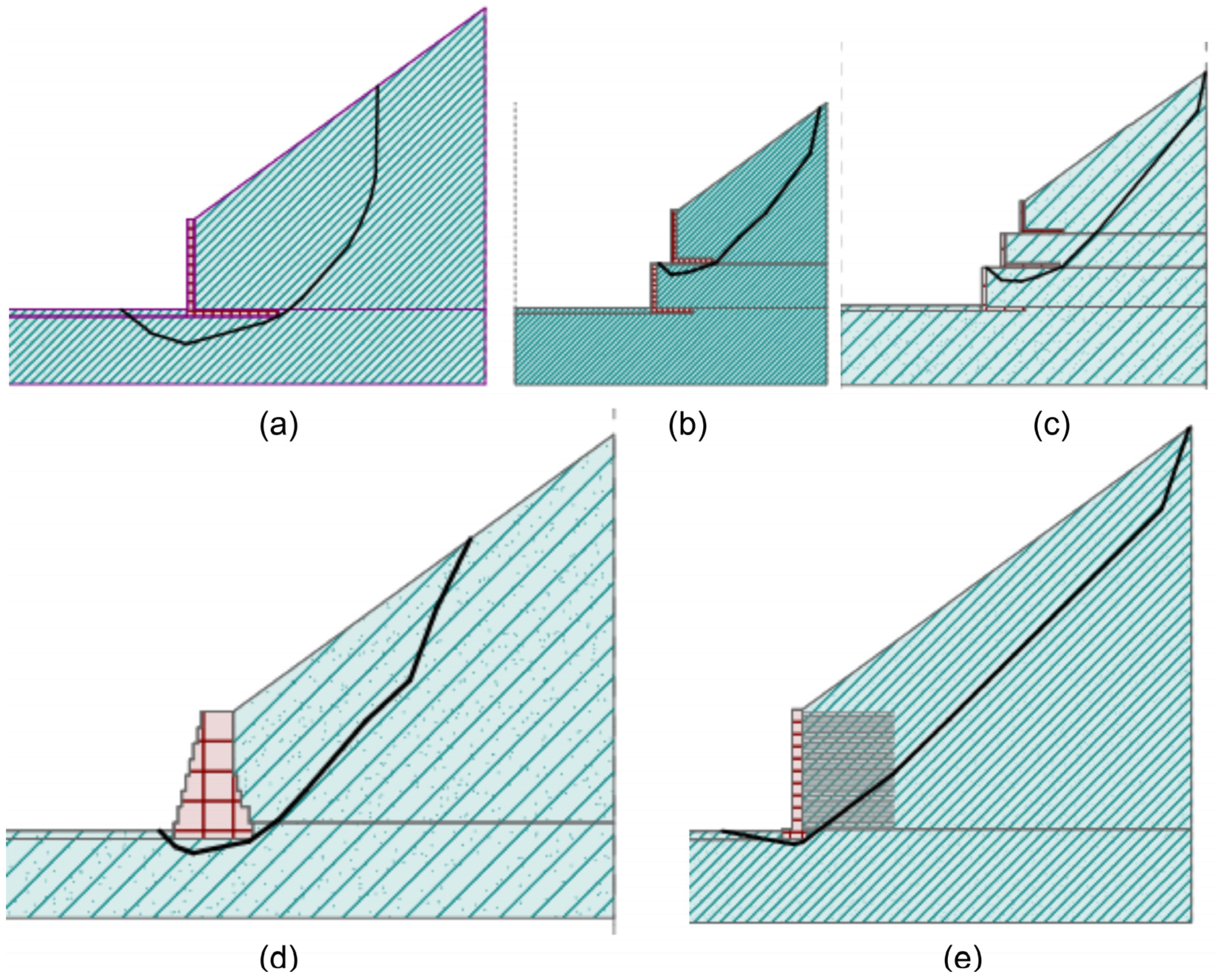
Three types of retaining walls were considered for protection from rockfall and scree accumulation, which are reinforced concrete retaining wall, gabions and geosynthetic reinforced soil. For the reinforced concrete retaining wall, three different options were analyzed, with one, two, or three retaining walls at different time intervals. For an L-shape reinforced concrete gravity wall, standard limit modes according to Eurocode standards were considered, including foundation failure, structural failure and overall stability. The design data comprise the unit weight of the scree γ (kN/m3), angle of internal friction φ (°), angle of friction soil-wall δ (°), the slope angle of retained material α (°) and the surcharge load p (kPa). The input data also include all the defined values of the dimensions and material properties of the retaining wall. All the input data for retaining wall verification are given in Table 3 and are shown in Figure 13. The most important design criterion for a single RC retaining wall is the load-bearing capacity of the foundation. For two and three RC retaining walls, ensuring global slope stability is the main criterion for achieving adequate support of retained soil. As soon as the slip lines between the upper and lower RC retaining walls are prevented, all other local stability requirements are also met. The critical failure lines for each type of retaining wall are shown in Figure 14. The gabions and MSE are also designed to achieve a high utilization rate for global slope stability. For the gabions, all individual joints between the blocks are checked for maximum normal and shear stress. The geosynthetic reinforcements have been designed to provide sufficient resistance to tearing and pull-out.
7. Cost and Environmental Comparisons of Retaining Walls
Table 4 provides a comprehensive overview of the main parameters for different types of retaining walls, focusing on structural, economic and environmental considerations. The table is organized into columns representing different types of retaining walls: single retaining wall, two retaining walls, three retaining walls, gabions and mechanically stabilized earth (MSE). The rows of the table include various parameters and their corresponding values for each retaining wall type. Structural parameters such as the weight of the structure (Ww), volume of the structure (Vw), mass of steel reinforcement (msteel), area of geosynthetic reinforcement (Ageo), volume of the foundation of the front batter (Vfound) and volume of the batter (Vbatter) are presented. All these geometric parameters are given per meter width of the retaining wall. The mass of the steel reinforcement is calculated on the basis of the determined ratio between the mass of the steel and the volume of the concrete, which is 130 kg/m3. Economic aspects are detailed through unit prices for concrete (ccon), steel (csteel), gabions (cgabions), geosynthetic reinforcement (cgeo), the front batter (cbatter) and reinforced fill soil (cfill). Environmental considerations are addressed by indicating unit emissions for concrete (cicon), reinforcement steel (cisteel), gabions (cigabions), geosynthetic reinforcement (cigeo), front batter (cibatter) and reinforced fill soil (cifill) in terms of kilograms of CO2. The material costs (COSTmat) are given for each type of retaining wall and the material costs associated with the amount of material used to build the wall each retaining wall are summarized. The total cost of construction of a retaining wall (COSTtotal) are also determined. In order to take into account the construction costs, which, together with the material costs, represent the total costs, the ratio between construction costs and material was considered for each type of retaining wall. The share of material costs and the share of labor costs were determined according to Eurostat instructions and the methodology of the Chambers of Commerce in Central Europe [36,37]. However, these percentages may vary depending on factors such as the complexity of the wall design, accessibility of the construction site and local labor costs. The following ratios were used for reinforced concrete walls, gabions and MSE, namely 1, 0.2 and 0.5, respectively.
This comprehensive table facilitates a detailed comparison of different retaining wall options, considering economic factors and environmental impact. The weight of the structure (Ww) is highest for the MSE wall, followed by gabions, single RC retaining wall, two RC retaining walls and three RC retaining walls. Solutions with two and three RC retaining walls and the MSE wall contribute a similar amount of CO2 emissions, with the highest emissions calculated for the single RC retaining wall, while the gabion wall had the lowest values. In terms of material and total costs, the MSE is determined to be the most economical solution.
8. Discussion and Conclusions
The problems of steep slopes in soft rock are discussed, which are characterized by a susceptibility to instability, which is reflected as weathering and erosion, rock slides and rockfalls. This work is limited to a slope of soft rock with a steep face, where a very rapid weathering process and erosion of weathered material takes place.
A model of weathering—scree accumulation was developed, which takes into account Fisher–Lehmann’s mathematical model of step slope erosion. The model makes it possible to calculate the height of the scree (debris) at any distance from the weathering stone slope and at any time. The problem is setting up a retaining wall on scree in front of a slope of soft rock with a steep wall, where a very rapid process of weathering and erosion removal of weathered material takes place and, at the same time, the material is deposited in front of the steep slope. Changes in the geometry of the slope and the front scree are taken into account, while, at the same time, ensuring sufficient safety against rockfall. A model of weathering—scree accumulation enables the calculation of the required height of the retaining wall, from one vertical segment or several.
A simple analytical model for a retaining wall is shown, which takes into account the position, time and inclination of the retaining wall. The result of the analysis is the position and geometry of the retaining wall, which should be optimal from various points of view, such as technical, functional, cost, or environmental aspects. Since the presented research work includes the determination of the optimal location of the retaining wall in front of the rock slope and the optimal design of the retaining wall, but these are achieved in two separate optimization processes, further research could integrate both design processes, which would lead to global optimal solutions. Extending the proposed model to include a life cycle analysis could contribute to a more sustainable wall design, as the current model assesses the environmental impact solely on the basis of CO2 emissions.
The applicability of the analysis is shown on a specific example of a steep flysch slope near Split, Dalmatia. Retaining wall solutions such as a reinforced concrete wall within one, two, or more height segments, a gabion gravity retaining wall and a wall made of geosynthetically reinforced soil are compared. All the walls are dimensioned to optimize costs.
A reinforced concrete retaining wall consisting of one segment is technically sufficient and complies with the European standards but is not functionally useful, as it has to be built immediately. Such a wall is also more expensive and less environmentally friendly. A reinforced concrete wall consisting of two or more segments allows adaptation to the erosion process over time. In terms of construction cost and environment (CO2 emissions), a wall consisting of two or more segments is acceptable compared to the other retaining wall types. The main critical failure mechanisms in a single retaining wall are bearing capacity and sliding failure, while global stability failure was identified as a critical failure mode when two or three segments of walls were used.
The gabion wall makes functional sense, as the installation of gabions allows a complete height adjustment of the scree slope and, at the same time, provides the best protection against rockfall. Such a wall is cost-effective compared to reinforced concrete but more expensive than a wall made of geosynthetically reinforced soil. The CO2 consumption is significantly lower than for the other compared retaining walls. This conclusion is in line with the results of Balasbaneh et al. [4], where the gabion retaining wall was also rated as the most environmentally friendly of all alternatives. In terms of construction costs, the reinforced concrete wall with three successive retaining walls is the best option, costing around 20% less than the gabion retaining wall. Here, too, Balasbaneh et al. [4] reported that the cantilever concrete wall costs around 17% less than the gabion wall.
The installation of geosynthetics enables complete adaptation to the height of the scree slope. Although this type of retaining wall is the cheapest, the CO2 emissions are higher than with a gabion wall. For the gabion and MSE retaining walls, global stability and sliding failure were the main conditions for the optimal design of the retaining wall. Damians et al. [38] assessed environmental impact of the several retaining wall structures including the MSE retaining wall and plotted results based on the wall heights. At the 7.2 m wall height presented in this case study, the natural resource endpoint indicator for MSE was about 60% lower than for concrete retaining walls [38], while in the case study presented, MSE caused about 47% less CO2 emissions. In this study, similar observations were made to those reported by Damians et al. [11] that MSEs are cheaper than other types of retaining walls at greater retaining wall heights. Koerner et al. [39] estimate that construction costs of 30–50% can be saved with MSE compared to traditional gravity retaining walls. In the case study presented in this article, the MSE was 32% cheaper than the reinforced concrete retaining wall. Further research into the economic and environmental benefits of different construction methods when building several retaining walls in succession in terms of reducing energy consumption and emissions of climate-relevant gases, as well as full life cycle assessments [40], are required to find a fully sustainable solution.
Author Contributions
Conceptualization, P.J., B.Ž. and G.V.; methodology, P.J., B.Ž. and G.V; software, P.J., B.Ž. and G.V.; validation, P.J., B.Ž. and G.V.; writing—original draft preparation, P.J., B.Ž. and G.V.; writing—review and editing, P.J., B.Ž. and G.V. All authors have read and agreed to the published version of the manuscript.
Funding
This research was funded by the Slovenian Research Agency (ARIS) and Ministry of Science and Education of Republic of Croatia by supporting a bilateral project (grant number BI-HR/23-24-023). This research was partly supported by the EU project GEOLAB (grant number 101006512) and a project co-financed by the Croatian Government and the European Union through the European Regional Development Fund—the Competitiveness and Cohesion Operational Programme (grant number KK.01.1.1.02.0027).
Data Availability Statement
The data presented in this study are available on request from the corresponding author.
Conflicts of Interest
The authors declare no conflict of interest.
References
- Fisher, O. On the Disintegration of a Chalk Cliff. Geol. Mag. 1866, 3, 354–356. [Google Scholar] [CrossRef]
- Lehman, O. Morphologische theorie der verwitterung von steinschlagwanden. Vierteljahrsschr. Naturforschenden Ges. Zur. 1933, 78, 83–126. [Google Scholar]
- Pons, J.J.; Penadés-Plà, V.; Yepes, V.; Martí, J.V. Life cycle assessment of earth-retaining walls: An environmental comparison. J. Clean. Prod. 2018, 192, 411–420. [Google Scholar] [CrossRef]
- Balasbaneh, A.T.; Yeoh, D.; Juki, M.I.; Ibrahim, M.H.W.; Abidin, A.R.Z. Assessing the life cycle study of alternative earth-retaining walls from an environmental and economic viewpoint. Environ. Sci. Pollut. Res. 2021, 28, 37387–37399. [Google Scholar] [CrossRef] [PubMed]
- Balasbaneh, A.T. Applying multi-criteria decision-making on alternatives for earth-retaining walls: LCA, LCC, and S-LCA. Int. J. Life Cycle Assess. 2020, 25, 2140–2153. [Google Scholar] [CrossRef]
- Al-Subari, L.; Yaqubi, N.A.; Selcukhan, O.; Ekinci, A. Environmental and economical assessment of earth-retaining walls for design optimisation. Environ. Geotech. 2022, 40, 1–18. [Google Scholar] [CrossRef]
- Kaveh, A.; Soleimani, N. CBO and DPSO for optimum design of reinforced concrete cantilever retaining walls. Asian J. Civ. Eng. 2015, 16, 751–774. [Google Scholar]
- Kaveh, A.; Kalateh-Ahani, M.; Fahimi-Farzam, M. Constructability optimal design of reinforced concrete retaining walls using a multi-objective genetic algorithm. Struct. Eng. Mech. 2013, 47, 227–245. [Google Scholar] [CrossRef]
- Basha, B.M.; Babu, G.L.S. Reliability Based Design Optimization of Gravity Retaining Walls. In Proceedings of the Probabilistic Applications in Geotechnical Engineering; American Society of Civil Engineers: Reston, VA, USA, 2007; pp. 1–10. [Google Scholar]
- Sadoglu, E. Design optimization for symmetrical gravity retaining walls. Acta Geotech. Slov. 2014, 11, 71–79. [Google Scholar]
- Damians, I.P.; Bathurst, R.J.; Adroguer, E.G.; Josa, A.; Lloret, A. Sustainability assessment of earth-retaining wall structures. Environ. Geotech. 2018, 5, 187–203. [Google Scholar] [CrossRef]
- Zastrow, P.; Molina-Moreno, F.; García-Segura, T.; Martí, J.V.; Yepes, V. Life cycle assessment of cost-optimized buttress earth-retaining walls: A parametric study. J. Clean. Prod. 2017, 140, 1037–1048. [Google Scholar] [CrossRef]
- Feng, G.; Luo, Q.; Lyu, P.; Connolly, D.P.; Wang, T. An Analysis of Dynamics of Retaining Wall Supported Embankments: Towards More Sustainable Railway Designs. Sustainability 2023, 15, 7984. [Google Scholar] [CrossRef]
- Ulusay, R. (Ed.) The ISRM Suggested Methods for Rock Characterization, Testing and Monitoring: 2007–2014; Springer International Publishing: Cham, Switzerland, 2015; ISBN 978-3-319-07712-3. [Google Scholar]
- Evangelista, A. International Symposium on Hard Soils-Soft Rocks. In The Geotechnics of Hard Soils-Soft Rocks: Proceedings of the Second International Symposium on Hard Soils-Soft Rocks, Naples, Italy, 12–14 October 1998; Evangelista, A., Ed.; Balkema: Rotterdam, The Netherlands, 1998; Volume 1. [Google Scholar]
- Vlastelica, G.; Mišcevic, P.; Štambuk Cvitanovic, N.; Glibota, A. Geomechanical aspects of remediation of quarries in the flysch: Case study of abandoned quarry in Majdan, Croatia. In Proceedings of the ISRM EUROCK, Saint Petersburg, Russia, 22–26 May 2018. [Google Scholar]
- Miščević, P.; Vlastelica, G. Impact of weathering on slope stability in soft rock mass. J. Rock Mech. Geotech. Eng. 2014, 6, 240–250. [Google Scholar] [CrossRef]
- Fell, R.; Corominas, J.; Bonnard, C.; Cascini, L.; Leroi, E.; Savage, W.Z. Guidelines for landslide susceptibility, hazard and risk zoning for land-use planning. Eng. Geol. 2008, 102, 99–111. [Google Scholar] [CrossRef]
- Forcellini, D. The Role of the Water Level in the Assessment of Seismic Vulnerability for the 23 November 1980 Irpinia–Basilicata Earthquake. Geosciences 2020, 10, 229. [Google Scholar] [CrossRef]
- Forcellini, D. Seismic assessment of a benchmark based isolated ordinary building with soil structure interaction. Bull. Earthq. Eng. 2018, 16, 2021–2042. [Google Scholar] [CrossRef]
- Dashti, S.; Bray, J.D.; Pestana, J.M.; Riemer, M.; Wilson, D. Mechanisms of Seismically Induced Settlement of Buildings with Shallow Foundations on Liquefiable Soil. J. Geotech. Geoenviron. Eng. 2010, 136, 151–164. [Google Scholar] [CrossRef]
- Vlastelica, G.; Miscevic, P.; Fukuoka, H. Monitoring of vertical cuts in soft rock mass, defining erosion rates and modelling time-dependent geometrical development of the slope. In Proceedings of the ISRM EUROCK, Ürgüp, Turkey, 29–31 August 2016. [Google Scholar]
- Hutchinson, J.N. A small-scale field check on the Fisher–Lehmann and Bakker–Le Heux cliff degradation models. Earth Surf. Process. Landf. J. Br. Geomorphol. Gr. 1998, 23, 913–926. [Google Scholar] [CrossRef]
- Bakker, J.P.; Le Heux, J.W.N. Projective-Geometric Treatment of O. Lehmann’s Theory of the Transformation of Steep Mountain Slopes; North-Holland Publishing Company: Amsterdam, The Netherlands, 1946. [Google Scholar]
- Carson, M.A.; Kirkby, M.J. Hillslope Form and Process; Cambridge University Press: Cambridge, UK, 1972. [Google Scholar]
- EN 1997-1; Eurocode 7: Geotechnical Design—Part 1: General Rules. BSI: London, UK, 2004; ISBN 9780580671067/0580671062/0580452123/9780580452123.
- Jelušič, P.; Žlender, B. Determining optimal designs for geosynthetic-reinforced soil bridge abutments. Soft Comput. 2020, 24, 3601–3614. [Google Scholar] [CrossRef]
- Recommendations for Design and Analysis of Earth Structures Using Geosynthetic Reinforcements–EBGEO; Wiley: Hoboken, NJ, USA, 2012; ISBN 9783433029831.
- Jelušič, P.; Žlender, B.; Dolinar, B. NLP Optimization Model as a Failure Mechanism for Geosynthetic Reinforced Slopes Subjected to Pore-Water Pressure. Int. J. Geomech. 2016, 16, C4015003. [Google Scholar] [CrossRef]
- Bieniawski, Z.T. Engineering Rock Mass Classifications: A Complete Manual for Engineers and Geologists in Mining, Civil, and Petroleum Engineering; John Wiley & Sons: Hoboken, NJ, USA, 1989; ISBN 0471601721. [Google Scholar]
- Bieniawski, Z.T. Engineering classification of jointed rock masses. Civ. Eng. S. Afr. 1974, 11, 98. [Google Scholar] [CrossRef]
- Hoek, E.; Brown, E.T. Practical estimates of rock mass strength. Int. J. Rock Mech. Min. Sci. 1997, 34, 1165–1186. [Google Scholar] [CrossRef]
- Hoek, E.; Carranza-Torres, C.; Corkum, B. Hoek-Brown failure criterion-2002 edition. In Proceedings of the NARMS-TAC Conference, Toronto, ON, Canada, 7–10 July 2002; Volume 1, pp. 267–273. [Google Scholar]
- Hoek, E.; Diederichs, M.S. Empirical estimation of rock mass modulus. Int. J. Rock Mech. Min. Sci. 2006, 43, 203–215. [Google Scholar] [CrossRef]
- RocFall3 User Guide Documentation and Theory Overview. Available online: https://www.rocscience.com/help/rocfall3/overview (accessed on 10 February 2024).
- Pšunder, M.; Klanšek, U.; Šuman, N. Gradbeno Poslovanje; 1. ponatis; Fakulteta za Gradbeništvo: Maribor, Slovenia, 2012; ISBN 9789612481599/9612481598. [Google Scholar]
- Žemva, S. Gradbene Kalkulacije in Obračun Gradbenih Objektov: Priročnik za Prakso; 3. dopolnj; Gospodarska zbornica Slovenije, Center za poslovno usposabljanje: Ljubljana, Slovenia, 2023; ISBN 978-961-6924-02-3. [Google Scholar]
- Damians, I.P.; Bathurst, R.J.; Adroguer, E.G.; Josa, A.; Lloret, A. Environmental assessment of earth retaining wall structures. Environ. Geotech. 2017, 4, 415–431. [Google Scholar] [CrossRef]
- Koerner, R.; Koerner, J.; Soong, T.-Y. Earth Retaining Wall Costs in the USA; Geosynthetic Research Institute: Folsom, PA, USA, 2001; pp. 483–506. [Google Scholar]
- Heerten, G. Reduction of climate-damaging gases in geotechnical engineering practice using geosynthetics. Geotext. Geomembr. 2012, 30, 43–49. [Google Scholar] [CrossRef]
Figure 1.
Example of typical abandoned cut in Eocene flysch.

Figure 2.
Example of marl deterioration by process of wetting and drying (WD): (a) intact material taken immediately after excavation; (b) same material after one WD cycle; (c) same material after two WD cycles; (d) same material after four WD cycles.
Figure 2.
Example of marl deterioration by process of wetting and drying (WD): (a) intact material taken immediately after excavation; (b) same material after one WD cycle; (c) same material after two WD cycles; (d) same material after four WD cycles.

Figure 3.
Formation of a steep slope from the initial time to its final transformation.

Figure 5.
Accumulation of the scree (a) without retaining wall (b) with single retaining wall (c) with multiple offset retaining walls.
Figure 5.
Accumulation of the scree (a) without retaining wall (b) with single retaining wall (c) with multiple offset retaining walls.

Figure 6.
Different types of the protective retaining walls: (a) reinforced concrete retaining wall, (b) gabion wall and (c) geosynthetic reinforced soil.
Figure 6.
Different types of the protective retaining walls: (a) reinforced concrete retaining wall, (b) gabion wall and (c) geosynthetic reinforced soil.

Figure 7.
Rockfall modeling. (a) Slope geometry and (b) rock block trajectories without barrier, t = 0 [16].
Figure 7.
Rockfall modeling. (a) Slope geometry and (b) rock block trajectories without barrier, t = 0 [16].

Figure 8.
Prediction of scree accumulation.

Figure 9.
The total height of the single retaining wall for a given lifespan.

Figure 10.
The total height of the first (bottom) retaining wall for a given lifespan.

Figure 11.
The total height of the second (upper) retaining wall for a given lifespan.

Figure 12.
The total heights of retaining walls for a given lifespan.

Figure 13.
Retaining wall geometry: (a) single retaining wall, (b) upper retaining wall and (c) lower retaining wall.
Figure 13.
Retaining wall geometry: (a) single retaining wall, (b) upper retaining wall and (c) lower retaining wall.

Figure 14.
The critical failure lines for various types of retaining walls: (a) single retaining wall, (b) two retaining walls, (c) three retaining walls, (d) gabion wall and (e) geosynthetic reinforced slope.
Figure 14.
The critical failure lines for various types of retaining walls: (a) single retaining wall, (b) two retaining walls, (c) three retaining walls, (d) gabion wall and (e) geosynthetic reinforced slope.


Table 1.
Geometrical and physical parameters of slope.
| Geometrical Parameters | Symbol | Physical Parameters | Symbol |
|---|---|---|---|
| Width of scree | ys (m) | Density of initial rock | γr (kg/m3) |
| Inclination of scree slope | α (⁰) | Average year erosion | Ry,s (cm/year) |
| Deviation of the convex core | y (m) | Density of scree | γs (kg/m3) |
| Inclination of initial slope | β1 (⁰) | Scree volume increase coefficient | cs |
| Inclination of slope | β2 (⁰) | Cohesion of scree | c (kPa) |
| Height of slope | h (m) | Shear angle of scree | φ (⁰) |
| Position of retaining wall | yR (m) | ||
| Height of retaining wall | hR (m) |
Table 2.
Predicted accumulation of the scree increase as a function of time.
| t (Years) | 0 | 5 | 10 | 20 | 50 | 100 |
|---|---|---|---|---|---|---|
| lt (m) | 18.9 | 19.6 | 20.3 | 21.5 | 24.1 | 26.9 |
| ht (m) | 13.7 | 14.2 | 14.8 | 15.6 | 17.5 | 19.5 |
Table 3.
The verification of the retaining walls (initial location of the retaining wall x = 0).
| Single Retaining Wall (See Figure 5a) | Two Retaining Walls | Three Retaining Walls | Gabions | MSE | ||||
|---|---|---|---|---|---|---|---|---|
| Upper Wall (See Figure 5b) | Lower Wall (See Figure 5c) | Upper Wall | Middle Wall | Lower Wall | ||||
| Soil properties | ||||||||
| γ (kN/m3) | 19 | 19 | 19 | 19 | 19 | 19 | 19 | 19 |
| φ (°) | 36 | 36 | 36 | 36 | 36 | 36 | 36 | 36 |
| c (kN/m2) | 0 | 0 | 0 | 0 | 0 | 0 | 0 | 0 |
| δ (°) | 24 | 24 | 24 | 24 | 24 | 24 | 36 | 36 |
| Slope inclination and surcharge magnitude | ||||||||
| α (°) | 36 | 36 | 0 | 36 | 0 | 0 | 36 | 36 |
| p (kPa) | 0 | 0 | 237.72 | 0 | 126.28 | 103.44 | 0 | 0 |
| Retaining wall geometry | ||||||||
| Hw,t (m) | 7.13 | 3.77 | 3.53 | 2.21 | 2.31 | 2.96 | 8.0 | 7.20 |
| kw (m) | 0.5 | 0.4 | 0.4 | 0.3 | 0.3 | 0.3 | - | - |
| B (m) | 6.75 | 3.0 | 3.0 | 3.0 | 4.0 | 3.0 | 5.0 | 5.5 |
| kf (m) | 0.5 | 0.4 | 0.4 | 0.3 | 0.3 | 0.3 | - | - |
| x1 (m) | 1.0 | - | - | - | - | - | - | - |
| x2 (m) | 0.5 | - | - | - | - | - | - | - |
| x3 (m) | 2.0 | - | - | - | - | - | - | - |
| s (m) | 3.0 | - | - | - | - | - | - | - |
| b (m) | 0.5 | - | - | - | - | - | - | - |
| Verification of retaining wall | ||||||||
| Mstb > Mdstb (kNm/m) | 7033.53 > 4388.10 | 699.52 > 496.02 | 627.38 > 273.45 | 425.69 > 197.33 | 687.23 > 42.51 | 375.93 > 87.30 | 3012.07 > 1974.15 | 5032.59 > 4586.01 |
| HRd > HEd (kN/m) | 1335.95 > 1131.52 | 299.93 > 264.67 | 262.90 > 140.13 | 184.87 > 143.16 | 281.85 > 44.01 | 200.20 > 70.09 | 723.12 > 664.83 | 1278.24 > 1165.34 |
| emax > e (m) | 1.125 > 0.675 | 0.500 > 0.345 | 0.500 > 0.189 | 0.333 > 0.033 | 0.333 > 0.000 | 0.333 > 0.054 | 0.833 > 0.09 | 0.917 > 0.000 |
| σRd > σEd (kPa) | 428.57 > 427.92 | 285.71 > 237.72 | 428.57 > 204.74 | 285.71 > 117.04 | 285.71 > 143.95 | 428.57 > 141.26 | 428.57 > 298.14 | 428.57 > 357.98 |
| Global stability UR (%) | 77.8 < 100 | 99.2 < 100 | 99.9 < 100 | 99.5 < 100 | 99.2 < 100 | |||
| Weight of the walls | ||||||||
| Ww (kN/m) | 266.64 | 63.88 | 61.45 | 36.88 | 45.14 | 42.56 | 468.00 | 1088.61 |
| 125.33 | 124.58 | |||||||
Table 4.
Cost and environmental analysis of retaining walls.
| Description | Single RC Retaining Wall | Two RC Retaining Walls | Three RC Retaining Walls | Gabions | MSE | |
|---|---|---|---|---|---|---|
| Ww (kN/m) | Weight of the structure | 266.64 | 125.33 | 124.58 | 468.00 | 1088.61 |
| Vw (m3/m) | Volume of the structure | 10.67 | 5.01 | 4.98 | 26.00 | 39.60 |
| msteel (kg/m) | Mass of the steel reinforcement | 1386.53 | 651.72 | 647.72 | - | - |
| Ageo (m2/m) | Area of geosynthetic reinforcement | - | - | - | - | 198 |
| Vfound (m3/m) | Volume of foundation of batter | - | - | - | - | 0.9 |
| Vbatter (m3/m) | Volume of batter | - | - | - | - | 4.32 |
| ccon (€/m3) | Unit price of concrete | 115 | 115 | 115 | - | 115 |
| csteel (€/kg) | Unit price of the steel | 1.45 | 1.45 | 1.45 | - | 1.45 |
| cgabions (€/m3) | Unit price of the gabions | - | - | - | 120 | - |
| cgeo (€/m2) | Unit price of the geosynthetic | - | - | - | - | 3.2 |
| cbatter (€/m2) | Unit price of the front batter | - | - | - | - | 40 |
| cfill (€/m3) | Unit price of the reinforced fill soil | - | - | - | - | 9 |
| cicon (kgCO2/m3) | Unit emissions for concrete | 308.2 | 308.2 | 308.2 | - | 308.2 |
| cisteel (kgCO2/kg) | Unit emissions for reinforcement steel | 0.87 | 0.87 | 0.87 | - | 0.87 |
| cigabions (kgCO2/m3) | Unit emissions for gabions | - | - | - | 51.68 | - |
| cigeo (kgCO2/m2) | Unit emissions for geosynthetics | - | - | - | - | 0.396 |
| cibatter (kgCO2/m3) | Unit emissions for front batter | - | - | - | - | 308.2 |
| cifill (kgCO2/m3) | Unit emission of the reinforced fill soil | - | - | - | - | 14.744 |
| COSTmat (€/m) | Material cost | 3237.0 | 1521.5 | 1512.4 | 3120.0 | 1381.5 |
| CO2,prod (kgCO2/m) | Emissions in production of materials | 4493.4 | 2112.1 | 2099.4 | 1343.7 | 2390.7 |
| COSTtotal (€/m) | Total costs | 6474.0 | 3043.0 | 3024.8 | 3744.0 | 2072.3 |
Disclaimer/Publisher’s Note: The statements, opinions and data contained in all publications are solely those of the individual author(s) and contributor(s) and not of MDPI and/or the editor(s). MDPI and/or the editor(s) disclaim responsibility for any injury to people or property resulting from any ideas, methods, instructions or products referred to in the content. |
© 2024 by the authors. Licensee MDPI, Basel, Switzerland. This article is an open access article distributed under the terms and conditions of the Creative Commons Attribution (CC BY) license (https://creativecommons.org/licenses/by/4.0/).
Share and Cite
MDPI and ACS Style
Jelušič, P.; Vlastelica, G.; Žlender, B. Sustainable Retaining Wall Solution as a Mitigation Strategy on Steep Slopes in Soft Rock Mass. Geosciences 2024, 14, 90. https://doi.org/10.3390/geosciences14040090
AMA Style
Jelušič P, Vlastelica G, Žlender B. Sustainable Retaining Wall Solution as a Mitigation Strategy on Steep Slopes in Soft Rock Mass. Geosciences. 2024; 14(4):90. https://doi.org/10.3390/geosciences14040090
Chicago/Turabian StyleJelušič, Primož, Goran Vlastelica, and Bojan Žlender. 2024. "Sustainable Retaining Wall Solution as a Mitigation Strategy on Steep Slopes in Soft Rock Mass" Geosciences 14, no. 4: 90. https://doi.org/10.3390/geosciences14040090
Note that from the first issue of 2016, this journal uses article numbers instead of page numbers. See further details here.