Article

Thousands of Induced Earthquakes per Month in West Texas Detected Using EQCCT

1
Bureau of Economic Geology, John A. and Katherine G. Jackson School of Geosciences, The University of Texas at Austin, Austin, TX 78712, USA
2
National Research Institute of Astronomy and Geophysics (NRIAG), Helwan 11421, Egypt
3
Seismic Wave Analysis Group, King Abdullah University of Science and Technology (KAUST), Thuwal 23955-6900, Saudi Arabia
4
Key Laboratory of Geoscience Big Data and Deep Resource of Zhejiang Province, School of Earth Sciences, Zhejiang University, Hangzhou 310027, China
5
Swiss Seismological Service, ETH Zurich, 8092 Zurich, Switzerland
*
Author to whom correspondence should be addressed.
Geosciences 2024, 14(5), 114; https://doi.org/10.3390/geosciences14050114
Submission received: 18 February 2024 / Revised: 16 April 2024 / Accepted: 21 April 2024 / Published: 24 April 2024
(This article belongs to the Section Natural Hazards)

Abstract

:
West Texas has been a seismically active region in the past decade due to the injection of industrial wastewater and hydrocarbon exploitation. The newly founded Texas seismological network has provided a catalog that characterizes the intense seismicity down to a magnitude of 1.5 Ml. However, there are numerous small-magnitude events (Ml < 1.0) occurring every day that are not analyzed and reported, due to the prohibitively high workload to manually verify the picks from automatic picking methods. We propose to apply an advanced deep learning method, the earthquake compact convolutional transformer (EQCCT), to unleash our power in analyzing hundreds of small earthquakes per day in West Texas. The EQCCT method is embedded in an integrated-detection-and-location framework to output a highly complete earthquake catalog, given a list of available seismic stations, in a seamless way. The EQCCT has enabled us to detect and locate 50-times more earthquakes (mostly smaller than magnitude 1) than we previously could. We applied the EQCCT-embedded detection and location workflow to the Culberson and Mentone earthquake zone (CMEZ) in West Texas and detected thousands of earthquakes per month for consecutively three months. Further relocation of the new catalog revealed an unprecedentedly high-resolution and precise depiction of shallow and deep basement-rooted faults. The highly complete catalog also offers significant insights into the seismo-tectonic status of the CMEZ. Association with nearby injection activities also revealed a strong correlation between the rate of injected fluid volume and the number of small earthquakes.

1. Introduction

The seismicity rate in West Texas has noticeably increased since 2008 [1,2,3,4,5,6,7,8], from three M > 3 events per year on average to more than 15 events after 2008 [1,4]. The detectability of earthquakes heavily relies on the number of seismic stations. From 1973 to 2023, the number of seismic stations has dramatically increased from 1 to more than 300. The cumulative frequency and number of earthquakes have also seen a surge, since the launch of the TexNet project [9]. This rapidly increasing seismicity has triggered an intensive study of causal factors in West Texas. One of the earliest studies on the causes of West Texas seismicity was from [10], where they attributed induced seismicity to hydrocarbon production and enhanced recovery. Ref. [4] confirmed this inference by studying a larger earthquake catalog from 1847 to 2015 in the same area. More recently, ref. [11] has shown the possible coupled causes of induced seismicity in West Texas, e.g., in addition to petroleum production, hydraulic fracturing and saltwater disposal are also contributing greatly to the increased seismicity [12]. However, the precise association between industrial activities and seismicity is still challenging to establish, due to the lack of completeness of the seismic catalog and the inaccuracy of the located hypocenters [13].
Advanced earthquake-detection methods, like template matching and deep learning pickers, have been proven to be effective in creating a highly complete catalog, among which most are small earthquakes. Ref. [14] applied a cross-correlation (template-matching) method that can detect earthquake events with unprecedentedly low magnitudes. Ref. [15] quantified the earthquake detectability of the cross-correlation method to one-unit reduction and a 10-times increase in the number of events compared with the previous routine processing workflow. Ref. [16] improved the template-matching method that requires priori waveform templates by obtaining the footprints of similar earthquake events through a data-mining algorithm. Their resulting method is called fingerprint and similarity thresholding (FAST), which is more than one hundred times faster than the autocorrelation method. Ref. [17] applied the template-matching method to a large database that spans 17 years and obtained a huge catalog that contains 1.81 million earthquakes, reducing the magnitude completeness from Ml = 1.7 to Ml < 0. With the fast development of deep learning techniques like PhaseNet [18], EQTransformer [19], SCALODEEP [20], and so on, more fascinating results have been obtained in creating high-resolution earthquake catalogs both locally and regionally. Ref. [21] proposed a general deep learning-based workflow (LOC-FLOW) for rapidly generating a catalog using a deep learning-based picker and routine association, location, and relocation software. Ref. [22] applied the LOC-FLOW framework [21] to a local microseismic dataset that was recorded during a two-stage hydraulic fracturing test and obtained a highly complete catalog with more than 20,000 events and a magnitude of completeness down to M = −1.5.
While some of the well-known deep learning-based pickers have proven to be effective globally, their performance may not be optimal in regional datasets, especially when the regional waveforms are not included in the training database. Here, our proposal involves training a globally applicable P- and S-wave picker but with a focus on obtaining the regionally optimal accuracy in the state of Texas. We leveraged an advanced deep learning architecture called compact convolutional transformer (CCT) [23] for training a model based on a public STEAD dataset [24] that contains millions of 3-C earthquake waveforms from around the world. The resulting picker (EQCCT) has been demonstrated to outperform most of the well-documented pickers in the literature in the state of Texas. Thanks to the robust and reliable picking performance in Texas datasets, we applied it in real-time monitoring of the Texas seismological network (TexNet) project [9]. In addition to the real-time monitoring mission of TexNet, studying the causes and the seismotectonic implications of the rapidly increased seismicity is also critically important to earthquake research in Texas. Here, our proposal involves a robust workflow (3-C waveforms → P and S picks → initial catalog → refined catalog → relocated catalog) for building up a high-resolution and high-completeness catalog using the automatically generated P- and S-wave arrivals from the EQCCT picker. The EQCCT picker is cascaded with state-of-the-art association (SeisComP) and location (NonLinLoc) software to maximize its effectiveness. Our EQCCT picker enables detecting 50-times more earthquakes than conventionally by TexNet analysts, leading to a significantly reduced magnitude of completeness, down to around 0.

2. Dataset

From the beginning of the TexNet project (1 January 2017) to the end of 2022 (31 December 2022), there were 20,272 events on the TexNet catalog. Among them, 9764 occurred in the Culberson and Mentone earthquake zone (CMEZ), taking up about half of the total events. In particular, in the whole year of 2022, there were 3170 events on the TexNet catalog, and there were 2563 events in the CMEZ, taking up 80.85% of all the events. This simple statistical analysis suggests that the CMEZ area is the most seismically active region in the state of Texas, which motivated us to select the CMEZ as a case area for analyzing the performance of the EQCCT and its influence on earthquake relocation. The studied area is plotted in Figure 1a, where the CMEZ area is highlighted by the red frame box. Since late July 2022, the station density in the CMEZ area has significantly increased to include 21 stations. The high station density enables the detection of very small earthquakes via deep learning pickers. In this study, we applied our deep learning-based seismic phase picker, EQCCT, to the three months’ continuous waveform data from 21 broadband seismic stations to generate a high-resolution catalog and to study the seismicity distribution in the CMEZ area.
In Figure 1b, we plot the station distribution and the station names. In Figure 1c, we plot the magnitude distribution of the EQCCT catalog (gray) versus the TexNet catalog (red). As a comparison, we also plot the reported events (light yellow), which represent the events that are detected by the TexNet baseline method (an enhanced short-term-average/long-term-average method) but are not manually reviewed and located. It is clear that the magnitude completeness has been reduced from around 2 Ml (TexNet catalog) to above 1.0 Ml (reported catalog) and to around 0.7 Ml (EQCCT catalog). Specifically, there are 8920 events in the reported catalog without manual picking. The number of EQCCT-detected events is roughly 4 times the number of reported events. For magnitude above 2 Ml, the EQCCT and the TexNet catalogs are mostly consistent, indicating the reliability of the EQCCT picker for large-magnitude events. It is also clear that the EQCCT picker detects a huge number of small-magnitude earthquakes, thus significantly decreasing the magnitude of completeness. In Figure 1d, we plot the depth distribution of the EQCCT catalog versus the TexNet catalog. While most of the deep earthquakes (depth > 10 km) require further verification, the new catalog adds a large number of shallow earthquakes (depth < 4 km) as well as a relatively smaller number of deep earthquakes (depth > 6 km). In Figure 1e, we show the number of detected earthquakes by date in the three months. Each bin represents three days. It is obvious that the number of events on the EQCCT catalog remains relatively stable, roughly 370 per day, while the number of events in the TexNet catalog varies daily from 3 to 10 events per day. This is mainly caused by the periodic addition of the analyzed events due to the existence of a relatively large event (e.g., Ml > 3).

3. Method

3.1. EQCCT

The picking algorithm (EQCCT) is based on a compact convolutional transformer (CCT) [23,25] to pick the P and S phases. EQCCT consists of two independent models, i.e., one for the P-wave and the other for the S-wave arrival time picking. Each model is trained independently using an augmented version of the Stanford earthquake dataset (STEAD) [24]. The augmentation strategy is used to enhance the generalization ability of the EQCCT, which includes adding noise, dropping one or two channels, adding a second event to the input waveform, and shifting the input waveform randomly. The input of the EQCCT is 60 s 3-channel seismograms, i.e., since the sampling rate of 100 Hz, the input shape is 6000 × 3 . The input data are bandpass-filtered between 1 Hz to 45 Hz and normalized. Each model of the EQCCT consists of three convolutional blocks, a patching and embedded layer [26], a transformer, and an output layer. The role of the convolutional block is to extract the feature maps from the input data where each convolutional block consists of three Conv blocks. Each Conv block contains three 1D convolutional layers, three batch normalization layers [27], three ReLU activation functions, and one dropout layer [28]. More details about the structures of Conv and ReLU are referred to Saad et al. [25]. In addition, there is a residual connection between the input of the Conv block and the second activation function. The patching layer divides the extracted feature maps into several non-overlapped patches. The patch size is 40 samples and the number of extracted patches is 150 for each feature map. Then, the embedded layer uses a fully connected layer to map each extracted patch to a projection dimension, i.e., the output of the embedded layer has a shape of 150 × 40 . The core block of the EQCCT is the transformer, where we use four transformers for each model. The multi-head attention (MHA) is the core layer in the transformer, where it has the ability to highlight the important information from the extracted feature maps [29]. The MHA gives a high-attention weight to the significant features [29], i.e., the locations of the P- and S-wave arrivals. The MHA consists of four self-attention (SSA) networks heads, where each SSA head highlights several features at different parts of the embedded sequence. For instance, the SSA networks highlight the location of the P- and S-waves for the P- and S-wave picking models, respectively. In addition, several regularization layers are used in each transformer to avoid overfitting and improve the generalization ability of the EQCCT, e.g., stochastic depth dropout (SDD) layers [30] and normalization layers. The output layer has the same shape as the input data (6000 samples), where the output function is a sigmoid. The output label has a triangle shape with a width of 40 samples centered on the P- or S-wave arrival time. Accordingly, the EQCCT shows robust picking performance and high generalization ability for picking the seismic phases regardless of the earthquake hyperparameters, instrument types, seismic zones, etc.

3.2. Association

The automatic association of seismic phases is one of the most challenging steps in seismic monitoring. This difficulty arises from the presence of false picks, closely occurring precursor events, and simultaneous events that complicate the discrimination of picks between events. In this work, we employed the scanloc module of SeisComP [31], which utilized the DBSCAN cluster search algorithm [32] to form clusters of P picks that were used to obtain an initial solution for the hypocentral location. If the location converged, the algorithm attempted to refine the solution by associating additional P- and S-wave picks with the cluster. Finally, the resulting origin was located using the LocSAT algorithm [33]. In other words, we leveraged the existing SeisComp software for the phase association to ensure a state-of-the-art performance.

3.3. Initial Location

LocSAT [33] is an earthquake location algorithm that allows computing single-event source time and hypocenter coordinates from phase picks. It uses a linearized-inversion method that relies on predefined travel-time tables for different seismic phases and earth models. Compared to non-linear location algorithms like NonLinLoc [34,35], linearized location methods like LocSAT have the advantage of faster execution time, as they use a linear approximation of the travel-time function instead of a complete global search of the solution space.

3.4. Refined Location

While linearized location methods are preferred for their simplicity and speed, they have the limitation that their solution’s reliability is highly sensitive to the initial guess and can become unstable when dealing with poorly constrained earthquake locations. Nonlinear or direct-search methods like NonLinLoc [34,35] can be computationally expensive but have the benefits of being able to use more realistic and complex velocity models, give a more complete and probabilistic description of the location uncertainty, and not rely on the quality of the initial guess. In this work, we used NonLinLoc with the site-specific velocity model optimized for the Delaware basin called DB1D (a 1D velocity model) derived from tomographic inversion and local sonic-log data to better locate earthquakes in the Delaware basin of west Texas.

3.5. Magnitude Estimation

The local magnitudes of the seismic events were computed using the official local magnitude relation employed by the Texas Seismological Network [9] for earthquakes recorded in Texas, Ml (TexNet). This relation utilizes a trilinear function to represent the attenuation of Wood–Anderson amplitudes at three different distance ranges, which accounts for amplitude variability at short distances due to basin structures in Texas.

3.6. Relocation

In this work, we applied the Growclust algorithm [36] as the relocation method. The Growclust method [36] takes the differential travel times, cross-correlation values, initial locations, and a 1D velocity model (DB1D in this paper) as the input, and applies an iterative hierarchical algorithm to simultaneously cluster and relocate the earthquake events. There are four main steps in the Growclust method. First, the initial locations are input as the initial single-event clusters. Second, for each pair of events, compute the metric that measures the similarity (i.e., cross-correlation value) between waveforms recorded on each station. Third, the similarity metric is chosen as the reference for including or excluding a certain event for a specific cluster following the rules defined in [36]. Fourth, all clusters and all events are iterated through the last step until no more changes can be made to the existing clusters and the double-difference travel-time residuals are minimized.

4. Results

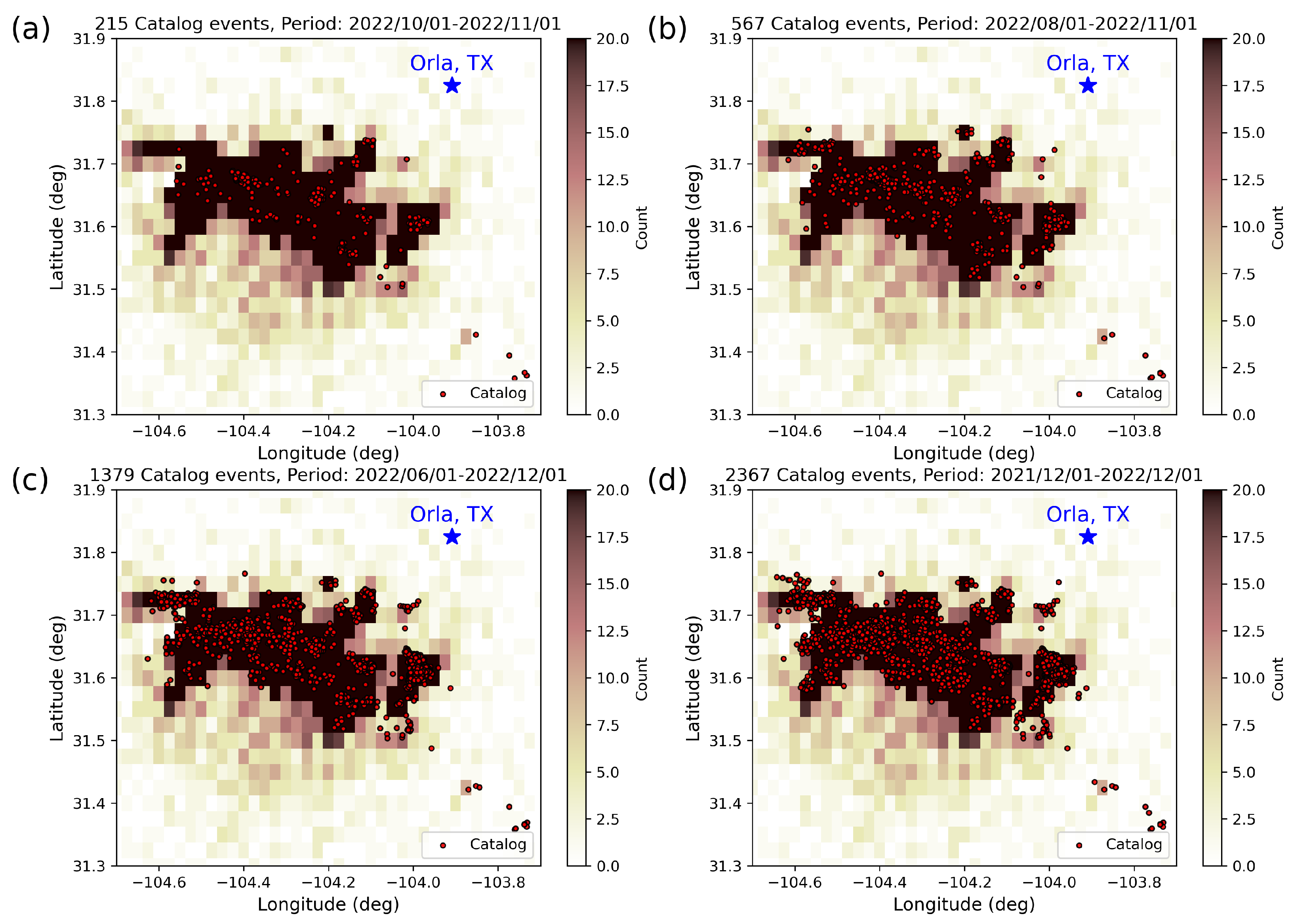
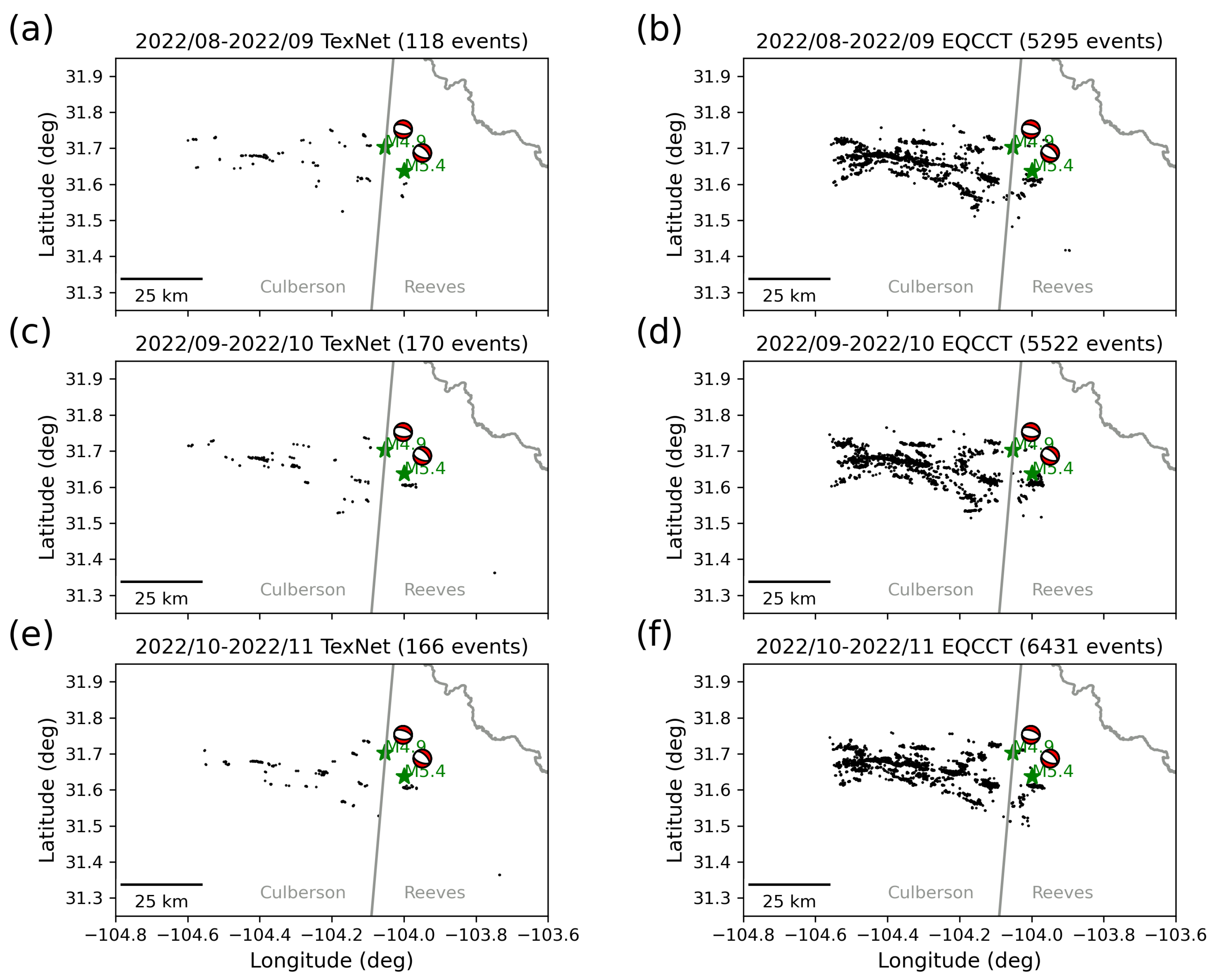
4.1. Event Distribution

Figure 2 shows the density plot of the EQCCT catalog overlapped by the TexNet catalog events of different periods. Figure 2a plots the EQCCT event density overlapped by one month of TexNet events (a total of 215 events). Figure 2b plots the EQCCT event density overlapped by the three-month TexNet catalog (of the same period as the EQCCT catalog). During this three-month period, there are 567 events on the TexNet catalog. Figure 2c plots the EQCCT event density with TexNet events in half a year (1379 events). Figure 2d plots the EQCCT event density with TexNet events in a year (a total of 2367 events from 1 December 2021 to 1 December 2022). Figure 2 shows that despite the short detection period using EQCCT, the number of detected events is significantly larger than the TexNet catalog within the same period. The number of three-month events from EQCCT is even larger (10 times more) than one year of TexNet catalog events. The geographical coverage of the EQCCT events corresponds well with the TexNet catalog’s events in a much longer period, which indicates the fact that the EQCCT catalog can help reveal a much more detailed (in terms of number of relocated events) seismically active structure than the analysts’ catalog in a much shorter period. To verify the quality of the detected events, we calculated the pick residual root mean square (between the theoretical and observed arrival times) for each event. The location approach LocSAT tries to find a location that has the minimum pick residual root mean square. If the root mean square is too large, the location is adjusted and the picks are included or excluded to decrease the root mean square until the optimal solution is obtained. As a result, for the 33,319 events, there were 32,020 events with a root mean square smaller than 1.0, meaning high-quality events; there were 29,017 events with a root mean square smaller than 0.8, meaning very-high-quality events; and there were 20,097 events with a root mean square smaller than 0.5, meaning confidently real events.

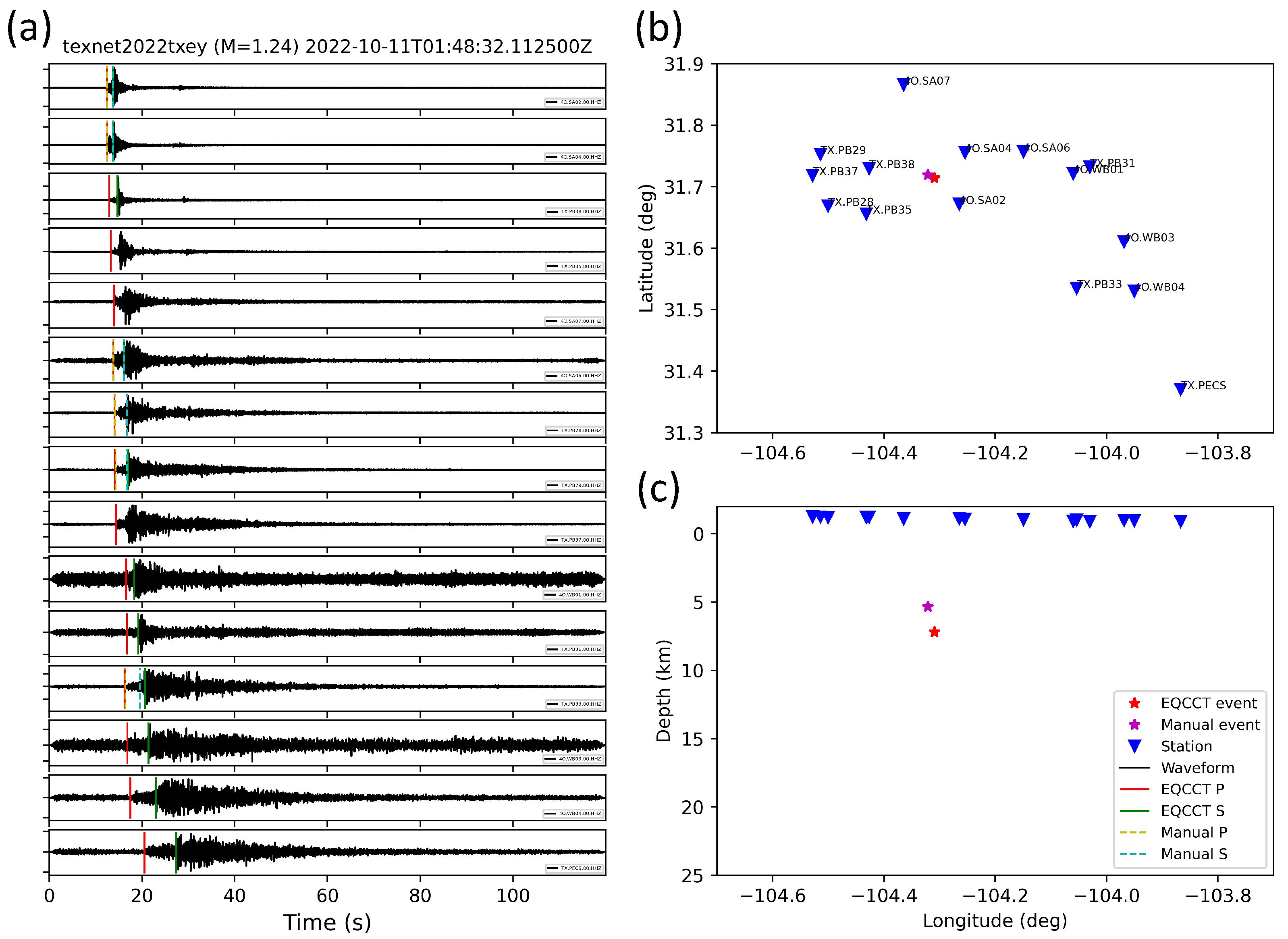
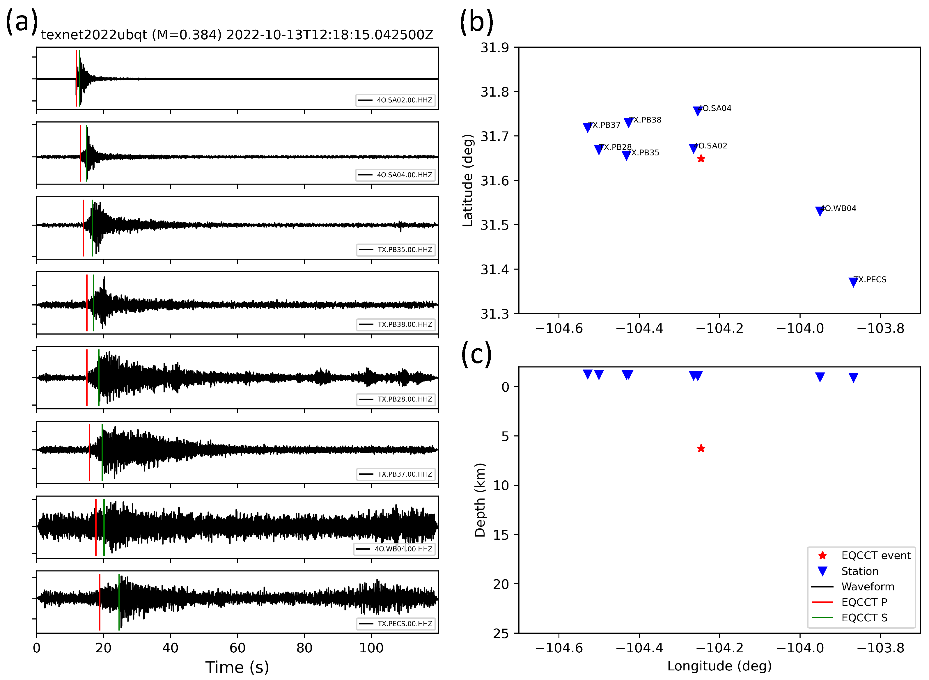
4.2. Picking and Location Examples

For the unprecedentedly large number of events detected per month, it was important to verify the fidelity of these detected events. For large events, the detection results were almost consistent with the TexNet catalog, and their verification was easy, since both EQCCT and analysts were able to detect the events in many stations. The smaller events that were not reported in the TexNet catalog required manual verification. For moderately large events, though they may be captured by the TexNet catalog, EQCCT is typically capable of picking more phases than analysts, especially in cases with low signal-to-noise ratios. Figure 3 plots an example of the detection of the event texnet2022txey. Its magnitude is 1.28 Ml on the TexNet catalog and the magnitude from EQCCT detection is 1.24 Ml. In this example, EQCCT detected this event from 15 stations while analysts detected the event from only 7 stations. The left panel of Figure 3 shows the phase-picking performance using EQCCT or manually. The solid red and green lines mark the EQCCT-picked P- and S-wave arrivals. The dashed yellow and cyan lines mark the manually picked P- and S-wave arrivals. From top to bottom, the epicentral distance increases. The time shown on the top of the left panel is the start time of the segmented 120 s waveforms (10 s before the event origin time). It is clear that at some stations there were only EQCCT picks. In addition, in those stations where both EQCCT and manual picks existed, the two picks were almost the same. The locations and the stations that detected this event are plotted on the right panels of Figure 3. Although the accuracy of the locations determined from the automatic and manual processes requires further validation, the location algorithm can certainly benefit from more detected phases and better constrain the earthquake location.
Figure 4 shows another example of picking and location. In this case, a very small magnitude (Ml = 0.384) event was detected by EQCCT while it was missed by analysts. In this case, the event was detected by eight stations using EQCCT. The location is plotted on the right panels. Considering the distributions of the P- and S-wave picks as the epicentral distance increases, the picks were generally accurate. This example is a demonstration of the capability of the EQCCT method in detecting very small earthquakes.

4.3. Initial and Secondary Location
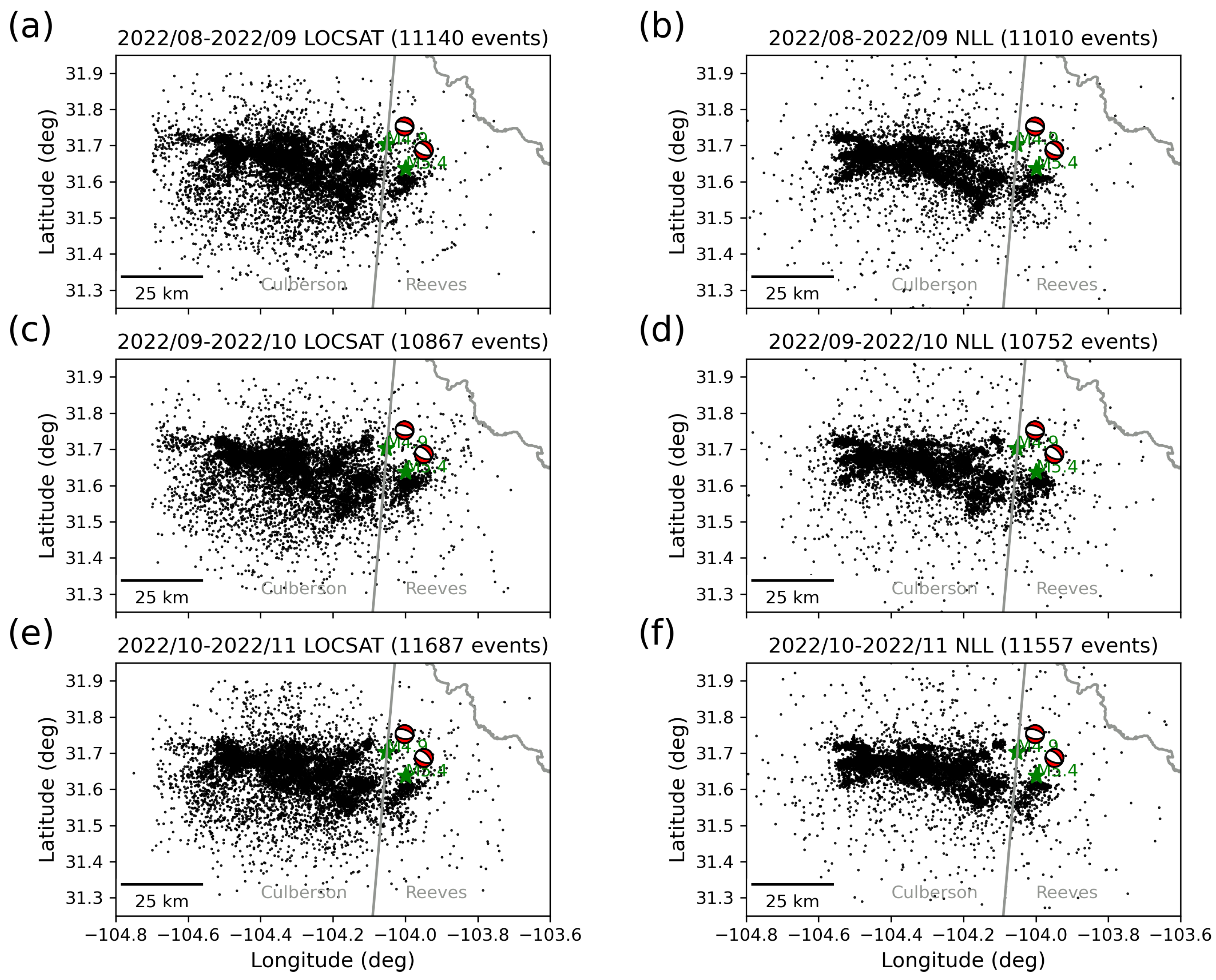
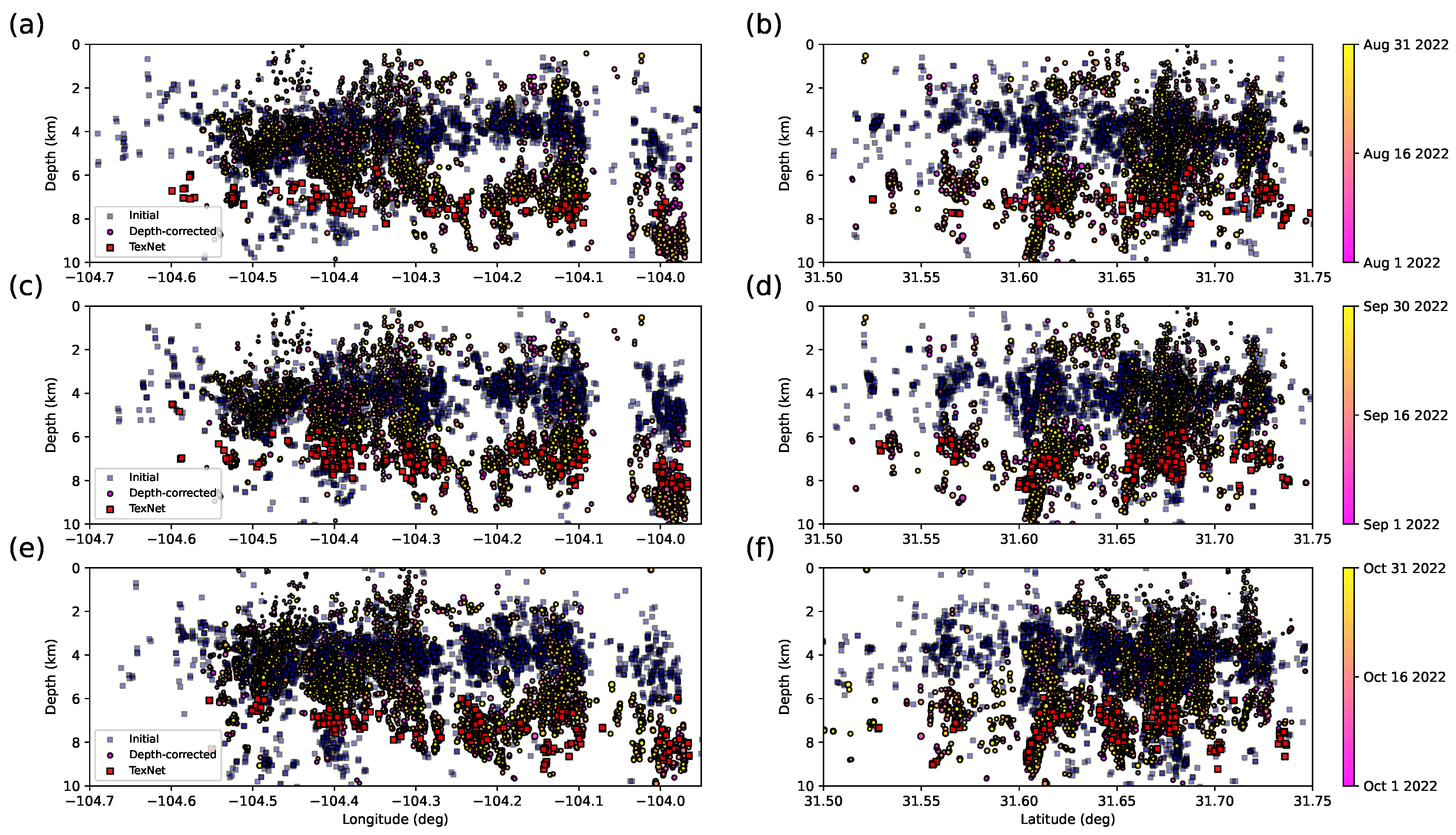
In order to evaluate the effectiveness of the secondary location using NonLinLoc and with a more accurate regional velocity model, we compared the epicenter locations before and after applying NonLinLoc for refined location. To understand the temporal evolution of the earthquake events, we compare the catalogs month by month in Figure 5. In the month of August 2022, the LocSAT method initially associated and located 11,140 events, which was reduced to 11,010 events after NonLinLoc refined the location. In the month of September 2022, the LocSAT method initially associated and located 10,867 events, which was reduced to 10,752 events using NonLinLoc. In the month of October 2022, the LocSAT method initially associated and located 11,687 events, which was reduced to 11,557 events using NonLinLoc. In all three months, the seismicity was more clustered after using NonLinLoc with a more accurate velocity model, indicating a more accurate earthquake catalog. Figure 5 shows that in addition to the depth correction, which will be illustrated later, epicenter correction was also significant, due to a more precise location approach with a more accurate velocity model.

4.4. Relocation

Relocation results heavily depend on the input controlling threshold parameters. In our case, the cross-correlation threshold and the number of good measurements played the most important roles. By using different threshold parameters, we may get different results. Figure 6 shows a test on how the threshold parameter would affect the relocated events. Figure 6a plots the depth-corrected catalog events using NonLinLoc. Figure 6b shows the relocated events with a looser threshold criterion. In this case, the cross-correlation threshold was chosen as 0.35 and the number of good measurements was chosen as 4. As a result, there were 7486 events remaining after the relocation. Figure 6c shows the relocated events with a stricter threshold criterion. In this case, the cross-correlation threshold was chosen as 0.65 and the number of good measurements was chosen as 6. As a result, there were 5758 events remaining after the relocation. The larger number of remaining events using a looser threshold criterion is compromised by the relatively lower resolution of the relocated events. The lower resolution of the relocated events is less effective in delineating the subtle faulting structures with a larger uncertainty.
We also compare the high-resolution relocated events using EQCCT with the relocated events of the TexNet catalog on a monthly basis (Figure 7). The left column of Figure 7 corresponds to the relocated catalog events in August, September, and October 2022, respectively, where only 118, 170, and 166 events were relocated in the three months. The right column of Figure 7 plots the relocated events using EQCCT, where 4853, 4973, 5758 events remained. The comparison between the TexNet relocation catalog and the EQCCT relocation catalog is dramatically different, with the EQCCT catalog containing almost 40 times more events than the TexNet catalog. The monthly relocated catalogs beautifully reveal the active faults in the CMEZ area.
We also compare the depth slices of the relocated events between TexNet, initial, and depth-corrected EQCCT catalogs in Figure 8. The left column in Figure 8 shows the depth-longitude projection slice (all events are projected onto the depth-longitude plane) and the right column in Figure 8 shows the depth-latitude projection slice. Both TexNet and initial EQCCT catalog events are denoted by squares with red and blue colors, respectively. The depth-corrected EQCCT catalog is colored by the origin times and is sized by magnitudes. The comparisons are shown month by month to reveal the temporal evolution of the seismicity. Figure 8 shows clearly that the depth correction using NonLinLoc with the regional velocity models effectively corrects the depth to be consistent with the TexNet catalog events. While the monthly relocation results of the TexNet catalog reveal some subtle lineaments, especially when observing the depth-latitude slices, the EQCCT catalog makes the lineaments highly detailed and clearly unveils the spatial distribution of the basement-rooted and shallow fault structures.

5. Discussion

5.1. Seismotectonic Implications

We first converted Ml (local magnitude) to Mw (moment magnitude) using a scaling law. We then used the converted Mw to establish the magnitude-frequency distribution [37] for the CMEZ, using the EQCCT catalog of 2022/08–2022/10. In addition, in order to compare b-values (an indicator about the causal factor) resulting from different datasets for the same area over time, we determined b-values using TexNet’s catalogs of 2022/08–2022/10 (referred to as TexNet-1) and 2017/01–2022/10 (referred to as TexNet-2), respectively. As expected, we obtained three different b-values out of three different datasets, as shown in Figure 9. Here, we summarize the comparison results.
First, for the same time period (2022/08–2022/10), the EQCCT catalog has a total of 32,480 earthquakes with Mw ranging from −1.9 to 4.1 and presents a normal distribution type. In contrast, the TexNet-1 dataset shows a sparse distribution containing only 535 events with Mw = 0.5 − 4. Clearly, in the EQCCT catalog the number of small earthquakes (Mw < 1.5) has greatly increased. While the b-values resulting from the two datasets are slightly different (1.10 of TexNet-1 vs. 1.13 of EQCCT) their uncertainties differ by nearly 5 times (0.05 of TexNet-1 vs. 0.01 of EQCCT). Meanwhile, the magnitude of completeness, indicated as cut-off Mw in Figure 9, has also significantly reduced from 1.6 to 0.3. We also observed that the lack of smaller earthquakes resulted in a relatively low b-value result from the TexNet-1 dataset.
Secondly, for the TexNet-2 dataset, it presents a much more Gaussian distribution type, as compared to that of TexNet-1, where we have the resulting b-value = 1.17 with uncertainty = 0.02 and magnitude of completeness of 1.6. Given the long time span of this dataset (nearly 6 years), we considered b-value = 1.17 as the background number. A comparison of the b-value between TexNet-2 (1.17) and EQCCT (1.13) suggests that one needs to use a well-distributed catalog to determine a background b-value.
In summary, EQCCT greatly improves detection capability and can further reduce potential artifacts introduced into the b-value due to the incomplete magnitude-frequency distribution. This is a great advantage for evaluating seismic potential using a short time span.

5.2. Spatiotemporal Correlation with Injections

To study spatiotemporal correlation with fluid injection, we selected a target area (highlighted by the yellow circle in Figure 10a) in the CMEZ region. There is much work to be done to obtain a comprehensive correlation analysis between the three-month catalog from this study and the injection activities. Here, we only chose October 2022 as an example to demonstrate the benefits of association with injection well activities using the highly complete seismic catalog. There were only 31 wells operating in CMEZ in October 2022, which are plotted as the diamonds in Figure 10a. We chose a well (well I) that began injection right after the M3.5 event, and we analyzed its association with nearby seismicity. We chose an area centered by the well with a radius of 0.1 deg (highlighted in yellow) to analyze the relationship between injection (8 wells in the yellow circle) and seismicity. We plotted the daily distribution of the number of detected earthquakes in Figure 10b, where we see a generally stable distribution of the number of events but a gradual decrease from 20 October 2022 to 27 October 2022. We plot the magnitude-time distribution in Figure 10c, where the black dots show the TexNet events and the green dots show the EQCCT-detected small earthquakes. We see a sudden drop in the number of small earthquakes on 27 October 2022. We draw the daily injection volumes of the existing wells and the center well (well I) in the CMEZ area in Figure 10d, and a good correlation can be observed between the injection activities and the sudden drop in the number of earthquakes. It is clear that the injection rate peaked on 27 October 2022 while the daily number of earthquakes (mostly small ones) was lowest. Traditionally when we cannot detect so many small earthquakes it is difficult the analyze the influence of the small earthquake activities versus the fluid injection. The moderate-to-large earthquake activities do not show dramatic change during the short-term fluid injection. However, due to the detection of an enormous number of small earthquakes, we can find a distinct drop in the small earthquake activities as the injection rate peaks. This observation is against the mainstream assumption regarding the relationship between fluid injection rate and seismicity. It is commonly thought that increased fluid injection causes increased rates of seismicity; this thinking, however, is contradicted by what we have observed in our study when it comes to ultra-small earthquakes (e.g., Ml < 1). The observation of this study might be explained by the lubricant effect of the fluid in the earthquake-generation mechanism [38]. The fast-injected fluid smooths the faults and reduces the number of small earthquakes in the short term, while the stress is accumulated for subsequent larger earthquakes. It could also be attributed to delayed triggering, which can be explained by rate–state friction laws [39,40]. However, more research needs to be carried out to confirm this hypothesis.

5.3. Future Development

Comparing the catalogs from the NonLinLoc-refined location and the Growclust-based relocation, we find that a significant portion of the detected events are missed in the Growclust-based relocation step. The removal of the large number of events in the original catalog does not necessarily mean that a large portion of the detected events are spurious. It may be partially due to the stringent criterion (the high cross-correlation value and a large number of good measurements) in the Growclust software and is also due to some erroneous picks from the EQCCT picker. Thus, in the near future, on the one hand, we can further investigate the influence of the parameterization or inherent drawbacks of the Growclust software on the final number of retained events. On the other hand, we will keep improving the precision of automatically picked P- and S-wave arrival times using the EQCCT picker. One possible way may be strengthening the current EQCCT model that was trained from global earthquake data by transfer learning on the regional dataset from TexNet. This will hopefully improve detection ability and arrival-picking precision. Concatenation of the highly complete catalog from this study with other data sources, e.g., InSAR data, and pore-pressure simulation data, could give hints on more detailed analysis of how induced earthquakes are generated and how the seismicity is migrating according to the fluid injection in the CMEZ area.

6. Conclusions

We have proposed a robust earthquake-detection-and-location workflow based on the newly developed EQCCT P- and S-wave picker. Thanks to the recently densified broadband seismic stations and EQCCT picker, we have been able to detect and locate thousands of small earthquakes per month in the CMEZ area, most of which were not reported in the public TexNet catalog. The enormous number of small earthquakes helps delineate the subsurface active faults at an unprecedentedly high resolution. The new catalog, especially those ultra-small earthquakes below manual detection ability, reveals a surprising correlation between the occurrence of small earthquakes and the temporally intensified fluid injection rate, which remains to be further explored. This highly complete earthquake catalog arising from deep learning techniques also sheds light on more accurate earthquake forecasting and hazard assessment.

Author Contributions

Conceptualization, Y.C. (Yangkang Chen) and A.S.; methodology, Y.C. (Yangkang Chen) and O.M.S.; software, Y.C. (Yangkang Chen), O.M.S. and D.S.; formal analysis, Y.C. (Yangkang Chen), G.-C.D.H., Y.C. (Yunfeng Chen), S.F., C.B. and I.G.; data curation, Y.C. (Yangkang Chen); writing—original draft preparation, Y.C. (Yangkang Chen); writing—review and editing, all authors; visualization, Y.C. (Yangkang Chen); project administration, Y.C. (Yangkang Chen) and A.S. All authors have read and agreed to the published version of the manuscript.

Funding

Our research was partially supported by research funding granted to the Texas Seismological Network Project, sponsors of the Texas Consortium of Computational Seismology, and starting funds from Zhejiang University.

Data Availability Statement

The online repository of the EQCCT project can be found on GitHub: https://github.com/chenyk1990/eqcct accessed on 20 April 2024. The TexNet waveform data can be accessed through the Data Management Center. The catalog in ASCII form can be downloaded from https://drive.google.com/drive/folders/1lbWHLRHm6aNkZpyHslM2lfZ-nT3_MZat?usp=sharing accessed on 20 April 2024, with the columns denoting eventID, origin time, longitude, latitude, depth, magnitude.

Conflicts of Interest

The authors declare no conflicts of interest.

References

  1. Frohlich, C.; Davis, S.D. Texas Earthquakes; University of Texas Press: Austin, TX, USA, 2003. [Google Scholar]
  2. Frohlich, C.; Hayward, C.; Stump, B.; Potter, E. The Dallas–Fort Worth earthquake sequence: October 2008 through May 2009. Bull. Seismol. Soc. Am. 2011, 101, 327–340. [Google Scholar] [CrossRef]
  3. Justinic, A.H.; Stump, B.; Hayward, C.; Frohlich, C. Analysis of the Cleburne, Texas, earthquake sequence from June 2009 to June 2010. Bull. Seismol. Soc. Am. 2013, 103, 3083–3093. [Google Scholar] [CrossRef]
  4. Frohlich, C.; DeShon, H.; Stump, B.; Hayward, C.; Hornbach, M.; Walter, J.I. A historical review of induced earthquakes in Texas. Seismol. Res. Lett. 2016, 87, 1022–1038. [Google Scholar] [CrossRef]
  5. Fan, Z.; Eichhubl, P.; Gale, J.F. Geomechanical analysis of fluid injection and seismic fault slip for the Mw4. 8 Timpson, Texas, earthquake sequence. J. Geophys. Res. Solid Earth 2016, 121, 2798–2812. [Google Scholar] [CrossRef]
  6. DeShon, H.R.; Hayward, C.T.; Ogwari, P.O.; Quinones, L.; Sufri, O.; Stump, B.; Magnani, M.B. Summary of the North Texas earthquake study seismic networks, 2013–2018. Seismol. Res. Lett. 2019, 90, 387–394. [Google Scholar] [CrossRef]
  7. Skoumal, R.J.; Kaven, J.O.; Barbour, A.J.; Wicks, C.; Brudzinski, M.R.; Cochran, E.S.; Rubinstein, J.L. The induced Mw 5.0 March 2020 west Texas seismic sequence. J. Geophys. Res. Solid Earth 2021, 126, e2020JB020693. [Google Scholar] [CrossRef]
  8. Hennings, P.H.; Young, M.H. The TexNet-CISR collaboration and steps toward understanding induced seismicity in Texas. In Recent Seismicity in the Southern Midcontinent, USA: Scientific, Regulatory, and Industry Responses; Geological Society of America: Boulder, CO, USA, 2023. [Google Scholar] [CrossRef]
  9. Savvaidis, A.; Young, B.; Huang, G.-c.D.; Lomax, A. TexNet: A statewide seismological network in Texas. Seismol. Res. Lett. 2019, 90, 1702–1715. [Google Scholar] [CrossRef]
  10. Doser, D.; Baker, M.; Luo, M.; Marroquin, P.; Ballesteros, L.; Kingwell, J.; Diaz, H.; Kaip, G. The not so simple relationship between seismicity and oil production in the Permian Basin, west Texas. Pure Appl. Geophys. 1992, 139, 481–506. [Google Scholar] [CrossRef]
  11. Frohlich, C.; Hayward, C.; Rosenblit, J.; Aiken, C.; Hennings, P.; Savvaidis, A.; Lemons, C.; Horne, E.; Walter, J.I.; DeShon, H.R. Onset and cause of increased seismic activity near Pecos, West Texas, United States, from observations at the Lajitas TXAR seismic array. J. Geophys. Res. Solid Earth 2020, 125, e2019JB017737. [Google Scholar] [CrossRef]
  12. Grigoratos, I.; Savvaidis, A.; Rathje, E. Distinguishing the causal factors of induced seismicity in the Delaware Basin: Hydraulic fracturing or wastewater disposal? Seismol. Soc. Am. 2022, 93, 2640–2658. [Google Scholar] [CrossRef]
  13. Skoumal, R.J.; Barbour, A.J.; Brudzinski, M.R.; Langenkamp, T.; Kaven, J.O. Induced seismicity in the Delaware basin, Texas. J. Geophys. Res. Solid Earth 2020, 125, e2019JB018558. [Google Scholar] [CrossRef]
  14. Gibbons, S.J.; Ringdal, F. The detection of low magnitude seismic events using array-based waveform correlation. Geophys. J. Int. 2006, 165, 149–166. [Google Scholar] [CrossRef]
  15. Schaff, D.P.; Waldhauser, F. One magnitude unit reduction in detection threshold by cross correlation applied to Parkfield (California) and China seismicity. Bull. Seismol. Soc. Am. 2010, 100, 3224–3238. [Google Scholar] [CrossRef]
  16. Yoon, C.E.; O’Reilly, O.; Bergen, K.J.; Beroza, G.C. Earthquake detection through computationally efficient similarity search. Sci. Adv. 2015, 1, e1501057. [Google Scholar] [CrossRef] [PubMed]
  17. Ross, Z.E.; Trugman, D.T.; Hauksson, E.; Shearer, P.M. Searching for hidden earthquakes in Southern California. Science 2019, 364, 767–771. [Google Scholar] [CrossRef] [PubMed]
  18. Zhu, W.; Beroza, G.C. PhaseNet: A deep-neural-network-based seismic arrival-time picking method. Geophys. J. Int. 2019, 216, 261–273. [Google Scholar] [CrossRef]
  19. Mousavi, S.M.; Ellsworth, W.L.; Zhu, W.; Chuang, L.Y.; Beroza, G.C. Earthquake transformer—An attentive deep-learning model for simultaneous earthquake detection and phase picking. Nat. Commun. 2020, 11, 3952. [Google Scholar] [CrossRef] [PubMed]
  20. Saad, O.M.; Huang, G.; Chen, Y.; Savvaidis, A.; Fomel, S.; Pham, N.; Chen, Y. SCALODEEP: A Highly Generalized Deep Learning Framework for Real-time Earthquake Detection. J. Geophys. Res. Solid Earth 2021, 126, e2020JB021473. [Google Scholar] [CrossRef]
  21. Zhang, M.; Liu, M.; Feng, T.; Wang, R.; Zhu, W. LOC-FLOW: An end-to-end machine learning-based high-precision earthquake location workflow. Seismol. Soc. Am. 2022, 93, 2426–2438. [Google Scholar] [CrossRef]
  22. Zhang, F.; Wang, R.; Chen, Y.; Chen, Y. Spatiotemporal Variations in Earthquake Triggering Mechanisms During Multistage Hydraulic Fracturing in Western Canada. J. Geophys. Res. Solid Earth 2022, 127, e2022JB024744. [Google Scholar] [CrossRef]
  23. Hassani, A.; Walton, S.; Shah, N.; Abuduweili, A.; Li, J.; Shi, H. Escaping the big data paradigm with compact transformers. arXiv 2021, arXiv:2104.05704. [Google Scholar]
  24. Mousavi, S.M.; Sheng, Y.; Zhu, W.; Beroza, G.C. STanford EArthquake Dataset (STEAD): A global data set of seismic signals for AI. IEEE Access 2019, 7, 179464–179476. [Google Scholar] [CrossRef]
  25. Saad, O.M.; Chen, Y.; Siervo, D.; Zhang, F.; Savvaidis, A.; Huang, G.-c.D.; Igonin, N.; Fomel, S.; Chen, Y. EQCCT: A production-ready EarthQuake detection and phase picking method using the Compact Convolutional Transformer. IEEE Trans. Geosci. Remote Sens. 2023, 61, 4507015. [Google Scholar] [CrossRef]
  26. Dosovitskiy, A.; Beyer, L.; Kolesnikov, A.; Weissenborn, D.; Zhai, X.; Unterthiner, T.; Dehghani, M.; Minderer, M.; Heigold, G.; Gelly, S.; et al. An image is worth 16x16 words: Transformers for image recognition at scale. arXiv 2020, arXiv:2010.11929. [Google Scholar]
  27. Ioffe, S.; Szegedy, C. Batch Normalization: Accelerating Deep Network Training by Reducing Internal Covariate Shift. arXiv 2015, arXiv:1502.03167. [Google Scholar]
  28. Srivastava, N.; Hinton, G.; Krizhevsky, A.; Sutskever, I.; Salakhutdinov, R. Dropout: A simple way to prevent neural networks from overfitting. J. Mach. Learn. Res. 2014, 15, 1929–1958. [Google Scholar]
  29. Vaswani, A.; Shazeer, N.; Parmar, N.; Uszkoreit, J.; Jones, L.; Gomez, A.N.; Kaiser, Ł.; Polosukhin, I. Attention is all you need. In Proceedings of the 31st Conference on Neural Information Processing Systems (NIPS 2017), Long Beach, CA, USA, 4–9 December 2017; pp. 5998–6008. [Google Scholar]
  30. Loshchilov, I.; Hutter, F. Sgdr: Stochastic gradient descent with warm restarts. arXiv 2016, arXiv:1608.03983. [Google Scholar]
  31. Rößler, D.; Becker, J.; Ellguth, E.; Herrnkind, S.; Weber, B.; Henneberger, R.; Blanck, H. Cluster-search based monitoring of local earthquakes in SeisComP3. In AGU Fall Meeting Abstracts; NASA: Greenbelt, MD, USA, 2016; Volume 2016, p. S31E-06. [Google Scholar]
  32. Ester, M.; Kriegel, H.P.; Sander, J.; Xu, X. A density-based algorithm for discovering clusters in large spatial databases with noise. In kdd; AAAI Press: Menlo Park, CA, USA, 1996; Volume 96, pp. 226–231. [Google Scholar]
  33. Bratt, S.; Nagy, W. The LocSAT Program; Science Applications International Corporation: San Diego, CA, USA, 1991. [Google Scholar]
  34. Lomax, A.; Virieux, J.; Volant, P.; Berge-Thierry, C. Probabilistic earthquake location in 3D and layered models: Introduction of a Metropolis-Gibbs method and comparison with linear locations. In Advances in Seismic Event Location; Springer: Berlin/Heidelberg, Germany, 2000; pp. 101–134. [Google Scholar]
  35. Lomax, A.; Michelini, A.; Curtis, A.; Meyers, R. Earthquake location, direct, global-search methods. Encycl. Complex. Syst. Sci. 2009, 5, 2449–2473. [Google Scholar]
  36. Trugman, D.T.; Shearer, P.M. GrowClust: A hierarchical clustering algorithm for relative earthquake relocation, with application to the Spanish Springs and Sheldon, Nevada, earthquake sequences. Seismol. Res. Lett. 2017, 88, 379–391. [Google Scholar] [CrossRef]
  37. Gutenberg, B.; Richter, C.F. Frequency of earthquakes in California. Bull. Seismol. Soc. Am. 1944, 34, 185–188. [Google Scholar] [CrossRef]
  38. Becken, M.; Ritter, O.; Bedrosian, P.A.; Weckmann, U. Correlation between deep fluids, tremor and creep along the central San Andreas fault. Nature 2011, 480, 87–90. [Google Scholar] [CrossRef] [PubMed]
  39. Segall, P.; Lu, S. Injection-induced seismicity: Poroelastic and earthquake nucleation effects. J. Geophys. Res. Solid Earth 2015, 120, 5082–5103. [Google Scholar] [CrossRef]
  40. Heimisson, E.R.; Smith, J.D.; Avouac, J.P.; Bourne, S.J. Coulomb threshold rate-and-state model for fault reactivation: Application to induced seismicity at Groningen. Geophys. J. Int. 2022, 228, 2061–2072. [Google Scholar] [CrossRef]
Figure 1. Distribution of the events: (a) Map of the Texas seismological network. CMEZ denotes the Culberson and Mentone seismic zone, which is the most seismically active area in Texas. In 2022, 80.85% of Texas seismicity was located in the CMEZ. (b) Stations used in the detection and location. (c) Magnitude distribution. (d) Depth distribution. (e) Distribution of earthquakes by date; each bin represents three days. The reported events represent those events that are detected by the traditional automatic picker short-term average/long-term average at TexNet but are not manually reviewed.
Geosciences 14 00114 g001
Figure 2. Detection and location results (33,319 events) of EQCCT compared with TexNet events in different periods: (a) Location comparison between EQCCT events and one-month catalog events. (b) Location comparison between EQCCT events and three-month catalog events. (c) Location comparison between EQCCT events and six-month catalog events. (d) Location comparison between EQCCT events and one-year catalog events.
Geosciences 14 00114 g002
Figure 3. Pick verification on the event texnet2022txey (1.24 Ml by EQCCT and 1.28 Ml by analysts), which was detected by both analysts and EQCCT: (a) Waveforms. From top to bottom, the epicentral distance increases. The time shown on the top of the waveforms is the start time of the segmented 120 s waveforms (10 s before the event origin time). The red and green lines mark the EQCCT-picked P- and S-wave arrivals. The dashed yellow and cyan lines mark the manually picked P and S arrivals. (b) Station and event locations on the map. (c) Station and event locations on the depth slice. The magenta and red stars mark the manual and EQCCT event locations. In this case, the event was detected by 15 stations using EQCCT while only detected by 7 stations originally by analysts.
Geosciences 14 00114 g003
Figure 4. Pick verification on the event texnet2022ubqt (0.384 Ml), which was detected only by EQCCT and is not in the TexNet catalog: (a) Waveforms. From top to bottom, the epicentral distance increases. The time shown on the top of the waveforms is the start time of the segmented 120 s waveforms (10 s before the event origin time). The red and green lines mark the EQCCT-picked P- and S-wave arrivals. (b) Station and event locations on the map. (c) Station and event locations on the depth slice. In this case, the event was detected by eight stations using EQCCT. Due to the small magnitude and relatively low signal-to-noise ratio of the waveforms, this event was almost impossible to detect by analysts.
Geosciences 14 00114 g004
Figure 5. Comparison between the initial (a,c,e) and refined catalogs (b,d,f) in three months. It is clear that the NonLinLoc location with a regional 1D velocity significantly improved the clustering of seismicity.
Geosciences 14 00114 g005
Figure 6. Comparison of location and relocation results using the catalog that contains 11,557 events detected using EQCCT in October 2022: (a) Input catalog from EQCCT and NonLinLoc. (b) Relocated catalog with a looser threshold. (c) Relocated catalog with a stricter threshold.
Geosciences 14 00114 g006
Figure 7. Single-month comparison of relocation results between the TexNet catalog and the EQCCT catalog: (a) Relocated TexNet catalog between 2022/08 and 2022/09. (b) Relocated EQCCT catalog between 2022/08 and 2022/09. (c) Relocated TexNet catalog between 2022/09 and 2022/10. (d) Relocated EQCCT catalog between 2022/09 and 2022/10. (e) Relocated TexNet catalog between 2022/10 and 2022/11. (f) Relocated EQCCT catalog between 2022/10 and 2022/11.
Geosciences 14 00114 g007
Figure 8. Single-month comparison of relocation results between the TexNet catalog, initial, and depth-corrected EQCCT catalog. Blue squares are relocated initial catalog. Red squares are relocated TexNet catalog. Circles are relocated depth-corrected catalog, which are color-coded by origin times: (a) Relocated catalog in the longitude-depth slice between 2022/08 and 2022/09. (b) Relocated catalog in the latitude-depth slice between 2022/08 and 2022/09. (c) Relocated catalog in the longitude-depth slice between 2022/09 and 2022/10. (d) Relocated catalog in the latitude-depth slice between 2022/09 and 2022/10. (e) Relocated catalog in the longitude-depth slice between 2022/10 and 2022/11. (f) Relocated catalog in the latitude-depth slice between 2022/10 and 2022/11.
Geosciences 14 00114 g008
Figure 9. Frequency-magnitude plots in different cases: (a) Calculated b-value and magnitude of completeness (cut-off Mw) using the three-month TexNet catalog (TexNet-1). (b) Calculated b-value and magnitude of completeness (cut-off Mw) using the whole 6-year TexNet catalog (TexNet-2). (c) Calculated b-value and magnitude of completeness (cut-off Mw) using the three-month EQCCT catalog.
Geosciences 14 00114 g009
Figure 10. Association of seismicity with fluid injection: (a) Spatial distribution of the detected events in October 2022. (b) Daily distribution of the events. (c) Daily magnitude distribution. (d) Daily injected volumes of all wells in the target area (yellow circle in (a)) and the center well.
Geosciences 14 00114 g010
Disclaimer/Publisher’s Note: The statements, opinions and data contained in all publications are solely those of the individual author(s) and contributor(s) and not of MDPI and/or the editor(s). MDPI and/or the editor(s) disclaim responsibility for any injury to people or property resulting from any ideas, methods, instructions or products referred to in the content.

