The Use of High-Resolution Historical Images to Analyse the Leopard Pattern in the Arid Area of La Alta Guajira, Colombia


1
Santiago de Cali University, Calle 5 #62-00 Cali, Valle del Cauca, Colombia
2
Landscape Laboratory, Geography Department, University of Girona, Plaça Ferrater i Mora 1, 17071 Girona, Spain
*
Author to whom correspondence should be addressed.
Geosciences 2018, 8(10), 366; https://doi.org/10.3390/geosciences8100366
Submission received: 24 August 2018
/
Revised: 11 September 2018
/
Accepted: 27 September 2018
/
Published: 29 September 2018
(This article belongs to the Section Biogeosciences)
Abstract
:A recent review of global arid areas supports the idea that there are two patterns to vegetation in arid lands. Patches of thick vegetation alternate with those with much less vegetation or none at all. There is a specific size, shape and spatial distribution that characterizes vegetation patterns in arid land ecosystems. In some places, the patches have irregular shapes; these are called spots or Leopard bush. This research project is based on a biophysical approach that integrates information collected in the field, high resolution historical satellite images and Geographical Information System technology. The results revealed that there were certain places in the landscape that facilitate the singular development of the vegetation. The Leopard pattern results from the interaction of various factors (fertility island, fragmentation of vegetation, anthropic influence, herbivorism). Specific characteristics that limit plant life forms are found in the area; since only certain resistant species develop, these form associations and in turn generate strategies to optimize resources. Eventually, this equilibrium is disturbed by human activities in the shape of ungulate livestock breeding and anthropogenic activities, resulting in a heterogeneity of soils and vegetation whose interaction generates the pattern.
1. Introduction
Dry lands cover approximately 41% of the earth’s land surface, and are home to over 2000 million people (some 35% of the global population) [1]; in Colombia, the percentage is 16.9% [2]. A notable example of dry land in Colombia is found in La Guajira Department, in the northernmost part of both the country and South America. Its location in the Caribbean leads its arid areas to be classified in the country’s bio-geographic provinces as a dry pre-Caribbean belt. The area’s vegetation consists typically of small trees, rigid stunted perennial bushes, and thorny shrubs. The area is primarily inhabited by the indigenous communities who settled there some 5000 years ago, and have adapted to the harsh surroundings [3]. The peninsula’s climate is characterized by the lack of thermal seasons, strong winds, irregular precipitation, and temperatures that can reach highs of between 28 and 33 °C [4].
Over the last two decades, a number of authors [5,6,7] have supported the idea that vegetation in those ecosystems where water is very limited is not continuous, but homogenously organized in two phases, with densely-vegetated patches alternating with patches of little or no vegetation. Over the past 50 years, the planet’s arid and semi-arid areas [8] have shown regional and local spatial forms with vegetation forming regular patterns [9,10,11]. Such patterns are particularly visible from remote sensors. Some ecosystems show the presence of dense patches which form a stripe pattern, also known as the “Tiger Bush pattern”, while, in others the dense vegetation is more patchy; this is called the “Leopard bush pattern” [5]. The tiger bush pattern has patches of vegetation in strips or stripes that alternate with bare, or sparsely covered, ground; these may be between 30 and 400 m long, and 10 to 50 m wide. The leopard bush pattern has patches of vegetation in spots, or ground cover alternating with bare ground; these can be from 1 to 10 m long, and 2 to 50 m wide (Figure 1). It has been hard to reach a theoretical definition for these patterns, as well as other regular patterns that are called “Maze patterns”, which are frequently seen in North American and Eurasian wetlands. However, most hypotheses link such features to a range of causes; the selective grazing of herbivores; the effects of fire; anisotropic environmental conditions; seed dispersal over long and short distances; and competition between plant species [7]. According Lejeune et al. [12], aperiodic and isolated vegetation patches observed in South America and West Africa are interpreted as localized structures arising from the coexistence between the bare state and the patchy vegetation state. The same mechanism has been applied to gaps of vegetation such as fairy circles in Namibia [13,14] and to the patches of vegetation observed in the Sajama National Park in Bolivia [15]. Also, the transition from periodic distribution of patches of vegetation to tiger bush type of pattern [16].
Patches of vegetation usually have a characteristic size and well defined circular shape in isotropic environmental conditions. However, It has been shown recently that patches can be destabilized by a deformation of their circular shape, either leading to the formation of labyrinthine patterns (Tiger bush), or dividing into two new identical patches of smaller diameter. This mechanism, called a self-replication of localized vegetation patches in arid or semi-arid-ecosystems has been proposed to explain the spatially periodic distribution of vegetation patterns in herbaceous populations of the Catamarca region, Argentina [17] and in Zambia and Mozambique [18]. The analysis is based on both remote sensing analysis (statistical analysis of satellite images) and the mathematical modeling using a generic interaction-redistribution model, based on the relationship between the structure of individual plants and the facilitation-competition interactions existing within plant communities. A review of published research shows that, while the tiger pattern has been widely studied in the semi-arid regions of Africa, Asia, Australia and North America, the leopard pattern has been the subject of little research (Table 1). Analyses of this latter have mainly been through the use of numerical simulations [19].
This research developed a biophysical approach that integrated Geographical Information System (GIS), Remote Sensing (RS), and information gathered in the field to isolate the specific environmental conditions of La Guajira that cause such patterns. Such tools provide the data from which geospatial models can be implemented. These, along with first-hand information, aid in understanding the behaviour of the vegetation patches. High-resolution satellite images were used to analyze the fragmentation and land use; some of these were historical (Corona KH-4A), and some contemporary (Quick Bird, EROS-B). Elevation models were also used in the preprocessing step and geomorphological interpretation. Fundamental features of the leopard pattern are the fragmentation of vegetation cover, and the distances between them; satellite images provide information regarding the relation between the variables that play a role in the development and distribution of the vegetation pattern. It is posited that the distribution and composition of the Leopard pattern in the Guajira Peninsula originates from the interaction between anthropic and environmental aspects, which facilitate the singular development of the vegetation. Specific characteristics that limit plant life forms are found in the area; these in turn generate strategies to optimize resources and are eventually disturbed by ungulate livestock breeding and anthropogenic activities, resulting in a heterogeneity of soils and vegetation generated by this disturbance.
2. Materials and Methods
2.1. Study Area
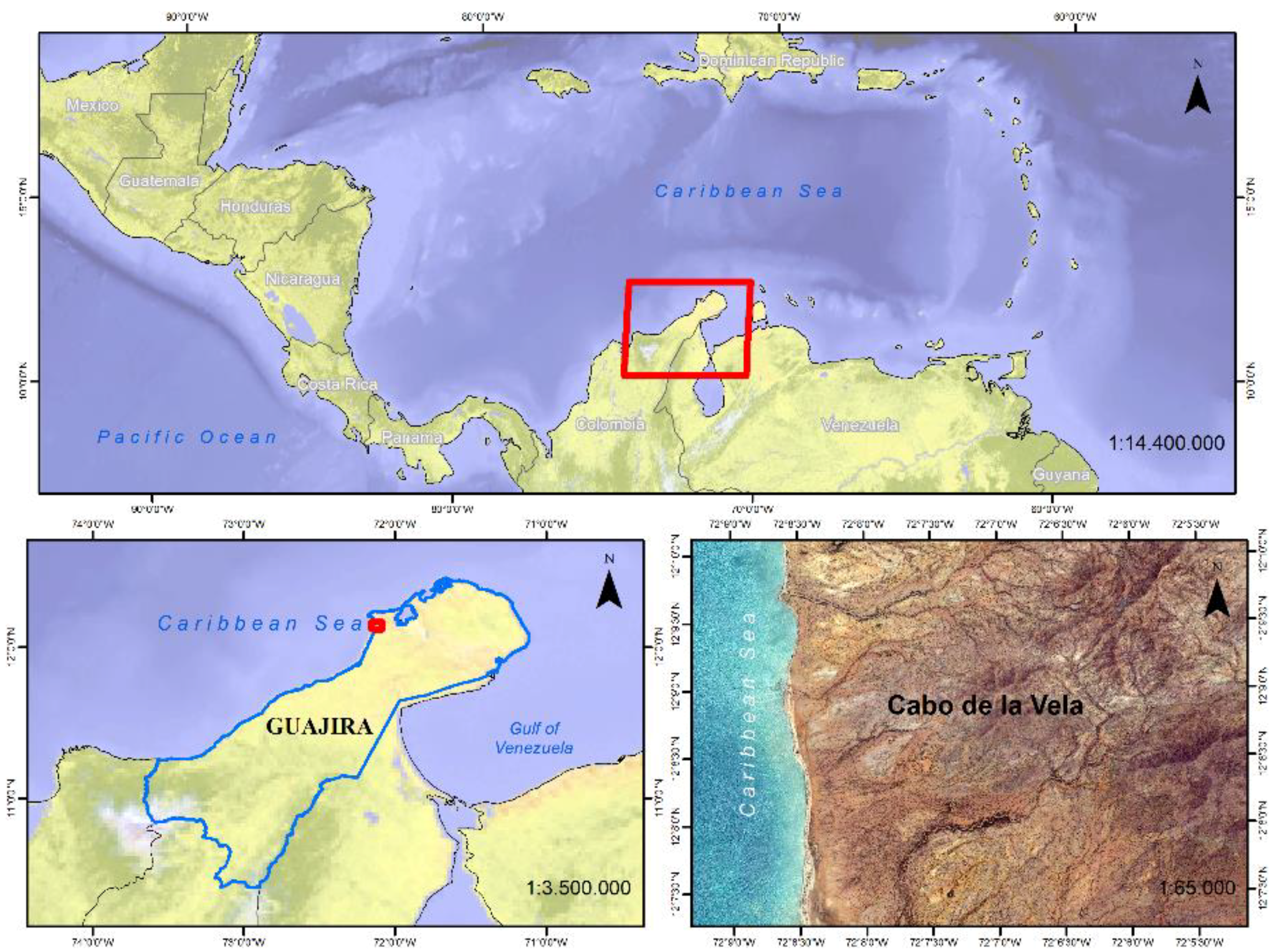
The peninsula of La Guajira is in northern Colombia and Venezuela, and is surrounded by the Caribbean Sea; it has an area of some 6800 km2, and is located in the northernmost part of South America (Figure 2). The Colombian part of the peninsula is called the Alta Guajira; it has large flat areas, and some small mountain ranges, the highest point being 867 m. The research was carried out in a square area in the Cabo de la Vela municipality (Figure 2). Most of the land in the study area is flat, although there are a number of mountain ranges and small hills, the highest of which reach 200 m. All the area’s inhabitants belong to indigenous communities; their livelihood is mostly gained from goat and sheep farming, and fishing from the adjacent shore. It has an area of some 43 km2, it lies between 12°8’54.92” N, 72°7’18.76” W and 12°7’12.85” N, 72°7’18.57” W. The departmental capital, Riohacha, is 120 km away, and the Colombian capital 900 km [32].
2.2. Satellite Images
2.2.1. Corona KH-4A Images
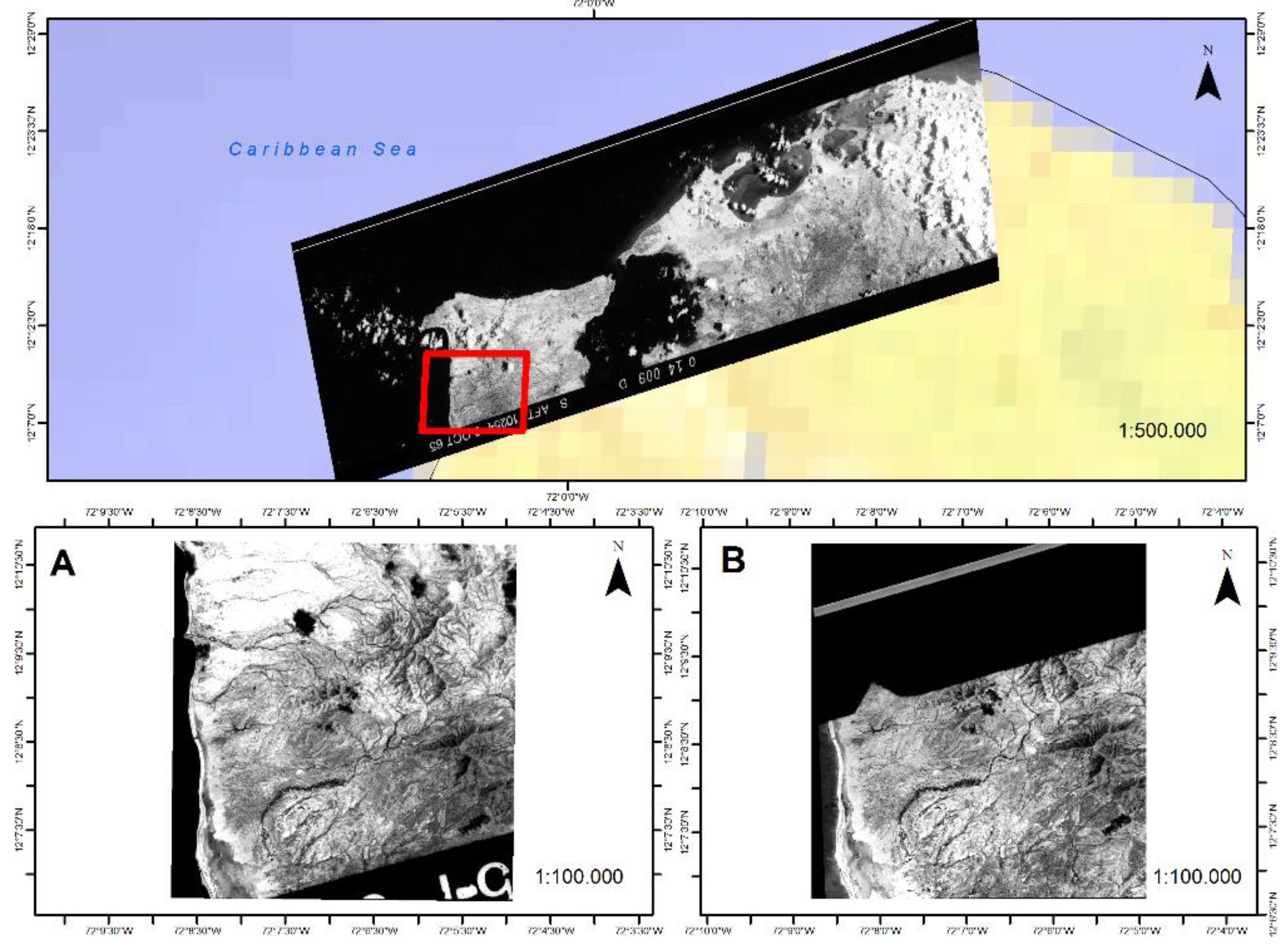
Corona KH-4A was one of a group of spy satellites operated by the CIA. The programme ran from the early years of the Cold War, in 1960, and ended in 1972. These were the first high-resolution satellites, and Corona KH-4A was launched in August 1960 [33]. Corona’s images were panchromatic satellite photographs recorded on film, with a visible spectrum response (400–700 nm). The photographs were taken using a panoramic camera that recorded the images onto a roll of film [34]; exposed film was then jettisoned and recovered in the air by specially designed aeroplanes [35]. Each Corona KH4A mission photograph covers some 17 by 232 km. Data was digitalized in four superimposed files, separated to an 8-bit radiometric accuracy with a single panchromatic band [35]. The full archive of Corona images was declassified in 1995; it has been fully indexed and can be downloaded from the United States Geological Service (USGS) at a nominal ground resolution of between 2.74 and 1.83 m. This research used two Corona KH-4A sensor images from 6 October 1965 ID DS1025-1014DA009 and DS1025-1014DA010 (Figure 3), processed to a standard PAN-type quality. They were obtained from the USGS via the Earth Explorer system https://earthexplorer.usgs.gov/.
In recent years, the great potential of these declassified images can be seen in some of the scientific studies that used Corona images (Table 2).
2.2.2. Quick Bird Images
QuickBird is a commercial high-resolution satellite operated by DigitalGlobe, put into orbit on 18 October 2001 from the Vandenberg air base, USA. This satellite is able to acquire information with a sub metric accuracy of 0.61 cm in panchromatic 450–900 nm mode, and of 2.44 m in four multispectral bands; blue (450–520 nm); red (520–600 nm); green (630–690 nm); and near infrared (760–900 nm). It orbits at a height of 450 km, synchronously with the sun every 93.5 min. Above the equator, its inclination is 97.2°, and 16.5 km at the nadir (the closest point to the satellite, which generally coincides with the center of the image). It has an on-board storage capacity of 160 GB. An archive image dating from 15 March 2007 ID 1010010005867100 was used (Figure 4).
2.2.3. Eros B Images
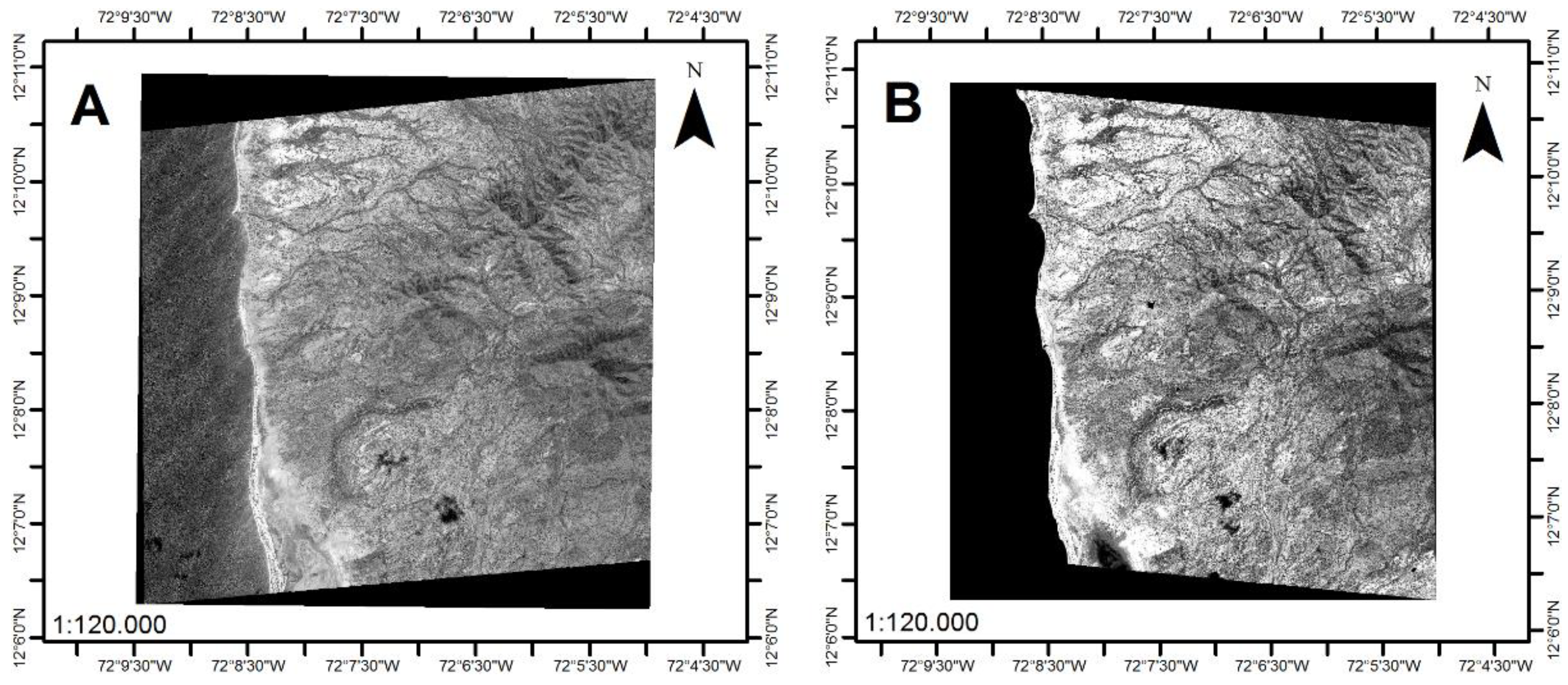
Eros B is a high-resolution Israeli satellite operated by ImageSat International. It was launched on 25 April 2006 from the Svobodny launch complex in Siberia, Russia. The satellite can gather information with sub metric accuracy from a Push-broom type CCD-TDI sensor to acquire a panchromatic band (500–900 nm) with a spatial resolution of 70 cm at the panchromatic and it is capable of obtaining stereoscopic images in two adjacent orbits. The satellite’s stereoscopy is fundamental when obtaining ground elevation. The images have a stereoscopic effect since they are of two fields of view, these may be across and along the satellite’s track. The images are of two close but slightly different orbits; one is taken from an angle of between 60° and 75°, while the other is taken from an oblique angle of the satellite’s path, of between 60° and 97.4°. This shows that the satellite can turn in relation to its orbit (Figure 5). Satellite sensors with this feature can be termed stereoscopic image systems since the data they provide can be used to calculate three-dimensional coordinates, producing information regarding ground height. Two stereo images of the lower La Guajira area were taken on request in 6 February 2013 ID MBT1-e2376518 and MBT1-e2376519.
2.3. Modelling of Sensor Parameters
The topographic data available of the area studied dates from the early 1970s; however, they show very little detail, and are now out of date. In order to reconstruct a topographical digital surface model (DSM), stereoscopic pairs of high-resolution satellite images taken from the EROS B platform were used. DSMs are the true representation of all of the variations in elevation of the objects and surfaces present at the time of data collection. The main difference between DTMs and DSMs is that the former represent only the elevation values of the lowest points of a surface (terrain), whereas the latter represent the elevation of the surface layer of objects on the terrain. DTMs can be a product of a DSM process. This process was considered to be a practical and cost-effective alternative methodology. DSM is a layer of information that is useful in the orthorectification process of satellite images once they have been classified. The study used the OrthoEngine module of the PCI Geomatic photogrammetric computer programme to generate a DSM; and Rational Polynomial Coefficients were extracted. An analysis scale of 1:10,000 was defined for the study area. Two CCD EROS-B sensor images were used with an L1A processing level. The meta-data of two EROS B stereo images of Cabo de la Vela with different angles of view produced the satellite orbit, control, and altitude data. Ground Control Points taken on the ground for both images were entered; the Tie Points (points located in two geographically superimposed raster images); and the Check Points in each image were measured. A mathematical model was created associated to the satellite’s position for both stereoscopic images through the manipulation of orbit and height data with the control point data; the root mean square was then used to analyze the point error (Table 3). One-hundred-and-fifty control points, 80 tie points, and 20 check points were taken.
2.4. Generation of DSM and DTM
The first fundamental step in creating the DSM was the calculation of the epipolar image for one of the images. This showed that both images are compensated in the X parallax. A pixel in the original image was located using statistical functions calculated for the overlapping area of the images (Parallax). The height of a specific point can be calculated through the use of the average, final value, or highest correlation of the pixel parallax. The next stage was the generation of the DSM with a resolution of 2 m; any areas that provided no information regarding elevation, or had been wrongly calculated were edited out. An image enhancement tool was also used that included the complex processes of interpolation, filtering and image softening, and a masking function to replace filtered values. In photogrammetry, the processes that result from the calculation of the parallax between two images produce the areas of all those objects present when the data was taken. The 3D reconstruction of the area corresponding to the view of the first facet of the ground contains both micro-relief (buildings, trees, etc.), and bare ground. In this case, the choice was made to use a simple data cleaning technique with the DSM2DTM function of the PCI Geomatic programme converting a raster digital surface model (DSM or elevation) into a bare-earth digital terrain model (DTM). Filters are used to remove surface items such as buildings and trees. This process eliminated areas that included houses and small changes in height of those objects present in the data (Figure 6).
The assessment of the quality of DSM and DTMs is generally through the measurement of the RMS between the elevation given by the model and precise measurements of known points. In this case, the analysis produced an acceptable degree of accuracy, with an average margin of error of 1.77 m for the superimposed area, compared with the ground points taken by a sub metric GPS. Bearing in mind that the area was analyzed at a scale of 1:10,000, the DTM that resulted from the DSM cleaning process produced an area with a 2 m margin of error when statistically compared with altimetric field data. The resulting elevation was reliable since the mean square error was under the minimum acceptable level for the 1:10,000 scale, some 8.5 m (Table 4).
2.5. Correction and Orthorectification
Radiometric correction is required in order to correct a number of errors in the sensor that, on interacting with the atmosphere, produce erroneous values, altering the radiance values the satellite receives. This process eliminates the distortions that reach the sensor from the earth’s surface. The QuickBird satellite image from 2007 was acquired at a 2A processing level, showing 0% cloud cover and a prior radiometric correction level from the satellite. The 2013 Eros B satellite image also showed 0% cloud cover and had prior radiometric corrections; since the processing level was also 2A, neither image had banding, pixels or lines lost. The next image analyzed in search of possible deficiencies was the oldest, that from Corona in 1965. These images are not digital, but the result of a high-resolution scan of the film itself, this made it impossible to carry out any radiometric correction. Nonetheless, image quality is good, and shows 1% cloud cover in the analyzed area. In general, satellite images can be processed at different levels. Level 0 is the raw, unprocessed image; level 1A includes radiometric corrections; level 1B has geometric corrections of systematic distortions in the image geometrics, such as poorly aligned scan lines and non-uniform pixel size; and level 2A makes a geometric correction placing the pixels in the geographical space, thus correcting possible standard cartographic projection distortions based on a prediction of the satellite’s position when the image was taken. As previously mentioned, the most modern Eros B and QuickBird images are of level 2A, with a fairly precise location over the ground. Thus, they differ from the Corona image, which provides no reference and is classified as raw, unprocessed level 0. Having two level 2A images therefore makes it possible to take the assigned reference system and use it in this stage of the process. The raw image can be georeferenced using the information provided by the above-mentioned 2A images since the definitive control points needed to make precise geometric corrections of all images were compiled in the field. This process involved the transformation of the pixels in the second image (Corona) so that they precisely coincided with those of the first (Eros B). This was done through a second degree polynomial transformation obtained through a group of pairs of control points of both images. After georeferencing the images, the final geometric correction was made, this was the correction of the topographical effect on the satellite images. This procedure corrects those movements caused by the inclination of the sensor, ground relief, and the curvature of the Earth. The main input in this stage was the elevation model resulting from the DSM process, the specific sensor data when the image was taken (metadata), and control points taken in the field.
2.6. Image Segmentation and Classification
Segmentation is the process by which an image is divided into segments with similar spectral, spatial and/or textural characteristics. Ideally, the image segments correspond to features in the real world. The ENVI programme was used for image segmentation. ENVI (the Enviroment for Visualizing Images) is a revolutionary image processing system. From its inception, ENVI was designed to address the numerous and specific needs of those who regularly use satellite and aircraft remote sensing data. ENVI provides comprehensive data visualization and analysis for images of any size and any type—all from within an innovative and user-friendly environment [47]. It contains a feature extraction module, which uses a methodology that is a hybrid between pixel-based and segment-based classification. Feature extraction uses a focus based on objects in order to classify images, where an object (also called a segment) is a group of pixels with a similar spectrum and/or textural characteristics. The Rule Based Feature Extraction Workflow function was used to create an image of segments for each satellite. The Object Creation module saw the interactive development of the training sites based on the scale and fusion level of each segment. Workflow divides an image into a number of segments and calculates their various attributes; then rules are constructed to classify those features of interest. Each rule contains one or more attributes, such as area, length, or texture, which are restricted to a specific range of values. In the Rule Base model, a parametric rule classifier was used based on the interactive classification of the histogram of each segment in order to isolate the three classes defined above. Finally, the classifications were exported in the ArcGis Shape vector format.
3. Results
3.1. Land Use and Cover Maps
Three types of high-resolution satellite images were used in the research, the aim being to obtain the most detailed information on vegetation cover in those years when high resolution was accessible (1965, 2007, and 2013). The legend used to classify ground cover at a 1:10,000 scale was based on the fact that patterns in arid areas are produced by only a few plant species; thus, only three classifying groups are used (Table 5). In producing those classes related to land use, geometric entities were generated from the coverage layers to be independently analyzed.
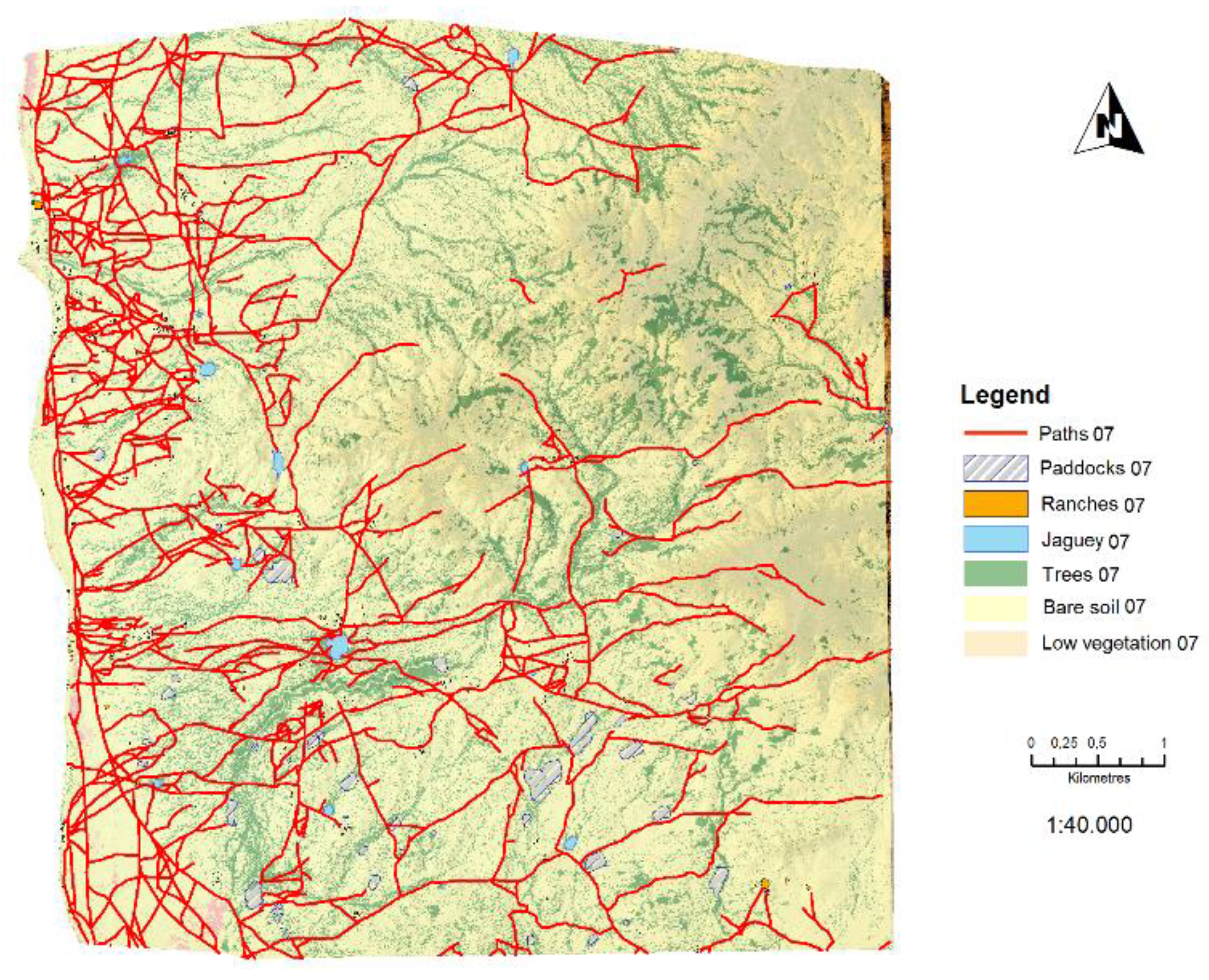
The coverage maps (1965, 2007 and 2013) were the result of applying the attributes table to differentiate the required classes. The segmentation process provided great detail on the coverage present in the area. Land use characteristics, such as paths, ranches, jaguey and paddocks were digitalized manually for each of the years (Figure 7, Figure 8 and Figure 9). The Kappa coefficient is a statistical measure that adjusts the effect of chance on the proportion of the observed agreement for qualitative elements where P(A) is the proportion of times that the coders agree and P(E) is the proportion of times that we would expect them to agree by chance [48].
The kappa coefficient was used to carry out a statistical evolution of the maps; it is one of the most widely used in assessing classification process results, or the visual interpretation of satellite images [49]. The advantage of this coefficient is that it estimates the classification errors in each of the classes; that is, it is a weighted value of the complete quality of the classification that is closest to reality [50]. The kappa value is obtained through a confusion matrix that tabulates the number of correct and incorrect elements in the classification. In order to determine the truth on the ground, a random distribution of points is made, taking into account the total area studied and finding the category deemed correct at each point. Confusion matrix reference values must be the truth on the ground, which is set out in the columns, while the classification values are in the rows. Confusion matrix results were 0.9312 for 2013; 0.9521 for 2007; and 0.9165 for 1965. These results are high due to the few classes and the level of detail obtained of ground cover during the segmentation process. The satellite images enabled the classification of paths, infrastructure, and jaguey present in each of the images. Vectors were delineated and polygons created using the ArcGis programme computational view. Results for 1965 showed 69.01 km of paths, with 44.06 Ha of paddocks, 1.37 Ha of ranches, and 2.25 Ha of water. Results for 2007 showed 229.68 km of paths, 34.81 Ha of paddocks, 3.87 Ha of ranches, and 8.49 Ha of water. Results for 2013 showed 324.50 km of paths, 31.57 Ha of paddocks, 7.13 Ha of ranches, and 13 Ha of water. The evolution of the main aspects of land use shows a clear rise in anthropogenic features that directly affect the landscape. Paths increased from 69.01 km in 1965 to 324.5 km in 2013, ranches from 1.37 Ha in 1965 to 7.13 Ha of built area in 2013, their number rising from 130 to 695 over the 1965–2013 period. Jagüeys rose from 2.5 Ha in 1965 to 13 Ha in 2013. The period saw a rise in size, distance, and quantity in almost all aspects. The only aspect that showed a fall was the area occupied by paddocks, which fell from 44 Ha in 1965 to 31.57 Ha in 2013. Nonetheless, the number of paddocks continues to rise; in 1965 there were 46 paddocks, with an average area of 9579 m2, while in 2013 there were 180, with an average area of 1816 m2.
3.2. Landscape Units and Plant Formations
The climatic aspect is the first classifier of the landscape identified as hyper arid in the area. The average temperature of the area was 28.45 °C, with the highest temperatures being in June, July and August. The average precipitation for the area was 27.82 mm, October being the wettest with 100.41 mm and February the least wet with 1.41 mm. A climograph representing precipitations and temperatures for the area shows that the precipitations are lower than the average temperature for almost all months except October (wet period). The climograph indicates that it is an arid area according to the De Martonne index, the rainfall curve being below the temperature curve 11 out of 12 months a year. The geological and geomorphological aspects situated the units within the erosive and accumulation processes of the coastal zone. Some of the deposits are generated by erosion of the highest mountains (mountainous areas), whose materials are deposited downhill by the wind, gravity and water processes in the rainy season, creating the geomorphological unit known as glacis. The other process of deposition and erosion is the beach, generated by the action of sediments being balanced between the land and the sea; and finally, the coastal plain is a relatively flat area (6% average gradient) resulting from alluvial deposits during rains or storms and geological processes. These geomorphological aspects led to the development of soils with a basic pH type Aridisols (Typic Haplocalcids, Typic Haplocambids) present in the geomorphological units of the coastal plain and glacis. In the beach area, we find Entisols (Typic Torripsammen). One aspect strongly related to the landscape is the vegetation, with two large associations of plant species making up the patches found in the field (Association of Heterostachys ritteriana—Sesuvium portulacastrum and of Castela erecta—Prosopis juliflora—Opuntia caracasanan). Within the patches and the different individual species related to the Leopard pattern there is evidence of a very common phenomenon in arid zones, known as the fertility island or island of resources, which consists in the creation of a micro-habitat that allows for a more favorable development of the ecosystem present within the island in contrast to those areas that do not present the phenomenon (bare ground). These islands generate changes in the micro-climate and in soil properties, obtaining a greater concentration of nutrients and microbial diversity.
3.3. Settlement Model and Population Change
The location of human settlements in the study area matches the way of life of the indigenous Wayúu culture. They are semi-nomadic, and the ranches and paddocks are temporary constructions built using local materials (Cactus wood or trupillo tree, Prosopis juliflora); over time, religious beliefs and family processes (weddings, deaths, rites) lead to changes in these buildings. The constructions are disperse, generally placed near water sources (Jaguey and wells), along the whole flat area near the coast (providing access to fishing), and on higher land that is free from flooding in the rainy season. The satellite images show that, over time, these settlements have increased in size, and in some cases have disappeared or changed substantially, as is the case of those paddocks seen in 1965. The area’s population was calculated using census data from 1964, 1993 and 2005, the year of the latest census. Municipal population density projections from 2007 and 2013 were also used, and then extrapolated to the study area. The area’s population increased nine-fold between 1964 and 2013, this is in line with the regional and national rise. The evolution in buildings, paddocks and bodies of water shows the trend towards an increasing colonization of the area, with a rise in the number of people and animals. The population in the area evolved in a manner consistent with population growth for the region and country, by 2013 displaying an increase of around nine times (855 people) the initial 1964 population (90 people). The evolution of the constructions, corral areas and water bodies shows the progressive increase in colonization of the area, in contrast with the increase in the human and animal population. The satellite images make it possible to digitize the data for roads, infrastructure and artificial water bodies (Jaguey) present in the images for different years. The number of cattle in the area extrapolated from official data increased almost seven times from 1965 to 2007. From 2007 to 2013, the number of animals doubled from 1334 to 3063, and then there was a constant increase up to 3141 in 2016, which reflects the annual increase in grazing pressure on the vegetation in the area. A clear tendency was also observed for the goat population overtaking that of sheep, probably because goats are more resistant to drought and better able to withstand such changes. The element to have generated the greatest disturbance in the vegetation is grazing; many domesticated animals display behaviours that lead to heterogeneity in the vegetation, following a pattern of movement that generates regular routes around the points of water, rest and food. The main factor that determines the dispersion of animals in the area is the relief, which helps them spread throughout the area in small groups. According to Arnold et al. [51], the more deteriorated the pasture, the more subgroups form to graze, which leads to a higher level of separation.
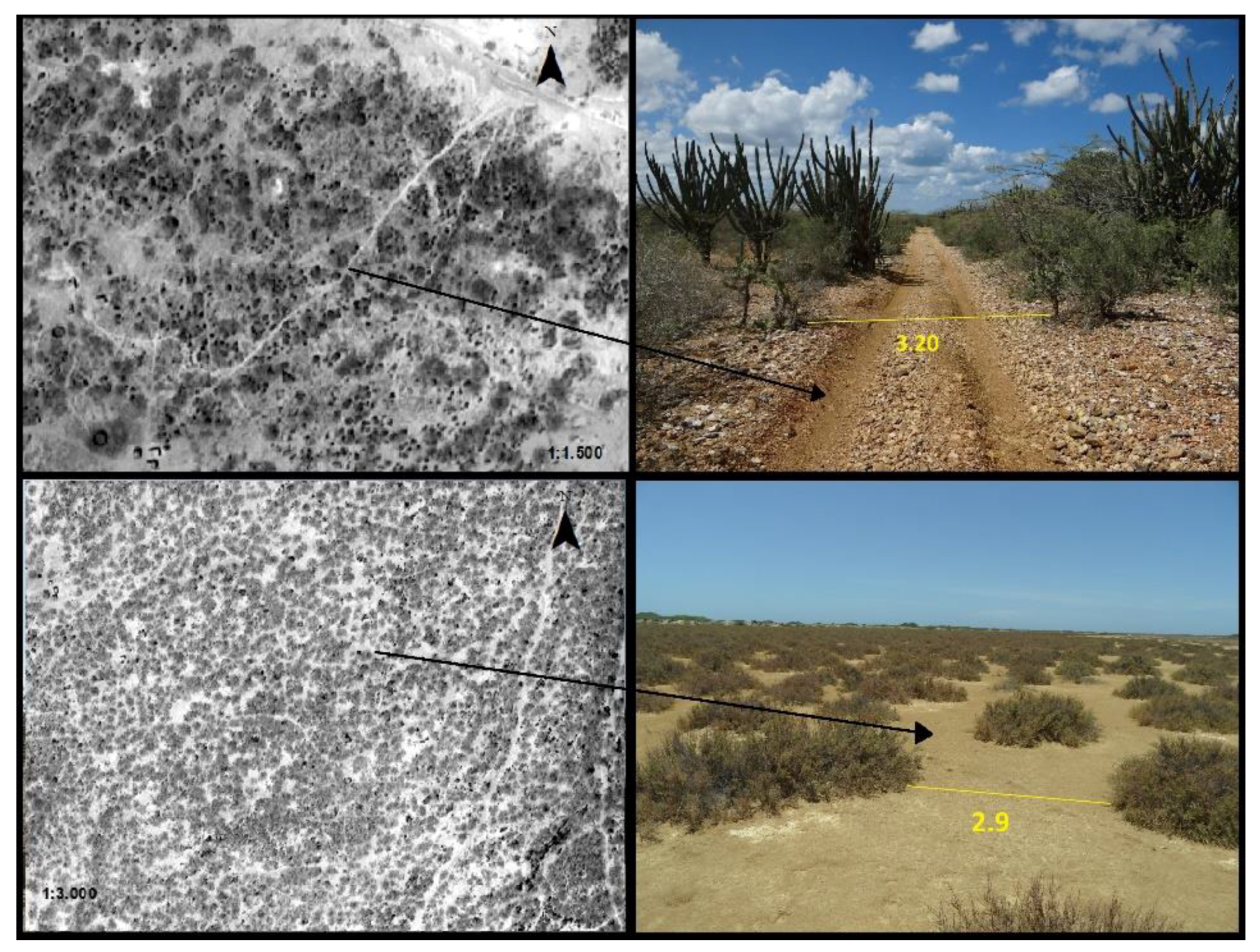
3.4. Measurement of Distances between Patches, Fragmentation
The distances between vegetation in dry areas is a very important factor in how the leopard pattern behaves in an area like La Guajira. A number of measurements were made in the field to be used as a reference when defining the distances between the patches of vegetation (Figure 10).
FRAGSTATS is a spatial pattern analysis program for quantifying landscape structure (Table 6). The landscape subject to analysis is user-defined and can represent any spatial phenomenon. It quantifies the areal extent and spatial distribution of patches (i.e., polygons on a map coverage) within a landscape; it is incumbent upon the user to establish a sound basis for defining and scaling the landscape (including the extent and grain of the landscape) and the scheme upon which patches within the landscape are classified and delineated [52].
FRAGSTATS software, part of the ArcGris programme, was used to study this behaviour, and analyze how vegetation cover has fragmented over the years (1965, 2007 and 2013). Once the coverage information for the 3 years was established, the indices were determined. Firstly, the total extension of coverage (CA) was calculated in m2, and then divided by 10,000 to give a total in hectares. The next stage was the calculation of the number of patches (NP), providing an indication of the degree of fragmentation, particularly if the habitat or land use in the area was originally relatively homogenous. The larger the number of fragments, the greater the influence it will have on the landscape’s fragmentation. Finally, the average index of the Euclidian distance (ENN_MN) was calculated. This measurement is the total of the distance between one patch and the closest patch of the same type, based on the distance between edges, divided by the number of patches of the same type [53]. This index indicates the degree of isolation between fragments of the same type. In the study area, the dominant coverage according to the total area (CA) was mostly bare soil (Table 7).
The Number of Patches (NP) was calculated for each class, which indicates the degree of fragmentation, especially if in its initial state the region was relatively homogeneous in terms of type of habitat or land use. The greater the number of fragments, the greater the influence on the fragmentation of the landscape (Table 8).
This is evidence that bare soil tends to be compacted into ever larger fragments, and tree classes into ever smaller fragments, as can be seen in the average patch size index AREA_MN (Table 9).
Analyzing the NP and AREA_MN indices together shows that the fragmentation of the area increased. Finally, the average value of the distance between one fragment and another can be seen using the ENN_MN index. For the tree class, the average distance between patches was 8 m in 1965, 4 m in 2007 and 3 m in 2013; these results coincide with the measurements made on the ground in 2014. Bare soil changed from an average of 7 m in 1965 to 4 m in 2007, a figure that remained the same in 2013. The distance between low vegetation was 15 m in 1965, falling to 6 m in the following years.
4. Discussion and Conclusions
The results can clearly be extrapolated to other places if we bear in mind that Fuentes et al. [32] managed to demonstrate that the Leopard pattern presents itself in a wide variety of places around the world, mainly because they share very similar environmental conditions. Grazing pressure from ungulates was a result that was mentioned in the literature [5,54,55,56,57]. Heavy grazing and trampling by livestock in semi-arid regions, concentrated around water sources, often leads to a reduction in vegetation cover and soil compaction. This result is similarly mentioned in other studies. Excessive grazing can alter in situ plant-soil relationships and create spatial heterogeneity; References [58,59,60] suggested that vegetation patterns in semi-arid grasslands were created by herbivores’ selective grazing. Studies of the Tiger pattern in Australia mention its relationship with the pattern formation with bands of vegetation. Bands evolve as the dense vegetation cover thins due to climate deterioration or grazing pressure [61]. The extensive elimination of vegetation has been observed in western New South Wales (Australia) during dry years due to combined pressure from actions by rabbits and goats. Following stabilization of the model, the grazing pressure was eliminated and trends in the recovery of the Strip were observed [62]. These studies note that grazing and anthropogenic activities can modify vegetation patterns. One of the results consistent with those identified by other authors is the greater humidity in the areas where the vegetation is present. The resulting spatial variation can be structured on certain scales where patch vegetation concentrates nutrients and water in the soil, but these are eliminated in patches of bare or compacted soil [5,59,63,64,65,66,67,68].
Aguiar [5] specifies something that was partially corroborated in La Guajira. The basic mechanism is a redistribution of water, nutrients and seeds (resulting from the presence of dominant woody plants), which creates and maintains dense vegetation patches. Water is the major agent of redistribution in tiger vegetation, whereas wind and animals are the major cause of redistribution in leopard vegetation. Moreover, in tiger patterns, water is the main driver of secondary seed dispersal, whereas in leopard patterns, wind or animals are the main agents of dispersal [5]. The fragmentation of ecosystems, particularly in dry lands, is indicative of the reduction of ground cover and the accelerating pace of land degradation. Assessing the change in vegetation cover (leopard pattern) in the studied area shows that, over time, vegetation cover has fallen (18.72%), while there has been a rise in the extent of bare ground (81%). The lack of nutrients in the soil, along with low or inexistent rainfall, mean that vegetation cover is generally low in arid areas. However, large-scale vegetation fragmentation does not occur naturally, it requires an element that produces such a change in the natural balance of the area. This element is man and animals. The effect of man is clear in the whole area, and the satellite images show this effect on ground cover.
The fragmentation indices show the continuous reduction in ground cover, the increase in the number of shrub fragments, and the reduction in the size of vegetation patches. The opposite effect was observed on bare land, with fewer fragments, greater distances between them and an increase in the size of patches. Vegetation eco-system fragmentation is linked to anthropogenic pressure in the area; this is seen over time through the increase in the number of ranches, paths, jagüeyes and paddocks. This is evidence of the great pressure that vegetation and the area as a whole are subjected to year after year. Coverage was mainly affected by the breaking up of vegetation to create roads and paths for people, bicycles, motorbikes and 4 × 4 s. This change is shown in the combined map of all 3 years (1965, 2007 and 2013), providing evidence of the large number of roads and paths that exist in the study area (324.5 km in 2013), where they are evenly distributed across the entire area except on higher land, where there are very few. The other element that is linked to animals and plays a role in the fragmentation process is the effect of trampling on the ground. Animal hooves compact the soil and disrupt the natural balance. This compacting leads to the loss of nutrients, greatly reducing the amount of nitrogen and carbon provided due to the slower decomposition of the soil caused by the reduction in biota (bacteria and micro-organisms). It also becomes more impermeable, thus reducing the supply of water to plants through infiltration. Hardened or compacted layers cause a mechanical impediment that means that roots cannot penetrate the soil. This effect is more pronounced and faster on the paths built by people; with human footprints and vehicle tyres all compacting the soil.
Finally, the pattern derives from the fact that during the rainy season, the seeds (grasses and woody plants) trapped in the fertility island germinate due to the increase of humidity in the sand, and the improved local conditions facilitating its development. Within the fertility islands, the conditions are more favorable than those of the surrounding bare soils because there is greater infiltration in the islands due to the presence of plants. Water erosion redistributes the surface material during the rainy season, while during the dry season compacted soils and spaces fragmented by human and animal activity that contain sandy sediments are eliminated by the wind, leaving bare soil between patches of vegetation and thus forming the Leopard pattern.
Author Contributions
Conceptualization, J.F., D.V. and J.P.; Methodology, J.F.; Software, J.F.; Validation, J.F., D.V. and J.P.; Formal Analysis, J.F.; Investigation, J.F.; Resources, J.F., D.V. and J.P.; Data Curation, J.F.; Writing-Original Draft Preparation, J.F., D.V. and J.P.; Writing-Review & Editing, J.F., D.V. and J.P.
Funding
This research was supported by the PhD scholarship COLCIENCIAS, Colombia (exterior 568).
Conflicts of Interest
The authors declare no conflict of interest.
References
- Millennium Ecosystem Assessment Board. Ecosystems and Human Well-Being: Desertification Synthesis; World Resources Institute: Washington, DC, USA, 2005. [Google Scholar]
- Colombia. Ministerio del Medio Ambiente. Poltica Nacional Ambiental Para el Desarrollo Sostenible de Los Espacios Oceǹicos y Las Zonas Costeras e Insulares de Colombia; Ministerio del Medio Ambiente: Bogotá, Colombia, 2001.
- Rojas, M.Y.; Alonso, L.A.; Sarmiento, V.A.; Eljach, L.Y.; Usaquén, W. Structure analysis of the la Guajira-Colombia population: A genetic, demographic and genealogical overview. Ann. Hum. Biol. 2013, 40, 119–131. [Google Scholar] [CrossRef] [PubMed]
- Colombia. Ministerio de Ambiente, Vivienda y Desarrollo Territorial, and Instituto de Hidrologia, Meteorologia y Estudios Ambientales (IDEAM). Atlas climático de Colombia; Instituto de Hidrología, Meteorología y Estudios Ambientales: Bogotá, Colombia, 2005.
- Aguiar, M.; Sala, O.E. Patch structure, dynamics and implications for the functioning of arid ecosystems. Trends Ecol. Evol. 1999, 14, 273–277. [Google Scholar] [CrossRef]
- Rietkerk, M.; van de Koppel, J. Regular pattern formation in real ecosystems. Trends Ecol. Evol. 2008, 23, 169–175. [Google Scholar] [CrossRef] [PubMed]
- Cheng, Y.; Stieglitz, M.; Engel, V.; Turk, G. Parallel vegetation stripe formation through hydrologic interactions. In EGU General Assembly Conference Abstracts, Proceedings of the European Geophysical Union Conference, Vienna, Austria, 2–7 May 2010; EGU: Munich, Germany, 2010; Volume 12, p. 7498. [Google Scholar]
- Meigs, P. World distribution of arid and semi-arid hot climates. In Reviews of Research on Arid Zone Hydrology; UNESCO: Paris, France, 1953. [Google Scholar]
- Slatyer, R.O. Methodology of a water balance study conducted on a desert woodland (acacia aneura f. Muell.) community in central Australia. In Symposium on Plant-Water Relationships in Arid and Semi-Arid Conditions; UNESCO, Ed.; UNESCO document: Madrid, Spain, 1959; p. 13. [Google Scholar]
- Warren, A. Some vegetation patterns in the republic of the sudan—A discussion. Geoderma 1973, 9, 75–78. [Google Scholar] [CrossRef]
- Worrall, G. The butana grass patterns. J. Soil Sci. 1959, 10, 34–53. [Google Scholar] [CrossRef]
- Lejeune, O.; Tlidi, M.; Couteron, P. Localized vegetation patches: A self-organized response to resource scarcity. Phys. Rev. E 2002, 66, 010901. [Google Scholar] [CrossRef] [PubMed]
- Tlidi, M.; Lefever, R.; Vladimirov, A. On vegetation clustering, localized bare soil spots and fairy circles. In Dissipative Solitons: From Optics to Biology and Medicine; Springer: Berlin/Heidelberg, Germany, 2008; pp. 1–22. [Google Scholar]
- Escaff, D.; Fernandez-Oto, C.; Clerc, M.G.; Tlidi, M. Localized vegetation patterns, fairy circles, and localized patches in arid landscapes. Phys. Rev. E 2015, 91, 022924. [Google Scholar] [CrossRef] [PubMed]
- Couteron, P.; Anthelme, F.; Clerc, M.; Escaff, D.; Fernandez-Oto, C.; Tlidi, M. Plant clonal morphologies and spatial patterns as self-organized responses to resource-limited environments. Phil. Trans. R. Soc. A. 2014, 372, 20140102. [Google Scholar] [CrossRef] [PubMed]
- Lejeune, O.; Tlidi, M. A model for the explanation of vegetation stripes (tiger bush). J. Veg. Sci. 1999, 10, 201–208. [Google Scholar] [CrossRef]
- Bordeu, I.; Clerc, M.G.; Couteron, P.; Lefever, R.; Tlidi, M. Self-replication of localized vegetation patches in scarce environments. Sci. Rep. 2016, 6, 33703. [Google Scholar] [CrossRef] [PubMed]
- Tlidi, M.; Bordeu, I.; Clerc, M.G.; Escaff, D. Extended patchy ecosystems may increase their total biomass through self-replication. Ecol. Indic. 2018, 94, 534–543. [Google Scholar] [CrossRef] [Green Version]
- Borgogno, F.; D’Odorico, P.; Laio, F.; Ridolfi, L. Mathematical models of vegetation pattern formation in ecohydrology. Rev. Geophys. 2009, 47, RG1005. [Google Scholar] [CrossRef]
- Wickens, G.; Collier, F. Some vegetation patterns in the republic of the sudan. Geoderma 1971, 6, 43–59. [Google Scholar] [CrossRef]
- Soriano, A.; Sala, O.E.; Perelman, S.B. Patch structure and dynamics in a patagonian arid steppe. Vegetatio 1994, 111, 127–135. [Google Scholar] [CrossRef]
- Sala, O.E.; Aguiar, M.R. Origin, maintenance, and ecosystem effect of vegetation patches in arid lands. In Proceedings of the Vth International Rangeland Congress, Salt Lake City, UT, USA, 23–28 July 1995; pp. 29–32. [Google Scholar]
- Lefever, R.; Lejeune, O. On the origin of tiger bush. Bull. Math. Biol. 1997, 59, 263–294. [Google Scholar] [CrossRef]
- Leprun, J.C. The influences of ecological factors on tiger bush and dotted bush patterns along a gradient from mali to northern burkina faso. Catena 1999, 37, 25–44. [Google Scholar] [CrossRef]
- Couteron, P.; Lejeune, O. Periodic spotted patterns in semi-arid vegetation explained by a propagation-inhibition model. J. Ecol. 2001, 89, 616–628. [Google Scholar] [CrossRef]
- Meron, E.; Gilad, E.; von Hardenberg, J.; Shachak, M.; Zarmi, Y. Vegetation patterns along a rainfall gradient. Chaos Solitons Fractals 2004, 19, 367–376. [Google Scholar] [CrossRef] [Green Version]
- Imeson, A.; Prinsen, H. Vegetation patterns as biological indicators for identifying runoff and sediment source and sink areas for semi-arid landscapes in Spain. Agric. Ecosyst. Environ. 2004, 104, 333–342. [Google Scholar] [CrossRef]
- Bestelmeyer, B.T.; Ward, J.P.; Havstad, K.M. Soil-geomorphic heterogeneity governs patchy vegetation dynamics at an arid ecotone. Ecology 2006, 87, 963–973. [Google Scholar] [CrossRef]
- Bisigato, A.J.; Villagra, P.E.; Ares, J.O.; Rossi, B.E. Vegetation heterogeneity in monte desert ecosystems: A multi-scale approach linking patterns and processes. J. Arid Environ. 2009, 73, 182–191. [Google Scholar] [CrossRef]
- Yetemen, O.; Istanbulluoglu, E.; Vivoni, E.R. The implications of geology, soils, and vegetation on landscape morphology: Inferences from semi-arid basins with complex vegetation patterns in central New Mexico, USA. Geomorphology 2010, 116, 246–263. [Google Scholar] [CrossRef]
- Juergens, N.; Oldeland, J.; Hachfeld, B.; Erb, E.; Schultz, C. Ecology and spatial patterns of large-scale vegetation units within the central namib desert. J. Arid Environ. 2012, 93, 59–79. [Google Scholar] [CrossRef]
- Fuentes, J.; Varga, D.; Boada, M. Distribución del patrón espacial tipo leopardo en regiones áridas y semiáridas del mundo. Boletín de la Asociación de Geógrafos Españoles 2016, 71, 59–72. (In Spanish) [Google Scholar]
- MacDonald, R.A. Corona between the Sun & the Earth: The First Nro Reconnaissance Eye in Space; American Society for Photogrammetry and Remote Sensing: Bethesda, MD, USA, 1997. [Google Scholar]
- Galiatsatos, N. Assessment of the corona series of satellite imagery for landscape archaeology: A case study from the orontes valley, syria. Ph.D. Thesis, Durham University, Durham, UK, 2004. [Google Scholar]
- Challis, K.; Priestnall, G.; Gardner, A.; Henderson, J.; O’Hara, S. Corona remotely-sensed imagery in dryland archaeology: The islamic city of al-raqqa, syria. J. Field Archaeol. 2002, 29, 139–153. [Google Scholar] [CrossRef]
- Lovell, A.M.; Carr, J.R.; Stokes, C.R. Topographic controls on the surging behaviour of Sabche glacier, Nepal (1967 to 2017). Remote Sens. Environ. 2018, 210, 434–443. [Google Scholar] [CrossRef]
- Ni, N.; Chen, N.; Ernst, R.E.; Yang, S.; Chen, J. Semi-automatic extraction and mapping of dyke swarms based on multi-resolution remote sensing images: Applied to the dykes in the kuluketage region in the northeastern tarim block. Precambrian Res. 2018. [Google Scholar] [CrossRef]
- Janssen, T.A.J.; Ametsitsi, G.K.D.; Collins, M.; Adu-Bredu, S.; Oliveras, I.; Mitchard, E.T.A.; Veenendaal, E.M. Extending the baseline of tropical dry forest loss in ghana (1984–2015) reveals drivers of major deforestation inside a protected area. Biol. Conserv. 2018, 218, 163–172. [Google Scholar] [CrossRef]
- Saleem, A.; Corner, R.; Awange, J. On the possibility of using corona and landsat data for evaluating and mapping long-term lulc: Case study of iraqi kurdistan. Appl. Geogr. 2018, 90, 145–154. [Google Scholar] [CrossRef]
- Nita, M.D.; Munteanu, C.; Gutman, G.; Abrudan, I.V.; Radeloff, V.C. Widespread forest cutting in the aftermath of world war ii captured by broad-scale historical corona spy satellite photography. Remote Sens. Environ. 2018, 204, 322–332. [Google Scholar] [CrossRef]
- Watanabe, N.; Nakamura, S.; Liu, B.; Wang, N. Utilization of structure from motion for processing corona satellite images: Application to mapping and interpretation of archaeological features in Liangzhu culture, China. Archaeol. Res. Asia 2017, 11, 38–50. [Google Scholar] [CrossRef]
- Mihai, B.; Nistor, C.; Toma, L.; Săvulescu, I. High resolution landscape change analysis with corona kh-4b imagery. A case study from iron gates reservoir area. Procedia Environ. Sci. 2016, 32, 200–210. [Google Scholar] [CrossRef]
- Scollar, I.; Galiatsatos, N.; Mugnier, C. Mapping from corona: Geometric distortion in kh4 images. Photogramm. Eng. Remote Sens. 2016, 82, 7–13. [Google Scholar] [CrossRef]
- Song, D.-X.; Huang, C.; Sexton, J.O.; Channan, S.; Feng, M.; Townshend, J.R. Use of landsat and corona data for mapping forest cover change from the mid-1960s to 2000s: Case studies from the eastern united states and central brazil. ISPRS J. Photogramm. Remote Sens. 2015, 103, 81–92. [Google Scholar] [CrossRef]
- Hritz, C. A malarial-ridden swamp: Using google earth pro and corona to access the southern balikh valley, syria. J. Archaeol. Sci. 2013, 40, 1975–1987. [Google Scholar] [CrossRef]
- Federal Geographic Data Committee. Geospatial Positioning Accuracy Standards, Part 3: National Standard for Spatial Data Accuracy. In Subcommittee for Base Cartographic Data; Federal Geographic Data Committee: Reston, VA, USA, 1998; p. 25. [Google Scholar]
- Research Systems Inc. Envi User’s Guide. Available online: http://aviris.gl.fcen.uba.ar/Curso_SR/biblio_sr/ENVI_userguid.pdf (accessed on 20 September 2018).
- Carletta, J. Assessing agreement on classification tasks: The kappa statistic. Comput. Linguist. 1996, 22, 249–254. [Google Scholar]
- Chuvieco, E.; Salas, J. Mapping the spatial distribution of forest fire danger using gis. Int. J. Geogr. Inf. Sci. 1996, 10, 333–345. [Google Scholar] [CrossRef]
- Congalton, R.G. A review of assessing the accuracy of classifications of remotely sensed data. Remote Sens. Environ. 1991, 37, 35–46. [Google Scholar] [CrossRef]
- Arnold, G.; Arnold, M.; Dudzinsky, M. Ethology of Free-Ranging Domestic Animals; Elsevier Scientific Publishing Co.: Amsterdam, NY, USA, 1978; p. 210. [Google Scholar]
- McGarigal, K.; Marks, B.J. Spatial pattern analysis program for quantifying landscape structure. Dolores (CO) PO Box 1994, 606, 67. [Google Scholar]
- McGarigal, K.; Cushman, S.A. Comparative evaluation of experimental approaches to the study of habitat fragmentation effects. Ecol. Appl. 2002, 12, 335–345. [Google Scholar] [CrossRef]
- Elwell, H.; Stocking, M. Vegetal cover to estimate soil erosion hazard in Rhodesia. Geoderma 1976, 15, 61–70. [Google Scholar] [CrossRef]
- Kelly, R.; Walker, B. The effects of different forms of land use on the ecology of a semi-arid region in south-eastern Rhodesia. J. Ecol. 1976, 64, 553–576. [Google Scholar] [CrossRef]
- Breman, H.; De Wit, C. Rangeland productivity and exploitation in the Sahel. Science 1983, 221, 1341–1347. [Google Scholar] [CrossRef] [PubMed]
- Stroosnijder, L. Modelling the effect of grazing on infiltration, runoff and primary production in the Sahel. Ecol. Model. 1996, 92, 79–88. [Google Scholar] [CrossRef]
- Schlesinger, W.H.; Reynolds, J.F.; Cunningham, G.L.; Huenneke, L.; Jarrell, W.; Virginia, R.; Whitford, W. Biological feedbacks in global desertification. Science 1990, 247, 1043–1048. [Google Scholar] [CrossRef] [PubMed]
- Schlesinger, W.H.; Pilmanis, A.M. Plant-soil interactions in deserts. Biogeochemistry 1998, 42, 169–187. [Google Scholar] [CrossRef]
- Kellner, K.; Bosch, O. Influence of patch formation in determining the stocking rate for southern African grasslands. J. Arid Environ. 1992, 22, 99–105. [Google Scholar]
- Dunkerley, D.; Brown, K. Runoff and runon areas in a patterned chenopod Shrubland, arid western New South Wales, Australia: Characteristics and origin. J. arid Environ. 1995, 30, 41–55. [Google Scholar] [CrossRef]
- Dunkerley, D. Banded vegetation: Survival under drought and grazing pressure based on a simple cellular automaton model. J. Arid Environ. 1997, 35, 419–428. [Google Scholar] [CrossRef]
- Tongway, D.J.; Ludwig, J.A. Vegetation and soil patterning in semi-arid Mulga lands of Eastern Australia. Austral Ecol. 1990, 15, 23–34. [Google Scholar] [CrossRef]
- Valentin, C.; d’Herbès, J.M. Niger tiger bush as a natural water harvesting system. Catena 1999, 37, 231–256. [Google Scholar] [CrossRef]
- Wilson, J.P.; Gallant, J.C. Terrain Analysis: Principles and Applications; John Wiley & Sons: Hoboken, NJ, USA, 2000. [Google Scholar]
- Menaut, J.C.; Walker, B.; Tongway, D.J.; Valentin, C.; Seghieri, J. Banded Vegetation Patterning in Arid and Semiarid Environments: Ecological Processes and Consequences for Management; Springer Science & Business Media: Berlin, Germany, 2001; Volume 149. [Google Scholar]
- Ursino, N. The influence of soil properties on the formation of unstable vegetation patterns on hillsides of semiarid catchments. Adv. Water Resour. 2005, 28, 956–963. [Google Scholar] [CrossRef]
- Saco, P.; Willgoose, G.; Hancock, G. Eco-geomorphology of banded vegetation patterns in arid and semi-arid regions. Hydrol. Earth Syst. Sci. 2007, 11, 1717–1730. [Google Scholar] [CrossRef] [Green Version]
Figure 1.
Tiger bush pattern (A), Somalia 2010 (7°46’51.15” N, 47°55’38.56” E); and leopard bush pattern (B), La Guajira 2007 (12°8’6.54” N, 72°7’25.92” W). QuickBird—ArcGIS Online data.
Figure 1.
Tiger bush pattern (A), Somalia 2010 (7°46’51.15” N, 47°55’38.56” E); and leopard bush pattern (B), La Guajira 2007 (12°8’6.54” N, 72°7’25.92” W). QuickBird—ArcGIS Online data.

Figure 2.
Location of study area, Cabo de la Vela, La Guajira.

Figure 3.
Stereoscopic images (A, above; B, below) from the Corona KH-4A satellite, 6 October 1965 of Cabo de la Vela.
Figure 3.
Stereoscopic images (A, above; B, below) from the Corona KH-4A satellite, 6 October 1965 of Cabo de la Vela.

Figure 4.
QuickBird image 15 March 2007 of Cabo de la Vela.

Figure 5.
Eros B stereoscopic images (A MBT1-e2376518, left; B MBT1-e2376519, right 6 February 2013).
Figure 5.
Eros B stereoscopic images (A MBT1-e2376518, left; B MBT1-e2376519, right 6 February 2013).

Figure 6.
DTM resulting from the extraction of the DSM from the Eros B Images A, flat area; B, Mountain range.
Figure 6.
DTM resulting from the extraction of the DSM from the Eros B Images A, flat area; B, Mountain range.

Figure 7.
Land use and cover 1965.

Figure 8.
Land use and cover 1997.

Figure 9.
Land use and cover 2013.

Figure 10.
Distance measurements between leopard patches on the ground and the satellite image Eros B.
Figure 10.
Distance measurements between leopard patches on the ground and the satellite image Eros B.


Table 1.
Presence of the Leopard pattern in bibliographic references.
| Place | Continent | Distance | References |
|---|---|---|---|
| Sudan | Africa | 30–50 m | 1971 [20] |
| Argentina | America | 2 m | 1994 [21] |
| Argentina | America | 2 m | 1996 [22] |
| Nigeria | Africa | 2–50 m | 1997 [23] |
| Burkina Faso y Mali | Africa | 60–180 m | 1999 [24] |
| Mayo River—Argentina | America | 2 m | 1999 [5] |
| Burkina Faso | Africa | 30–50 m | 2001 [25] |
| Negev—Israel | Asia | 1–2 m | 2004 [26] |
| Spain | Europe | 1–2 m | 2004 [27] |
| Chihuahua Las Cruces, NM | America | 1–2 m | 2006 [28] |
| Zambia | Africa | 15–30 m | 2009 [19] |
| Del Monte Desert, Argentina | America | 2–3 m | 2009 [29] |
| New Mexico | America | 20–40 m | 2010 [30] |
| Namibia | Africa | 3–5 m | 2012 [31] |
Table 2.
Studies that use Corona images.
| Place | Field of Study | References |
|---|---|---|
| Sabche Glacier, Nepal | Topographic control | 2018 [36] |
| Tarim Block, northwestern China | Mapping of mafic dykes | 2018 [37] |
| Kogyae Strict Nature Reserve, Ghana | Deforestation | 2018 [38] |
| Iraqi Kurdistan, Iraq | Land use change | 2018 [39] |
| Carpathian Mountains, Romania | Land use change | 2018 [40] |
| Shanghai, China | Archaeological | 2017 [41] |
| Danube River, Romania and Serbia. | Landscape | 2016 [42] |
| EE.UU. | Mapping | 2016 [43] |
| EE.UU. and Brazil | Land use change | 2016 [44] |
| Balikh River valley, Syria. | Archaeological | 2013 [45] |
Table 3.
Resulting error values in EROS B images.
| Point | Residual | X: RMS | Y: RMS |
|---|---|---|---|
| MBT1-E2376518 | 0.78 | 1.64 | 0.83 |
| MBT1-E2376519 | 0.99 | 1.90 | 0.91 |
| Tie points | 0.26 | 0.71 | 0.45 |
| Check points | 0.17 | 0.83 | 0.66 |
Table 4.
Maximum expected error according to scale variation FGDC [46].
Table 4.
Maximum expected error according to scale variation FGDC [46].
| Scale | RMSE (m) |
|---|---|
| 1:50 | 0.0125 |
| 1:100 | 0.025 |
| 1:200 | 0.050 |
| 1:500 | 0.125 |
| 1:1000 | 0.25 |
| 1:2000 | 0.50 |
| 1:4000 | 1.00 |
| 1:5000 | 1.25 |
| 1:10,000 | 2.50 |
| 1:20,000 | 5.00 |
Table 5.
Classes used to classify vegetation cover and land use.
| Cover | Description | Use | Description |
|---|---|---|---|
| Bare soil | Refers to soil that does not have a continuous surface layer that protects it from weather; this means that it is damaged by water or wind. | Paths | All visible paths produced by vehicles, people and animals. |
| Tree | Group of mainly tree and cacti species that form plant associations. | Paddock | The place where animals are kept (mostly ungulates) |
| Low vegetation | Low vegetation coverage in sandy soils of the coastal area produced by plant associations. | Ranches | A group of ranches or cabins that make up a settlement inhabited by the indigenous Wayúu community. |
| Jaguey | A Colombian term referring to a body of artificial surface water for human and animal use. |
Table 6.
Indices used of FRAGSTATS.
| Index | Description | Formula |
|---|---|---|
| Class area (CA) | CA equals the sum of the areas (m²) of all patches of the corresponding patch type, divided by 10,000 (to convert to hectares); that is, total class area. | |
| Number of Patches (NP) | NP equals the number of patches of the corresponding patch type (class). | |
| Euclidean Nearest Neighbor Distance (ENM_MN) | MN (Mean) equals the sum, across all patches in the landscape, of the corresponding patch metric values, divided by the total number of patches. MN is given in the same units as the corresponding patch metric. | |
| Mean patch area (AREA_MN) |
Table 7.
Total area of coverage (CA) for the different years.
| Cover | 2013 | 2007 | 1965 | ||||
|---|---|---|---|---|---|---|---|
| ha | % | ha | % | ha | % | ||
| Bare soil | 3.495 | 81.29 | 3.595 | 83.62 | 3.366 | 78.29 | |
| Tree | 800 | 18.6 | 692 | 16.07 | 924 | 21.49 | |
| Low vegetation | 4 | 0.1 | 12 | 0.28 | 9 | 0.22 | |
| Total | 4.299 | 100 | 4.299 | 100 | 4.299 | 100 | |
Table 8.
Number of patches (NP) for the different years.
| Cover | 2013 | 2007 | 1965 |
|---|---|---|---|
| Number of patches | Number of patches | Number of patches | |
| Bare soil | 2.168 | 2.610 | 4.314 |
| Tree | 136.328 | 168.240 | 25.803 |
| Low vegetation | 1.249 | 1.347 | 446 |
| Total | 139.745 | 172.197 | 30.563 |
Table 9.
Mean patch area (AREA_MN) for the different years.
| Cover | 2013 | 2007 | 1965 |
|---|---|---|---|
| m² | m² | m² | |
| Bare soil | 15.200 | 13.704 | 7.811 |
| Tree | 73 | 41 | 358 |
| Low vegetation | 37 | 91 | 203 |
© 2018 by the authors. Licensee MDPI, Basel, Switzerland. This article is an open access article distributed under the terms and conditions of the Creative Commons Attribution (CC BY) license (http://creativecommons.org/licenses/by/4.0/).
Share and Cite
MDPI and ACS Style
Fuentes, J.; Varga, D.; Pintó, J. The Use of High-Resolution Historical Images to Analyse the Leopard Pattern in the Arid Area of La Alta Guajira, Colombia. Geosciences 2018, 8, 366. https://doi.org/10.3390/geosciences8100366
AMA Style
Fuentes J, Varga D, Pintó J. The Use of High-Resolution Historical Images to Analyse the Leopard Pattern in the Arid Area of La Alta Guajira, Colombia. Geosciences. 2018; 8(10):366. https://doi.org/10.3390/geosciences8100366
Chicago/Turabian StyleFuentes, José, Diego Varga, and Josep Pintó. 2018. "The Use of High-Resolution Historical Images to Analyse the Leopard Pattern in the Arid Area of La Alta Guajira, Colombia" Geosciences 8, no. 10: 366. https://doi.org/10.3390/geosciences8100366
Note that from the first issue of 2016, this journal uses article numbers instead of page numbers. See further details here.