Assessment of Leachate Production from a Municipal Solid-Waste Landfill through Water-Balance Modeling

Abstract

Mineral temporary capping systems of landfills are required to accomplish the long-term coverage prerequisites or to use them as a basis layer prior to later permanent sealing. Such a capping system for a municipal waste landfill in Rastorf (Northern Germany) was developed and tested for its sealing capability on the basis of observed and simulated water balance components for the period between 2008 and 2015, considering observed local weather data and complemented by the Hydraulic Evaluation of Landfill Performance (HELP 3.95 D) model. The modeling results of this case study could be improved by the correction of previously used global solar radiation data due to the consideration of exposure and inclination angle of landfill surface areas. The model could positively be validated by comparing observed and simulated outflow (surface runoff and lateral drainage) data with R² values ranging between 0.95 and 0.99, as well as for the leachate rates with R² values of 0.78–0.87. The statistical-empirical HELP model was found useful in predicting the leachate generation of a temporary landfill capping system for specific soil and site conditions, even if only a restricted set of observed data was available.

1. Introduction

Landfill capping systems as engineered barriers are purposed to prevent or minimize the contact of precipitation or melting water percolation with the waste body to limit the generation of leachate or gas emissions, which may reach the aquifer system or the atmosphere, respectively [1,2,3].

A landfill requires a combination of a top capping and a bottom liner, often constructed of natural materials with appropriate hydraulic conductivity, complemented by geosynthetics and geotextiles [4]. An appropriate choice of vegetation is equally important to establish a protective vegetation cover to improve the soil physical properties, the soil anti-erodibility, and the reduction of runoff and erosion [5,6].

Therefore, semipermeable temporary capping systems (i.e., Rastorf landfill) enable a specific ‘shutdown’ of the bioreactor by a controlled infiltration of precipitation water into the waste body (2.0 × 10⁹ kg of municipal waste) and also allow biogas extraction during phases of waste-body settlement [7]. After the consolidation of the waste body, the temporary cover can be replaced by a long-term sealing system that meets statutory requirements [8]. In order to lower these additional financial costs, it is also possible and advisable to include the well-functioning temporary capping system layers in the final one, which may even increase or maintain long-term impermeability.

The effectiveness of a capping system can be assessed by the water balance or leachate generation under the specific climate and soil conditions [9]. There are several modeling approaches of landfill capping systems, with and without geosynthetics and geotextiles, combining water balance calculations with the predominant statistical-empirical Hydraulic Evaluation of Landfill Performance (HELP) model [10,11,12], numerical models of soil water flow and solute transport such as in the HYDRUS program, or the Finite Element subsurface FLOW system program (FEFLOW) [13,14,15]. Such predictive models can be used to support the planning of a landfill, to optimize the particular system from an economic point of view [3], and to verify the long-term hydraulic stability of a final capping system.

This study presents a practical example to show that the HELP model is useful to solve scientific issues with regard to the water balance of landfill capping systems. It is also a scientific fundament for other young professionals considering the very limited amount of scientific writings including simulations of the HELP 3.95 D model. As a novelty, surface area factor v was implemented in the model routine on the basis of global solar radiation. Moreover, anisotropic water-flow conditions of the Rastorf landfill were modeled through modifying the standard construction of the landfill with a drainage layer instead of a vertical percolation layer.

This study includes the observed and modeled water-balance data of the Rastorf landfill, collected between 2008 and 2015. These data are compared with the results simulated with the HELP 3.95 D model.

The authors hypothesize that (a) relatively realistic modeling results can already be obtained with a limited set of observed data and (b) the spatial heterogeneity of global solar radiation at three differently exposed and inclined landfill areas strongly affects modeling results.

Furthermore, this paper discusses the applicability of a statistical-empirical model for predicting the leachate generation of landfill capping systems for the given site conditions.

2. Materials and Methods

2.1. Study Site

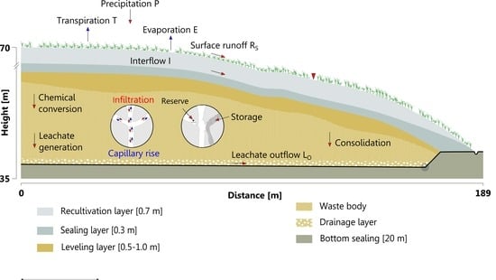
The Rastorf landfill in Schleswig-Holstein (Northern Germany) is divided into three areas: I (21,275 m²), II (29,961 m²), and III (22,208 m²), and consists of a bottom layer of hardly permeable clay up to 20 m thick (Figure 1).

A high-density polyethylene layer of 2.5 mm thickness and an added drainage system above the clayey bottom layer collects the leachate before treatment by reverse osmosis.

The 1.0 m thick mineral capping system consists of a recultivation layer and a sealing layer. The recultivation layer consists of a 0.4 m humic top soil and a 0.3 m sandy loam substrate with minor organic carbon content in its function as combined evapotranspiration and lateral drainage layer above the sealing layer. The 0.3 m thick sealing layer serves as root barrier and provides a downslope lateral drainage (interflow) below the recultivation layer.

The landfill surface is covered with different types of grass: Perennial ryegrass (Lolium perenne), meadow fescue (Festuca pratensis), red fescue (Festuca rubra), sheep fescue (Festuca ovina), and orchard grass (Dactylis glomerata) with a surface distribution of 90%–95%, while the rest is distributed among white clover (Trifolium repens) and red clover (Trifolium pratense). In relation to grassland management, two cuts per year are essential.

2.2. Laboratory Measurements

In 2015, more than 160 undisturbed soil cores (100 cm³) were sampled in the capping system in the vertical (90°) and horizontal (0°) directions in Area I (54°28′20″ N, 10°32′60″ E), II (54°28′11″ N, 10°32′71″ E), and III (54°28′08″ N, 10°32′75″ E) in depths of 0.2, 0.5, and 0.8 m, respectively, and then analyzed with different measurement devices. Saturated hydraulic conductivity (Ks in cm/s) was measured under dynamic conditions (10 soil cores per depth and direction) according to the procedure described by Reference [16]. Undisturbed soil cores (7 soil cores per depth and direction) were used to determine soil water retention characteristics with a combined pressure-plate method to determine the water content for 0, −6, and −30 kPa, and with a ceramic vacuum outflow method for −1500 kPa, as well as oven-dried at 105 °C, respectively [17].

2.3. Observation of the Water Balance Components of the Rastorf Landfill

In order to calculate the water balance for each area (I, II, III) a weather station (UGT, Freising, Germany) located close to the landfill (54°28′11″ N, 10°32′18″ E) recorded actual meteorological data, such as precipitation, air temperature, wind speed, wind direction, air pressure, and relative humidity, on daily basis. Global solar radiation was calculated on the basis of the following literature [18,19,20]. In addition, wind speed was measured at 10 m height and a logarithmic approximation was used to calculate wind speed for 2 m height [21]. Leaf area index (LAI) was calculated on the basis of the quarterly measured average vegetation height (z) in meters (m) in 8–10 repetitive transects (1 m²) per area with a folding ruler as follows [19]:

$$\mathrm{LAI}=24·\mathrm{z}$$

(1)

Actual evapotranspiration was estimated as a residual value using the water-balance equation; interception height was calculated according to the literature [22] with an LAI of 2 m²/m² in the winter period and 4 m²/m² in the summer period, respectively.

The surface runoff and the interflow were captured in 6 areas through (a) v-notch weirs with electric contact gauges that recorded water levels in the shafts and data loggers that calculate flow rates between 0.04 dm³/ and 315 dm³/s, and (b) tipping counters with a maximum flow capacity of 60 dm³ per 10 min, respectively. The leachate rate as water percolation through the waste body was estimated on a monthly basis using data from the landfill leachate-treatment (reverse osmosis) facility. In addition, changes in soil-moisture contents at the beginning of each year were continuously estimated by the Theta Probe ML2x frequency domain that recorded the water content in 0.2, 0.5, 0.8, and 1.0 m depth with a standard data logger DL 200 (Umwelt-Geräte-Technik GmbH, Müncheberg, Germany).

2.4. HELP Model

The HELP model is a quasi-two-dimensional hydrologic model that combines one-dimensional soil physical and hydrological processes in (a) vertical direction (saturated and unsaturated vertical flow) and (b) lateral direction (i.e., lateral drainage) according to the literature [10]. Thus, the model requires landfill design and weather data as well as material properties such as porosity (TP), field capacity (FC), wilting point (WP), and Ks values as input parameters, regularly [23]. In addition, the evaporative zone is typically equal to root depth, estimated with field-tracer experiments (Brilliant Blue tracer) and also calculated on the basis of FC, PWP, and actual water content for autumn in a dry year (i.e., 2008) following reference [24] that equals the maximum soil depth from which water can be removed through evapotranspiration [3,25]. With respect to the landfill design data, the upper part of the recultivation layer (0–0.4 m) was classified as the vertical percolation layer, the bottom part (0.4–0.7 m) was conducted as the lateral drainage layer to consider lateral saturated hydraulic conductivity, and the water flow between areas I, II, and III is restricted by the drainage system (constrained condition). The sealing layer was classified as the barrier soil liner.

Water balance calculations are based on analytical and empirical equations, of which a detailed description is given by the following equation [23,25],

$$\mathrm{L}\left({\mathrm{t}}_{\mathrm{i}}\right)=\mathrm{P}\left({\mathrm{t}}_{\mathrm{i}}\right)-\mathrm{ETa}\left({\mathrm{t}}_{\mathrm{i}}\right)-\mathrm{R}\left({\mathrm{t}}_{\mathrm{i}}\right)-\mathrm{D}\left({\mathrm{t}}_{\mathrm{i}}\right)\pm \Delta \mathrm{S}\left({\mathrm{t}}_{\mathrm{i}}\right)$$

(2)

where L = leachate rate, P = precipitation, ETa = actual evapotranspiration (including interception), R = runoff, D = lateral drainage, ∆S = change in soil moisture content in mm per year, and m³ and the time, t, is calculated in daily steps, subscript i, from 1 January 2012 until 31 December 2015 (1460 days).

The potential evapotranspiration consists of (a) evaporation of the surface water (primarily evaporation of intercepted water, plus the evaporation of snow), (b) soil evaporation, and (c) plant transpiration computed by a simplified approach [26],

$${\mathrm{E}}_{{\mathrm{o}}_{\mathrm{i}}}=\frac{{\mathrm{PENR}}_{\mathrm{i}}+{\mathrm{PENA}}_{\mathrm{i}}}{{\mathrm{L}}_{\mathrm{v}}}\mathrm{with}{\mathrm{L}}_{\mathrm{v}}=\{\begin{array}{c}59.7-0.0564{\mathrm{T}}_{{\mathrm{d}}_{\mathrm{i}}} \mathrm{for} \mathrm{water}\\ 67.67-0.0564{\mathrm{T}}_{{\mathrm{s}}_{\mathrm{i}}} \mathrm{for} \mathrm{snow}\end{array}$$

(3)

where E_oi = potential evapotranspiration on day i (mm), PENR_i = radiative component on day i (langleys), where 1 langley = 41,840 J/m², PENA_i = aerodynamic component on day i (langleys), L_v = latent heat for vaporization (for evaporating water) or latent heat of fusion (for evaporating snow) in langleys per mm of water, T_d = dew-point and T_s = snow temperature (°C).

The ETa was mainly calculated according to procedure described by reference [27] using a model of vegetation growth and decay [28]. Thus, the vegetative growth and decay submodel included in HELP was taken from the simulation model for water resources in rural basins (SWRRB) [28], whose developers adopted it in a simplified form from the EPIC model [29]. Therefore, FC (US: −33 kPa) is the lowest soil water content to allow unsaturated vertical flow (drainage) within the evaporative zone [30]. The interception-storage and interception-height capacity were calculated by the approach of reference [22], modified and adapted to German standards [31]. Vertical percolation (drainage) is modeled according to Darcy (1856) [32] using the equation for unsaturated hydraulic conductivity K(h) in cm/s, which again is based on the approach of reference [33]. Saturated lateral drainage is modeled after a steady-state solution of the Boussinesq equation in combination with the Dupuit–Forchheimer assumptions [34], which consider the Ks value of the drainage layer. The K(h) values for each soil layer were calculated based on measurements of changes in the water content and matric potential over depth and time as follows,

$$\mathrm{K}\left(\mathrm{h}\right)=\mathrm{Ks}{\left[\frac{\mathsf{\theta }-{\mathsf{\theta }}_{\mathrm{r}}}{\mathsf{\Phi }-{\mathsf{\theta }}_{\mathrm{r}}}\right]}^{3+\left(\frac{2}{\mathsf{\lambda }}\right)} \mathrm{with} {\mathsf{\theta }}_{\mathrm{r}}=\{\begin{array}{ll}0.6 \mathrm{WP}& \mathrm{WP}<0.04\\ 0.014+0.25 \mathrm{WP}& \mathrm{WP}\ge 0.04\end{array}$$

(4)

where θ = actual volumetric water content (m³/m³), θ_r = residual volumetric water content (m³/m³), Φ = total porosity (m³/m³), λ = pore-size distribution index (-), and WP = wilting point (m³/m³).

The HELP model allows only downward flow in barrier soil liners, while the leachate rate (percolation through the layer) depends upon the depth of the water-saturated soil (head) above the base of the layer, the liner thickness, and the Ks value of the barrier soil. Leachate occurs under those conditions whenever the moisture content of the layer above the liner is greater than the field capacity of the layer [23,25].

The rainfall–runoff process is modeled using the SCS curve-number method with values above 0 up to 100 [35]. Therefore, the curve number (CN) is an empirical parameter to predict runoff or infiltration from rainfall excess. CN values for areas I, II, and III were obtained under the terms of the surface slope, the slope length, and the vegetation cover, and also modified according to the previous sensitivity analysis [36],

$$\mathrm{R}=\{\begin{array}{ll}\frac{{\left(\mathrm{P}-{\mathrm{I}}_{\mathrm{a}}\right)}^2}{\mathrm{P}-{\mathrm{I}}_{\mathrm{a}}+\mathrm{S}}& \mathrm{P}>{\mathrm{I}}_{\mathrm{a}}\\ 0& \mathrm{P}\le {\mathrm{I}}_{\mathrm{a}}\end{array} \mathrm{with}\mathrm{S}=\frac{1000}{\mathrm{CN}}-10$$

(5)

where R = runoff (m³), P = precipitation (m³), S = potential maximum soil-moisture retention when the runoff begins (m³), I_a = initial water abstractions (sum of interception + evapotranspiration + infiltration + depression storage) in m³, and CN = curve number.

The lateral drainage layer required information about maximum drainage length as length of the horizontal projection of a representative flow path and the drain slope for areas I, II, and III. Therefore, the lateral drainage equation written in dimensionless form as [23],

$${\mathrm{y}}^{*}=\frac{{\mathrm{d}}^2{\mathrm{y}}^{*}}{{\mathrm{dx}}^{{*}^2}}+{\left(\frac{{\mathrm{dy}}^{*}}{{\mathrm{dx}}^{*}}\right)}^2+(\tan \mathsf{\alpha })\frac{{\mathrm{dy}}^{*}}{{\mathrm{dx}}^{*}}=\frac{{\mathrm{q}}_{\mathrm{D}}{}^{*}}{{\cos }^2\mathsf{\alpha }}$$

(6)

where x* = x/L (dimensionsless horizontal distance), y* = y/L (dimensionsless depth of saturation above liner), q_D* = q_D/K_D (dimensionsless lateral drainage rate) with K_D = saturated hydraulic conductivity of the drain layer (cm/s), and α = inclination angle of the liner surface.

2.5. Correction of Global Solar Radiation

Surface area factor v was implemented in the modeling approach and corresponds to the ratio of the monthly sums of global solar radiation (Rs) on inclined and horizontal reception areas considering the exposure and inclination angle (°) depending on a digital elevation model (grid width: 1 m) and a corrected albedo of 0.23 in the summer period (May 1 to October 31) and in the winter period (November 1 to April 30) following [20].

2.6. Model Calibration and Sensitivity Analysis

Calibration is the adaption of the model to reality; thus, various procedures are possible for calibration. In this study, the calibration procedure for the period from 2008 to 2011 is shown for Area I. Therefore, a so-called ‘zero alternative’ (za) was used, where all input variables were set to values determined in the laboratory. The ‘zero-alternative’ is not actually a calibration in the strict sense, but a simulation with observed values to check the quality of observed input quantities for the estimation of output quantities [37]. For calibration in the strict sense, input data were stepwise changed to minimize the deviation between the observed and modeled (a) outflow and (b) leachate data, also well described for the Rastorf landfill with the so-called ‘calibration alternative’ (ca) in the literature [38]. Analogous to the validation study for the HELP model [37], calibration data should be changed until the modeled output quantities are reproduced to within 0.1 mm of the observed data. The last step included the validation of the model for the period from 2012 to 2015, because the validity of the input and output data for the comparison of observed and modeled data is of major importance [31,39].

In this study, evaporative zone depth and slope gradient were used as parameters for sensitivity analysis, while soil physical properties did not change over time. Statistical quality criteria were used to represent the deviations between the modeled (x_mod) and the observed (x_obs) water balance parameters [40]. Therefore, the higher the arithmetic mean, the higher the root mean square error (RMSE):

$$\mathrm{RMSE}=\sqrt{\frac{1}{\mathrm{n}}{\displaystyle \sum }_{\mathrm{i}=1}^{\mathrm{n}}{\left({\mathrm{x}}_{\mathrm{mod}}-{\mathrm{x}}_{\mathrm{obs}}\right)}^2}$$

(7)

The RMSE observations’ standard deviation ratio (RSR) was calculated as the ratio of the RMSE and standard deviation of the observed data [41]:

$$\mathrm{RSR}=\frac{{{\displaystyle \sum }}_{\mathrm{i}=1}^{\mathrm{n}}\left({\mathrm{x}}_{\mathrm{obs}}-{\mathrm{x}}_{\mathrm{mod}}\right)·100}{{{\displaystyle \sum }}_{\mathrm{i}=1}^{\mathrm{n}}\left({\mathrm{x}}_{\mathrm{obs}}\right)}$$

(8)

The model quality can be obtained by the Nash–Sutcliffe efficiency index as the sum of the absolute squared differences between modeled and observed data as follows [39,42]:

$$\mathrm{NSE}=1-\frac{{{\displaystyle \sum }}_{\mathrm{i}=1}^{\mathrm{n}}{\left({\mathrm{x}}_{\mathrm{obs}}-{\mathrm{x}}_{\mathrm{mod}}\right)}^2}{{{\displaystyle \sum }}_{\mathrm{i}=1}^{\mathrm{n}}{\left({\mathrm{x}}_{\mathrm{obs}}-\overline{{\mathrm{x}}_{\mathrm{obs}}}\right)}^2}$$

(9)

In addition to a perfect linear relationship (NSE = 1), an NSE value < 0 indicates that the averaged observed data provide a better prediction of the problem than the modeled data [39].

The coefficient of determination (R²) is an index of goodness of fit and is determined from the covariance of the modeled and observed data and their individual variances [41]:

$${\mathrm{R}}^2={\left[\frac{{{\displaystyle \sum }}_{\mathrm{i}=1}^{\mathrm{n}}\left({\mathrm{x}}_{{\mathrm{mod}}_{\mathrm{i}}}-\overline{{\mathrm{x}}_{\mathrm{mod}}}\right)·\left({\mathrm{x}}_{{\mathrm{obs}}_{\mathrm{i}}}-\overline{{\mathrm{x}}_{\mathrm{obs}}}\right)}{\sqrt{{{\displaystyle \sum }}_{\mathrm{i}=1}^{\mathrm{n}}{\left({\mathrm{x}}_{{\mathrm{mod}}_{\mathrm{i}}}-\overline{{\mathrm{x}}_{\mathrm{mod}}}\right)}^2}·\sqrt{{{\displaystyle \sum }}_{\mathrm{i}=1}^{\mathrm{n}}{\left({\mathrm{x}}_{{\mathrm{obs}}_{\mathrm{i}}}-\overline{{\mathrm{x}}_{\mathrm{obs}}}\right)}^2}}\right]}^2$$

(10)

3. Results

3.1. Sensitivity Analysis

In a first step, sensitivity analysis was used to estimate the effects of changing input quantities. Therefore, an increasing evaporative zone depth from 0.2 m to 1.0 m increased the ETa from 325 up to 425 mm/year with regard to a constant LAI of 3.5 m²/m². An increasing LAI from 2 to 5 m²/m² enhanced the ETa from 330 to 410 mm/year considering a constant evaporative zone depth of 0.8 m. Additionally, a steeper slope of the drainage layer from 2% to 30% reduced the annual leachate rate of about 25% from 1.0 to 0.75 mm/year. The associated calibration study made it necessary to implement a lateral drainage layer instead of a vertical percolation layer in 0.4 to 0.7 m depth to consider the basic concept of the landfill capping system due to predominant Ks values of the compacted layer in the horizontal direction.

3.2. Model Calibration

The landfill design data and the soil physical properties (based on 2015 research, more clearly explained in Section 3.3) of the ‘zero-alternative’ (za) and the ‘calibration alternative’ (ca) of area I are described in

Table 1. Input data for calibration of the Hydraulic Evaluation of Landfill Performance (HELP) model. Landfill design and soil physical parameters. Data of area I with 7–10 undisturbed soil cores per layer for the average porosity values, field capacity (FC) at −33 kPa, wilting point (WP), and saturated hydraulic conductivity (Ks), including initial water content (WC) in 2008 and slope length and gradient.

Study Area and Layer		Porosity	FC	WP	Ks	WC	Slope Length and Gradient
		(m3/m3)	(m3/m3)	(m3/m3)	(m/s)	(m3/m3)	(m)/(%)
za	Percolation layer	0.356	0.184	0.127	4.5 × 107	0.212
	Drainage layer	0.317	0.206	0.136	5.6 × 106	0.244	44/28
	Barrier soil layer	0.292	0.175	0.121	3.7 × 107	0.194
ca	Percolation layer	0.356	0.184	0.127	4.5 × 106	0.212
	Drainage layer	0.317	0.206	0.136	5.6 × 104	0.244	72/12
	Barrier soil layer	0.292	0.175	0.121	3.7 × 109	0.194

. The Ks values of ca were increased for the percolation and drainage layer, and reduced for the barrier soil layer compared to za. The landfill design data (i.e., slope length) were not changed.

Between 2008 and 2011, evaporative zone depth was 0.5 m, annual vegetation periods ranged between 215 and 270 days, and the average maximum leaf area index was determined as 3.5 for a good stand of the grass [9], with a surface coverage of 100% (

Table 2. Input data for the HELP model: Evapotranspiration parameters (latitude 54.2°). Data of the weather station, including average wind speed and relative humidity, between 2008 and 2011.

Year	2008	2009	2010	2011
Average annual wind speed (m/s)	4.67	4.67	4.68	4.73
Average relative humidity (%)
1. Quarter (January 1 to March 31)	82.5	88.2	87.6	87.7
2. Quarter (April 1 to June 30)	70.6	71.2	77.5	73.8
3. Quarter (July 1 to September 30)	81.0	76.2	80.5	87.3
4. Quarter (October 1 to December 31)	91.1	89.4	93.1	93.9

).

Average annual wind speed varied between 4.67 m/s and 4.73 m/s, and average relative humidity between 70.6% and 93.9% (Table 2). The calculated LAI values were 3.0 m²/m² (November 1 to April 30), 3.4 m²/m² (May 1 to May 31), 4.1 m²/m² (June 1 to August 31), and 3.7 m²/m² (September 1 to October 31). The average surface area factor varied between 0.92 and 0.96 depending on the exposure and the slope gradient in

Table 3. Surface area factor v in the summer (May 1 to October 31) and winter period (November 1 to April 30), with the average slope gradient, slope length, and curve-number (SCS-CN method) of area I. The ± symbol corresponds to the standard deviation.

Area	I	II	III
Average slope gradient (°)	7 ± 3	14 ± 3	16 ± 4
Average slope length (m)	99 ± 65	48 ± 23	69 ± 4
Exposure	N/NE	SE	SW
Curve number (-)	72.9	74.7	75.5
Average value of v (-)
Summer period (May 1 to October 31)	0.92	1.13	1.15
Winter period (November 1 to April 30)	0.96	1.05	1.05

.

In the study period between 2008 and 2011, climatic water balance was positive (precipitation > evapotranspiration). The ETa was the most pronounced output value for ca and the observed data, while za was mostly intended by the leachate rate (

Table 4. Observed (obs) and modeled (za, ca) water-balance components of the temporary capping system for the zero alternative (za) and the calibration alternative (ca) between 2008 and 2011 in mm/year for area I. Precipitation is only observed. The ± symbol corresponds to standard deviation. The (–) symbol corresponds to irrational or missing data.

Water Balance (mm/year)	2008	2008	2008	2009	2009	2009	2010	2010	2010	2011	2011	2011
	za	ca	obs	za	ca	obs	za	ca	obs	za	ca	obs
Precipitation	689	689	689	726	726	726	852	852	852	769	769	769
ETa	326	323	(–)	371	344	(–)	293	296	347	364	355	364
Outflow **	0.4	253	(–)	0.7	250	(–)	95	416	369	23	279	303
∆ soil moisture content	0.1	0.1	(–)	6.4	25	(–)	2.3	−12	−4.7	−5.8	28	8.3
Leachate	362	112	103	348	106	114	461	132	139	387	105	94

** surface runoff, and lateral drainage.

).

The years 2008 and 2009 comprised problems with the measurement devices; thus, only the leachate rates were reliable.

In the last step, the observed and modeled outflow (surface runoff and lateral drainage) and leachate rates of za and ca of Area I were statistically compared to each other (

Table 5. Results of the statistical analysis based on the comparison between the averaged observed and modeled outflow and leachate rates of the zero alternative (za) and the calibration alternative (ca) between 2008 and 2011 for area I. The (–) symbol corresponds to missing data.

		Outflow				Leachate
Year		2008	2009	2010	2011	2008	2009	2010	2011
RMSE (mm)	za	(–)	(–)	274	280	259	234	322	293
RMSE (mm)	ca	(–)	(–)	47	24	9	8	7	11

). Therefore, ca provided RMSE values, which were closer to 1 than those of za (Table 5).

On the basis of the sensitivity analysis and the calibration procedure for the Areas I, II, and III for the period between 2008 and 2011, landfill design data and the soil physical properties of ca were selected for further validation procedure for the period between 2012 and 2015.

3.3. Soil Water Retention Characteristics of the Landfill Layer

The total porosities of the boulder marl varied between 0.292 m³/m³ and 0.307 m³/m³ in the barrier soil layer and 0.317 m³/m³ and 0.356 m³/m³ in the drainage layer as well as the percolation layer. FC values ranged between 0.175 m³/m³ and 0.213 m³/m³, while WP values varied between 0.117 m³/m³ and 0.167 m³/m³ (

Table 6. Input data for the HELP model: Landfill design and soil physical parameters. Data of the three areas (I, II, III) with 7–10 undisturbed soil cores per layer for the average values of porosity, FC at −33 kPa, WP and Ks, including initial WC and slope length and gradient.

Study Area and Layer		Porosity	FC	WP	Ks	WC	Slope Length and Gradient
		(m3/m3)	(m3/m3)	(m3/m3)	(m/s)	(m3/m3)	(m)/(%)
I	Percolation layer	0.356	0.184	0.127	4.5 × 106	0.212
	Drainage layer	0.317	0.206	0.136	5.6 × 104	0.244	72/12
	Barrier soil layer	0.292	0.175	0.121	3.7 × 109	0.292
II	Percolation layer	0.352	0.191	0.117	5.8 × 106	0.259
	Drainage layer	0.327	0.213	0.147	6.3 × 104	0.226	44/28
	Barrier soil layer	0.302	0.196	0.143	6.1 × 109	0.302
III	Percolation layer	0.332	0.207	0.167	5.9 × 106	0.215
	Drainage layer	0.325	0.196	0.139	5.8 × 104	0.217	52/30
	Barrier soil layer	0.307	0.213	0.149	3.6 × 109	0.307

). The highest Ks values were identified in the drainage layer between 5.6 × 10⁴ m/s and 6.3 × 10⁴ m/s, while lower values were determined in the percolation layer between 4.5 × 10⁶ m/s and 5.9 × 10⁶ m/s, and the barrier soil layer had values ≤ 6.1 × 10⁹ m/s.

Additionally, the water content at the beginning of 2012 ranged between 0.217 m³/m³ and 0.244 m³/m³ in the percolation and drainage layer, and between 0.292 m³/m³ and 0.307 m³/m³ in the barrier soil layer. The slope length and gradient for the drainage layer were set at 62 m and 12% for area I, 44 m and 28% for area II, and 52 m and 30% for area III (Table 6).

Between 2012 and 2015, the evaporative zone depth was 0.5 m, the annual vegetation periods ranged between 220 and 266 days, and the average maximum leaf area index was determined as 3.5 for a good stand of the grass [9] with a surface coverage of 100% (

Table 7. Input data for the HELP model: Evapotranspiration parameters (latitude 54.2°). Data of the weather station, including average wind speed and relative humidity, between 2012 and 2015.

Year	2012	2013	2014	2015
Average annual wind speed (m/s)	4.78	4.91	4.58	4.35
Average relative humidity (%)
1. Quarter (January 1 to March 31)	88.5	89.7	89.2	90.8
2. Quarter (April 1 to June 30)	78.1	79.7	80.8	79.0
3. Quarter (July 1 to September 30)	82.3	81.6	82.0	82.6
4. Quarter (October 1 to December 31)	94.6	92.8	95.2	93.5

).

Average annual wind speed varied between 4.35 m/s and 4.91 m/s, and average relative humidity between 78.1% and 82.6% in the spring and summer months, and between 88.5% and 95.2% in the autumn and winter months (Table 7). Additionally, the calculated LAI values were 3.0 m²/m² (November 1 to April 30), 3.4 m²/m² (May 1 to May 31), 4.1 m²/m² (June 1 to August 31), and 3.7 m²/m² (September 1 to October 31). The average surface factor varied between 0.92 and 1.15 in the summer period and between 0.96 and 1.05 in the winter period, depending on exposure (south > east, west > north) and slope gradient (area III > II > I) in

Table 8. Surface area factor v in the summer (May 1 to October 31) and winter period (November 1 to April 30) with the average slope gradient, slope length, and curve-number (SCS-CN method) of areas I, II, and III. The ± symbol corresponds to the standard deviation.

Area	I	II	III
Average slope gradient (°)	7 ± 3	14 ± 3	16 ± 4
Average slope length (m)	99 ± 65	48 ± 23	69 ± 4
Exposure	N/NE	SE	SW
Curve-number (-)	72.9	74.7	75.5
Average value of v (-)
Summer period(May 1 to October 31)	0.92	1.13	1.15
Winter period (November 1 to April 30)	0.96	1.05	1.05

.

3.4. Impact of Surface Area Factor v on Water-Balance Components

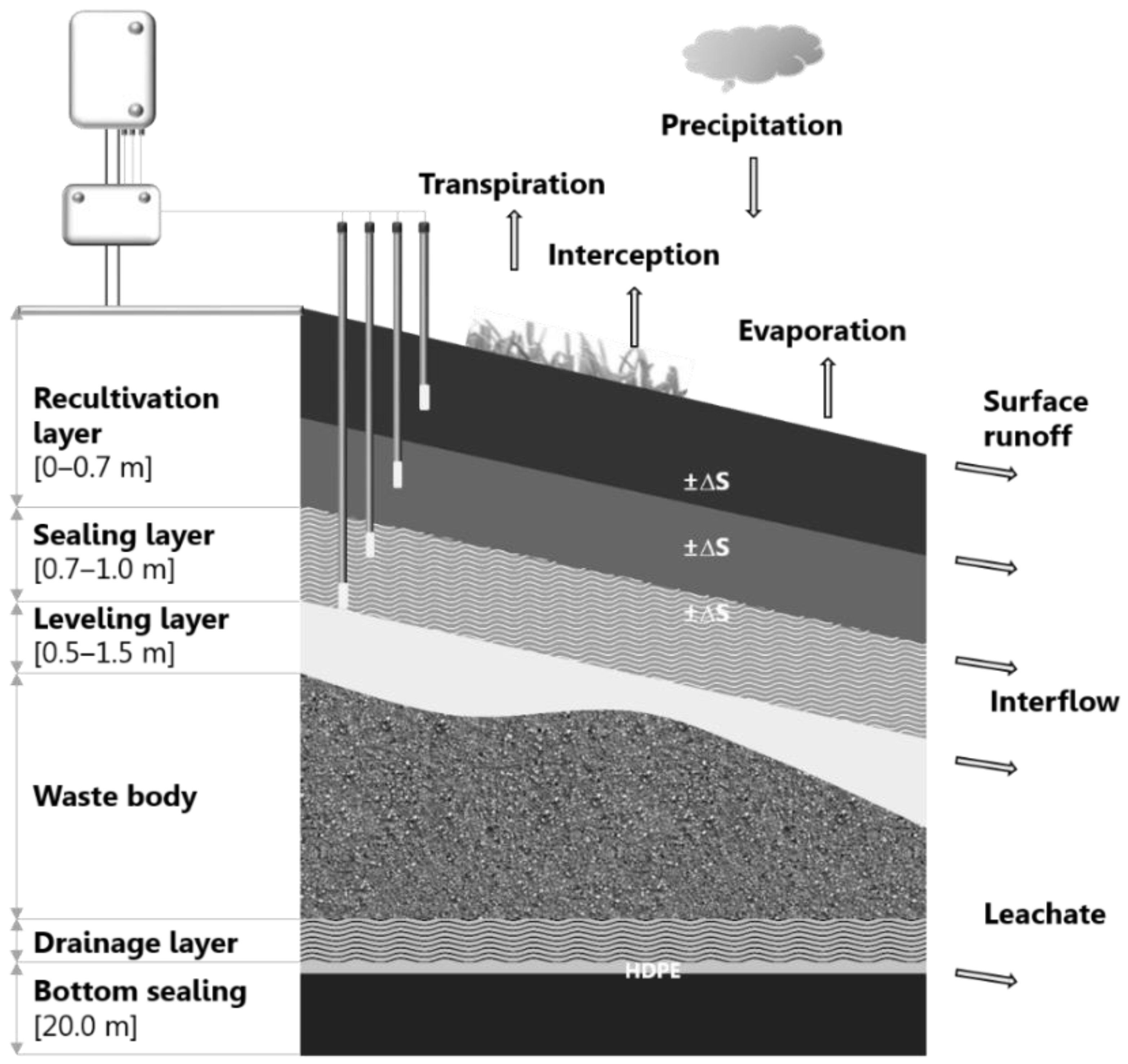
The influence of exposure and slope gradient on global solar radiation and therefore (a) potential and actual evapotranspiration (ETp, ETa), (b) θ_EZ, and (c) outflow and leachate were determined on the basis of the input data for the HELP model as mentioned before. In 2012, the ETp_uncorr. and ETa_uncorr. values of area I were up to 67 mm/year and 30 mm/year higher than the ETa_corr. values and the difference decreased to 52 mm/year and 12 mm/year in 2014, respectively. On the other hand, for areas II and III there were smaller differences, between 13 mm/year and 32 mm/year, or 0.79 mm/year and 5.43 mm/year, respectively, with comparatively higher ETp_corr. and ETa_corr. values due to surface area factors > 1 (Figure 2).

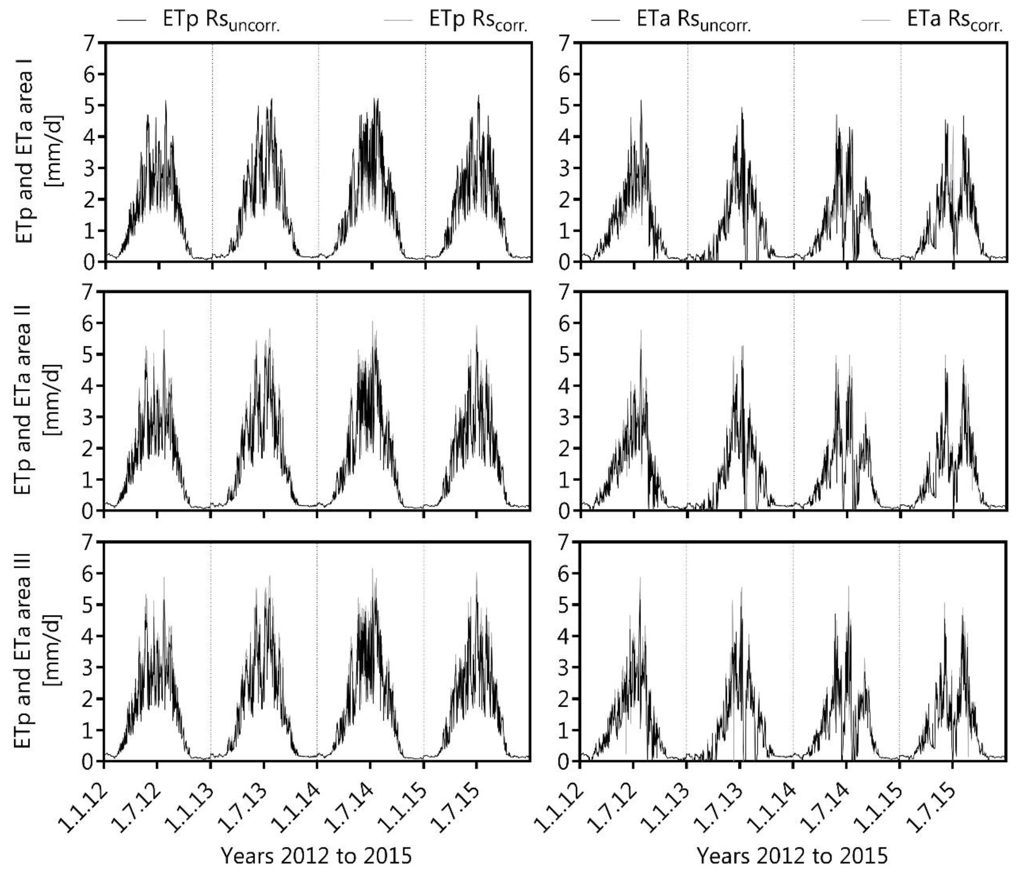
The maximum depth of the evaporative zone was 0.5 m and complied with the part of the recultivation layer (0–0.7 m) in which water content fluctuated relatively intensely during the study period (Figure 3). Area II, with southwest exposure and the highest slope gradients, showed the highest ETa values of up to 5.87 mm/d, but also more pronounced phases during the vegetative period where the θ_EZ are lower than the wilting point, resulting in higher discrepancies between ETp and ETa of up to 6 (corr.) and 5.3 mm/d (uncorr.).

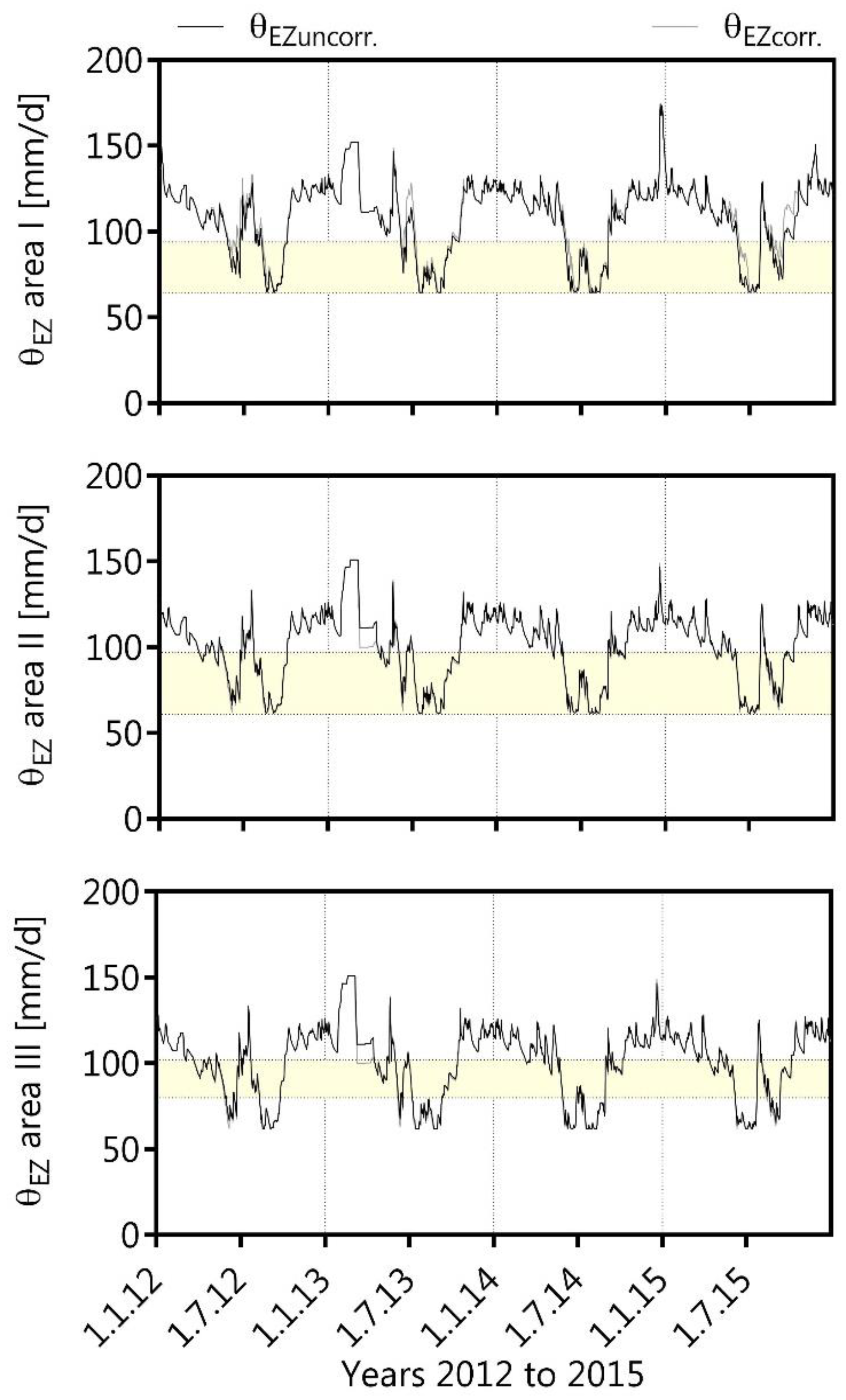
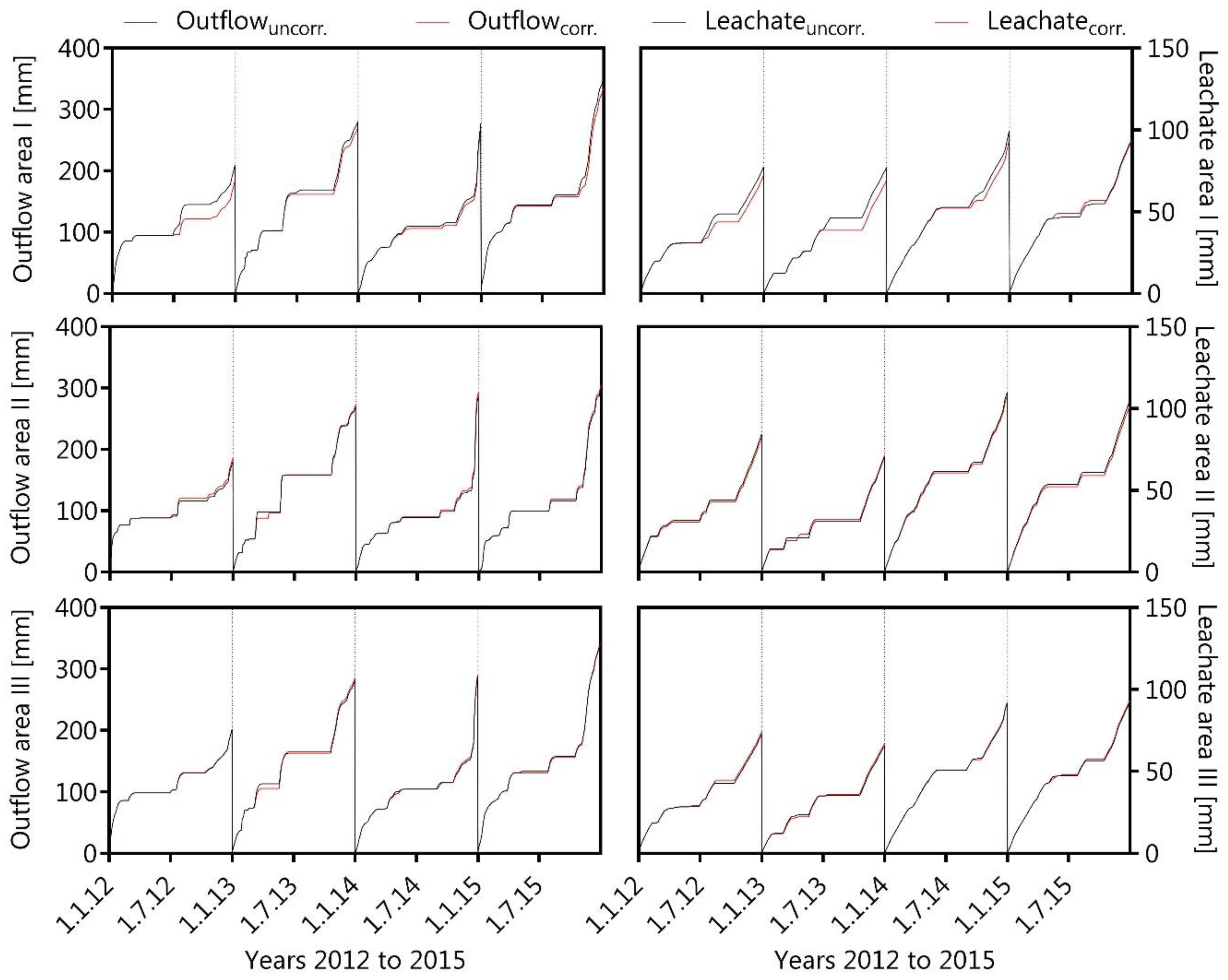
The areas I and III showed the highest discrepancies between cumulative corr. and uncorr. modeled outflow rates of up to 47 mm/year in 2015, while area II showed moderate discrepancies between 9 mm/year and 17 mm/year, with higher total uncorr. outflow rates. The highest differences between cumulative corr. and uncorr. leachate rates were also determined for area III in 2012, with 18 mm/year, while Area II showed the smallest differences, between 0.41 mm/year and 3.5 mm/year (Figure 4).

3.5. Observation and Modeling Results

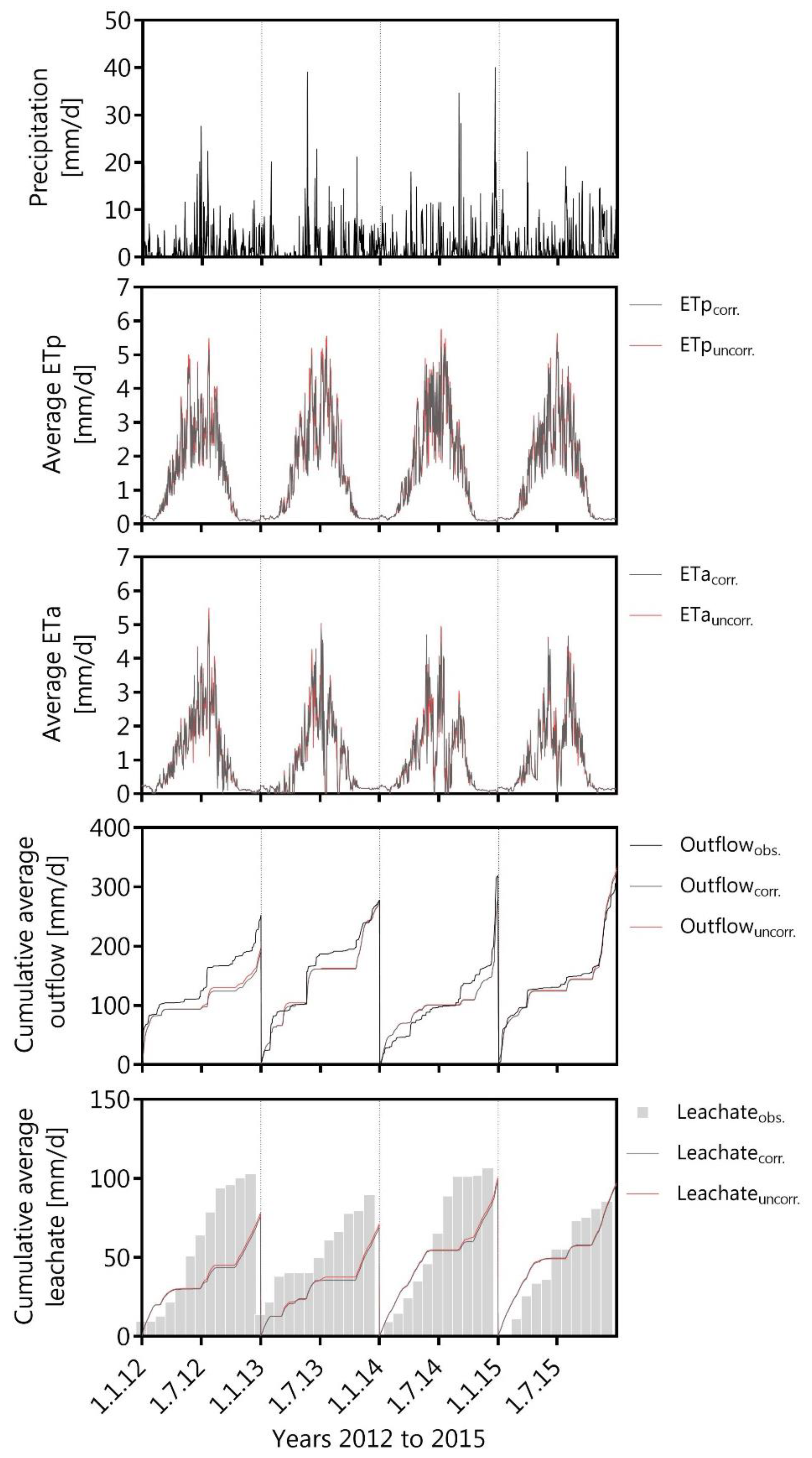
In the period between 2012 and 2015, nearly 59–64% of annual precipitation fell in the hydrological summer period (November 1 to April 30), and 36–41% in the hydrological winter period (May 1 to October 31). In contrast, the more humid years 2014 and 2015, with 753 and 767 mm, respectively, are characterized by approximately equally distributed precipitation rates in the winter period (52–54%) and in the summer period (46–48%). The years 2012 and 2013 showed lower annual precipitation rates, with 655 mm and 669 mm, respectively, compared to the average annual precipitation rate of 752 mm (Figure 5). The winters from 2012 to 2015 were mostly mild and only had some snow. The corr. and uncorr. water balance components enable the comparison between the modeled outflow and the leachate rates with the observed ones.

The corr. and uncorr. averaged ETp values showed small differences, between 2 mm/year in 2012 and 11 mm/year in 2014. Therefore, the corr. ETa values are in total higher than the uncorr. ETa values, with differences between 1.6 mm/year in 2014 and 8.3 mm/year in 2012. Additionally, drier phases between June and September were regularly characterized by higher discrepancies between ETp values and ETa values of up to 4.9 mm/d and 6.1 mm/d. On the other hand, the early warming phase during March to May showed moderate discrepancies of 0.58 mm/d to 2.76 mm/d, and, during October to February of the following year, mostly no discrepancies were found.

Outflow was estimated as the sum of the surface runoff and interflow; thus, the uncorr. outflow values were negligibly higher than the corr. values (Figure 5). Therefore, the modeled outflow values were averaged due to the different slope gradients and spatial inhomogeneity of areas I, II, and III. As a result, the average annual outflow varied proportionally between 38–42% (observed) and 30–43% (modeled) of the annual precipitation, while the average surface runoff varied proportionally between 0.2–12% of the outflow (Figure 5). Additionally, the adequate dimensioning of the drainage layer can be attributed to the average annual damming height that differed between 36–62 mm for area I, 9–15 mm for area II, and 33–56 mm for area III.

Furthermore, the corr. and uncorr. leachate rates could also be neglected, and the comparatively increased leachate rates in 2012 and 2014 could be attributed to maintenance services of the leachate pipelines, where the landfill was almost completely pumped out. Excluding the year 2013, the period from April to September of each year was predominantly associated with approximately 73–80% of the observed, but only 20–28% of the modeled leachate rate. Altogether, the highest leachate rates were modeled between the more humid months of November, December, January, and February, even though the summer leachate rates, due to intensive precipitation events, were partially underestimated. As a result, the observed leachate rates could only be used to a limited extent to describe the modeled leachate rates (Figure 5).

3.6. Water Balance of the Rastorf Landfill

In the study period between 2012 and 2015, climatic water balance was positive (precipitation > evapotranspiration) and, with regard to German weather conditions, the ETa was the greatest output value of the water balance (

Table 9. Observed (obs) and average simulated (mod) water-balance components of the temporary capping system between 2012 and 2015 in mm/year. The ± symbol corresponds to standard deviation.

Water Balance (mm/year)	2012		2013		2014		2015
	mod	obs	mod	obs	mod	obs	mod	obs
Precipitation	655	655	670	670	753	753	767	767
Actual evapotranspiration *	383 ± 6	300	328 ± 2	303	358 ± 1	328	357 ± 4	374
Outflow **	193 ± 5	252	277 ± 1	278	283 ± 1	318	329 ± 3	308
∆ soil moisture content	1.54	3.9	−4.7	0.4	11.5	−5.2	−17.5	−3.3
Leachate	77 ± 2	103	70 ± 2	89	98 ± 2	106	97 ± 1	85

* including interception loss, residual value for observed data, ** surface runoff, and lateral drainage.

). In a last step, the corr. and uncorr. ETa values, outflow and leachate rates were averaged for the study period to statistically compare the observed and modeled water balance components. The observed and modeled average annual ETa values ranged between 44% and 48%, and the lateral drainage rates between 38% and 43% of the annual precipitation. An exception is the year 2012 with a modeled ETa value of 383 mm (58% of the precipitation) compared to the observed value of 300 mm in 2012, while the modeled outflow of 193 mm (30% of the precipitation) is comparatively lower than the observed value of 252 mm. The change in soil-moisture content was moderate, but the modeled value increased in the more humid year 2014 compared to 2012 or 2013, and decreased significantly in 2015. The observed leachate rates varied slightly, between 11.2% and 13.3% of annual precipitation, while the modeled leachate rates ranged from 11.1% to 15.7% of annual precipitation (Table 9).

3.7. Statistical Analysis and Model Accuracy

The Nash–Sutcliffe efficiencies of the individual monthly values of actual evapotranspiration varied between −2.7 and 0.19 with an RMSE of 20.42 to 26.21; RSR values varied between 0.9 and 1.91. In contrast, the cumulative monthly values were characterized by higher NSE values between 0.62 and 0.91 with an RMSE of 40.14 to 83.78; RSR values differed between 0.28 in 2015 and 0.69 in 2012 (

Table 10. Results of the statistical analysis based on the comparison between the averaged observed and modeled actual evapotranspiration rates between 2012 and 2015.

	Actual Evapotranspiration *
Year	2012	2013	2014	2015
Individual values
RMSE (mm)	20.42	23.96	22.64	26.21
NSE (-)	0.19	0.20	−2.7	−0.24
RSR (-)	0.90	0.86	1.91	1.01
Cumulative values
RMSE (mm)	83.78	64.98	52.41	40.14
NSE (-)	0.62	0.75	0.76	0.91
RSR (-])	0.69	0.52	0.49	0.28

* average of area I, II, and III.

).

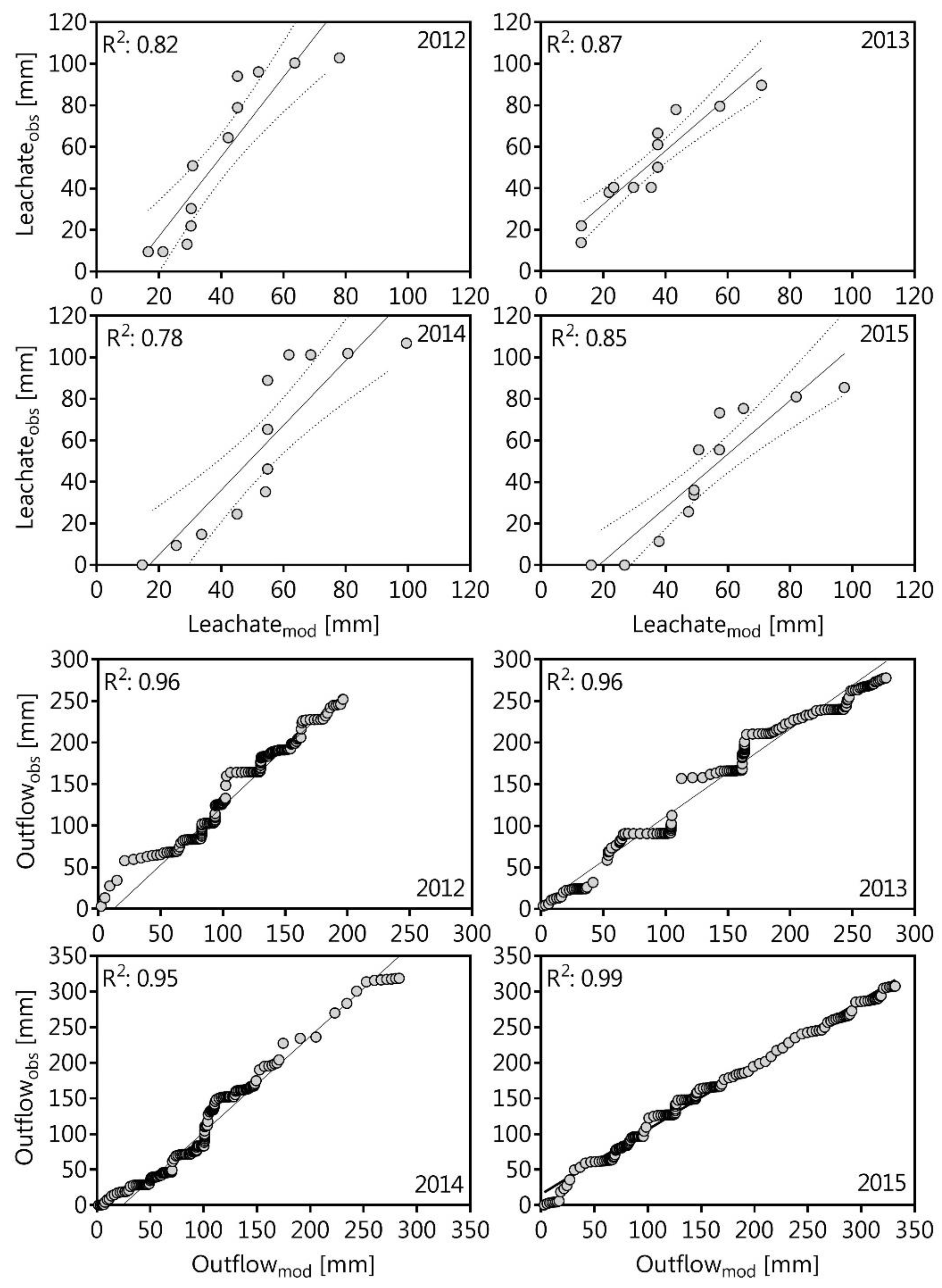
The positive Nash–Sutcliffe efficiencies of the average annual outflow varied between 0.14 and 0.39 with an RMSE of 1.67 mm to 2.61 mm. Otherwise, the RMSE of the annual leachate differed between 7.27 mm in the year 2013 and 10.3 mm to 12.1 mm in the remaining years, with negative NSE values. RSR values differed, from 1.3 in 2013 to 1.63 in 2014. However, the cumulative average annual outflow rates were characterized by higher NSE values between 0.64 and 0.93, with an RMSE of 18.95 mm to 31.75 mm, while RSR values varied between 0.32 in 2015 and 0.7 in 2012. Otherwise, the monthly-based leachate rates were characterized by negative NSE values between −0.74 and −1.49 and RSR values > 1.3, while the cumulative values indicate NSE > 0.37 up to 0.73 in 2015 and RSR < 0.87. (

Table 11. Results of the statistical analysis based on the comparison between the averaged observed and modeled outflow and leachate rates between 2012 and 2015.

	Outflow *				Leachate *
Year	2012	2013	2014	2015	2012	2013	2014	2015
Individual values
RMSE (mm)	2.01	2.6	2.25	1.67	10.35	7.40	12.12	11.06
NSE (-)	0.14	0.23	0.39	0.29	−1.34	−0.74	−1.70	−1.49
RSR (-)	0.93	0.87	0.78	1.20	1.57	1.30	1.63	1.51
Cumulative values
RMSE (mm)	31.7	20.0	21.4	18.9	29.6	21.3	24.7	16.3
NSE (-)	0.64	0.92	0.87	0.93	0.48	0.37	0.64	0.73
RSR (-)	0.70	0.29	0.37	0.32	0.75	0.87	0.62	0.50

* average of Area I, II, and III.

). The regression analysis of the observed and modeled outflow data indicated an R² between 0.95 and 0.99, while the leachate data varied with an R² of 0.78 to 0.87 in 2015 (Figure 6).

4. Discussion

4.1. Plausibility of the Observed and Modeled Water-Balance Components

In the first step, sensitivity analysis and the calibration phase were carried out with the weather data between 2008 and 2011 to improve the model performance (i.e., error tolerance) as described in the literature [19,37,38]. Moreover, the Ks values of the drainage layer strongly influenced the outflow rates, while the Ks values of the barrier soil layer were of major importance for the leachate rates. Thus, the Ks values of the calibration alternative were fitted compared to the observed Ks values of the zero alternative as also detailed described in the literature [38].

In the second step, the validation phase was necessary to evaluate the quality of the model performance [14,31]. Therefore, the validity of the modeling results depends on the quality of the input data and related measurement methods that exhibit random errors [43] depending on site and weather conditions.

The observed annual precipitation rates between 655 mm and 767 mm were plausible compared to the long-term average precipitation rate in the study area of 752 ± 186 mm between 1991 and 2015. Thus, the uncorrected precipitation data were used as input parameters for the HELP model as mentioned in the literature [30]. It should be kept in mind that the observed precipitation data could be underestimated by up to 17% [25,44], caused by wetting failures and wind-induced precipitation losses [45].

The ETa values in Central Europe for grassland vegetation with a good stand vary in the range of 450–550 mm/year [46], considering a precipitation rate of 700–800 mm/year (i.e., Rastorf landfill). Therefore, the observed and modeled ETa values ranging between 300 mm/year and 383 mm/year were also significantly smaller than those described in the literature [10,47] for approx. comparable weather conditions in Northern Germany (NG). This discrepancy can be explained by the dense installation of the recultivation layer resulting in root depths at a maximum of 0.35 m to 0.4 m and therefore limited transpiration capacity, as mentioned in the literature [48]. The HELP model also assumed a constant LAI of 3.5 m²/m², underestimating the transpiration performance during the vegetative period [30]. Furthermore, the observed interception was determined according to a method in the literature [22], which included a risk of potential underestimation of the interception performance. The corrected Rs values showed pronounced southeast or southwest exposure [49], while ETp, ETa, and θ_EZ were strongly affected.

The observed outflow data varied between 252 mm/year and 318 mm/year, though surface runoff and lateral drainage could technically not be separated. The modeled surface runoff was a very minor component (<10 mm/year) due to the good stand of the grass at the surface of the recultivation layer, as mentioned in the literature [5,6,47]. Additionally, snowmelt or precipitation on frozen soil, leading to an overestimation of the surface runoff over longer periods [31], did not affect the results under the given weather conditions. Moreover, discrepancies between observed and modeled outflow data could also be attributed to technical defects of the V-notch weirs. Thus, linear regression analysis was used to complete the missing outflow data.

The observed leachate rates between 85 mm/year and 106 mm/year, or 11.1–15.7% of the annual precipitation exceeded the regulatory limit of 60 mm/year by five years after construction at the latest [8]. Thus, the varying leachate rates between 2012 and 2015 can be explained by the maintenance services of the leachate pipelines (see Section 3.5).

Leachate generation was strongly influenced by the seasonality of the precipitation, and the estimated leachate rates indicate a sufficient percolation of water into the waste body to support microbial processes [9]. Therefore, the settlements of the waste body decreased from > 20 cm/year to < 4 cm/year between 2008 and 2017. Thus, the semipermeable system fulfills its purpose.

The slightly varying annual leachate rates indicate the functionality of the temporary capping system. Continuously rising leachate rates would be an indicator of shrinkage crack formation or root penetration in the sealing layer [47,49]; thus, the capping system would be ineffective.

4.2. Comparison of Observed and Modeled Water Balance Components

The modeled water-balance components were tested considering variations in global solar radiation as mentioned before and then averaged for the following balancing. As a first step, the observed annual precipitation rates served as unchanged input data for the HELP model. The wetter year 2011, with 760 mm precipitation, was characterized by a final soil-moisture content of 251 mm (initial water content in 2012) as stated in the literature [7]. Thus, the model assumed a final soil-moisture content of 267.9 mm in 2012, despite only 655 mm/year precipitation; so, θ_EZ was overestimated, resulting in a modeled ETa of 379 mm compared to 300 mm observed.

Between 2013 and 2015, annual observed and modeled ETa values corresponded to a maximum of 48% of annual precipitation. The differences can be explained by the maximum LAI, which strongly influenced the evapotranspiration rate [2], while the HELP model assumed a constant LAI of 3.5 m²/m², as mentioned before. Moreover, the daily average wind speed values did not reflect the actual wind conditions of an entire day [50]. Thus, the evaporative capacity of the wind-exposed Rastorf landfill must also be regarded as underestimated.

Additionally, the evaporative zone of the Rastorf landfill dried out strongly during the drier summer months as mentioned in the literature [49]. Thus, the transpiration capacity of the grassland was restricted by (a) inadequate water availability in the evaporative zone, (b) limited water-storage capacity, and (c) limited capillary rise from deeper soil layers due to compacted installation [7]. Therefore, periods with water content in the evaporative zone below the critical FC value of 95 mm should be as short as possible to prevent desiccation in the deeper layer. So, it should be kept in mind that the modeled water content is a first indicator to describe the hydraulic stability of the capping system.

The surface runoff in Figure 6 (0.2–12% of the outflow) is less pronounced than the modeled lateral drainage rates between 38% and 43% of the annual precipitation, excluding the 30% in 2012. Thus, the surface runoff increased with increasing curve number based on slope length and gradient (area III > II > I). It must be considered that the SCS precipitation–runoff relation probably underestimated the runoff on a daily basis, especially when the precipitation duration was very short and the intensity was very high [51]. The quasi-unsteady approach of a vertical flow into the drainage layer and a stationary one-dimensional saturated drainage flow could lead to changing flow rates from one time step to another [25]. This circumstance can result in a muted drainage rate and, thus, in a delayed increase and decrease of the drainage rate (i.e., 2012) during drainage events [10].

Additionally, the observed leachate rates were strongly delayed in time, resulting in differences between the observed and modeled values, because the leachate rates could only be determined by the actually cleaned quantities. The soil water dynamics during the seasonal drying and wetting regime of the temporary capping system of the Rastorf landfill was described in the following literature [1]. Therefore, the barrier soil layer (0.7–1.0 m) never dried out due to water contents ≥ 0.278 m³/m³. So, the barrier soil layer displayed nearly saturated conditions, especially during the humid winter months. In this case, the calculated annual leachate rates were directly connected to the volume of water ponding on and also stored in the barrier soil layer due to the bottom boundary condition of the HELP model, based on the saturated Darcy flow [25].

It should also be considered that the role of the waste body should usually not be neglected in explaining the differences between observed and modeled leachate data. However, municipal solid waste is very heterogeneous and poorly compacted; thus, particles of geosynthetics and geotextiles can channel the drainage or restrict the wetting of the waste [25]. The amount of water used by effective microorganisms should decrease in time and, therefore, the amount of water stored and also used in the waste body [52]. However, the role of the waste body was also neglected due to missing field data to quantify the changes in the water content from the initial phase until today.

4.3. Statistical Comprehension of Observed and Modeled Water-Balance Components

The statistical agreement between the observed and modeled outflow (R²: 0.95–0.99) and leachate data (R²: 0.78–0.87) indicates an acceptable validation over the range of the Rastorf landfill constituents, which were modeled according to the literature [39,43]. In all successfully verified cases, the obtained R² values were higher than 0.5, and the RMSE values were also acceptable according to thresholds described by the literature [43]. Modeling results can be judged as satisfactory if the NSE values were higher than 0.5, and the RSR values lower than 0.7 as cited in the literature [41]. Based on NSE and R² values close to 1, RMSE, and small RSR values, the HELP model performed much better for cumulative values than individual ones as also mentioned in the literature [39]. The differences can mainly be explained by huge disparities between the daily or monthly observed and modeled data (i.e., outflow on 5 October 2012: observed: 23.84 mm, modeled: 6.14 mm); statistical outliers had a disproportionate impact on forecast quality [40].

4.4. Limitations of the Modeling Approach

In our analysis, we assumed static soil conditions to establish the modeling process [30], but structure formation processes could be attributed to swell shrink and biological processes over time, which can be also explained by the in situ matric potential dynamics [1], resulting in possible changes of water-storage capacity [49]. Furthermore, aging or drying of the mineral layer would also not be considered, so the Ks value did not vary during the complete period. Additionally, processes like waste aging and compression were not recognized by the HELP model and may affect the leachate prediction, resulting in an underestimation of the leachate generation [3]. In case of evapotranspiration, tree species or shrub vegetation (i.e., Salix caprea, Ligustrum vulgare) would be more effective than grassland, but vegetation types with LAI values greater than 5 m²/m² cannot be sufficiently considered by the HELP model [31]. It should also be kept in mind that deep-rooting trees or shrub vegetation could adversely affect the hydraulic stability of landfill liners. However, it is well known that the observed ETa values primarily depend on the size of the mentioned errors of the precipitation data and outflow [7].

On the other hand, there is also no automatic correction of the global solar radiation due to exposure and slope gradient; thus, this step should be carried out separately before the simulation run. The HELP model also underestimates the influence of the leaf area index, structure, and evaporative zone depth and, therefore, the actual evapotranspiration, which was also already described in the literature [30].

5. Conclusions

For this study, the HELP model was applied as one of the most commonly used statistical-empirical approaches to predict the water-balance components of landfill capping systems, and several conclusions could be drawn from our findings. The modeling results were realistic reflecting observed outflow and leachate data, even with a limited set of input data.

The surface area factor v strongly affected the evapotranspiration rates of the southeast- and southwest-exposed areas II and II considering the corrected global solar radiation. This correction step was necessary and should be implemented in the model routine, in particular for landfills with pronounced exposure in the southern direction and distinct slope gradients.

Irrespective of these results, the authors are aware that the assumed modeling simplifications and possible errors may cause modeling uncertainties. Thus, it should be considered that valid input data are absolutely necessary for the success of the simulation run. Additional sensitivity analysis is also essential to determine the influence of individual factors on the modeling result.

In summary, the HELP model allowed to prove the functionality of a temporary capping system under the given weather and site conditions. In order to finally validate the water fluxes in mineral capping systems, more physically based models could give more insight into the variations in soil water characteristics. This step will be part of further research, as well as leachate composition and its impact on the environment.

References

- Beck-Broichsitter, S.; Fleige, H.; Horn, R. Waste capping systems processes and consequences for the longterm impermeability. In Soils within Cities; Levin, M., Kim, H.J., Morel, J.L., Burghardt, W., Charzynski, P., Shaw, R.K., Eds.; Catena Soil Sciences: Stuttgart, Germany, 2018; pp. 148–152. [Google Scholar]
- Hauser, V.L. Evapotranspiration Covers for Landfills and Waste Sites; CRC Press, Taylor and Francis: Boca Raton, FL, USA, 2008. [Google Scholar]
- Pantini, S.; James Law, H.; Verginelli, I.; Lombardi, F. Predicting and comparing infiltration rates through various landfill cap systems using water-balance models—A case study. In Proceedings of the 2013 ISWA World Congress, Vienna, Austria, 7–11 October 2013. [Google Scholar]
- Simon, F.G.; Müller, W.W. Standard and alternative landfill capping design in Germany. Environ. Sci. Policy 2004, 7, 277–290. [Google Scholar] [CrossRef]
- El Kateb, H.; Zhang, H.F.; Zhang, P.C.; Mosandl, R. Soil erosion and surface runoff on different vegetation covers and slope gradients: A field experiment in Southern Shaanxi Province, China. Catena 2013, 105, 1–10. [Google Scholar] [CrossRef]
- Zhang, L.; Wang, J.; Bai, Z.; Lu, C. Effects of vegetation on runoff and soil erosion on reclaimed land in an opencast coal-mine dump in a loess area. Catena 2015, 128, 44–53. [Google Scholar] [CrossRef]
- Widomski, M.K.; Beck-Broichsitter, S.; Zink, A.; Fleige, H.; Horn, R. Numerical modeling of water balance for temporary landfill cover in North Germany. J. Plant Nutr. Soil Sci. 2015, 178, 401–412. [Google Scholar] [CrossRef]
- German Landfill Directive. Degree on landfills (ordinance to simplify the landfill law). In The Form of the Resolution of the Federal Cabinet; Federal Ministry of the Environment, Nature Conservation: Bonn, Germany, 2009. [Google Scholar]
- Rowe, R.K. Systems engineering: The design and operation of municipal solid waste landfills to minimize contamination of groundwater. Geosynth. Int. 2011, 18, 391–404. [Google Scholar] [CrossRef]
- Berger, K. On the current state of the Hydrologic Evaluation of Landfill Performance (HELP) model. Waste Manag. 2015, 38, 201–209. [Google Scholar] [CrossRef] [PubMed]
- Pantini, S.; Verginelli, I.; Lombardi, F. A new screening model for leachate production assessment at landfill sites. Int. J. Environ. Sci. Technol. 2014, 11, 1503–1516. [Google Scholar] [CrossRef]
- Yang, N.; Damgaard, A.; Kjeldsen, P.; Shao, L.-M.; He, P.-J. Quantification of regional leachate variance from municipal solid waste landfills in China. Waste Manag. 2015, 46, 362–372. [Google Scholar] [CrossRef] [PubMed] [Green Version]
- Diersch, H.J.G. FEFLOW, Finite Element Subsurface Flow and Transport Simulation System Reference Manual; DHI-WASY Ltd.: Berlin, Germany, 2002. [Google Scholar]
- Šimůnek, J.; van Genuchten, M.T.; Sejna, M. HYDRUS: Model use, calibration and validation. Special issue on Standard/Engineering Procedures for Model Calibration and Validation. Trans. ASABE 2012, 55, 1261–1274. [Google Scholar]
- Schäffer, B.; Schulin, R.; Boivin, P. Changes in shrinkage of restored soil caused by compaction beneath heavy agricultural machinery. Eur. J. Soil Sci. 2008, 59, 771–783. [Google Scholar] [CrossRef]
- Hartge, K.H. Ein Haubenpermeameter zum schnellen Durchmessen zahlreicher Stechzylinderproben. Z. Kulturtech. Flurbereinigung 1966, 7, 155–163. [Google Scholar]
- Hartge, K.H.; Horn, R. Essential Soil Physics—An Introduction to Soil Processes, Structure, and Mechanics; Horton, R., Horn, R., Bachmann, J., Peth, S., Eds.; Schweizerbart Science Publishers: Stuttgart, Germany, 2016. [Google Scholar]
- Allen, R.G.; Smith, M.; Perrier, A.; Pereira, L.S. An update for the calculation of reference evapotranspiration. ICID Bull. 1994, 43, 35–92. [Google Scholar]
- Allen, G.A.; Pereira, L.S.; Raes, D.; Smith, M. Crop Evapotranspiration—Guidelines for Computing Crop Water Requirements; No. 56; FAO Irrigation and Drainage Papers: Rome, Italy, 1998. [Google Scholar]
- Unger, H.; Skiba, M. Solare Strahlung auf geneigte Flächen. Sonnenenergie 1998, 1/98, 48–50. [Google Scholar]
- Merkblatt ATV-DVWK-M 504. Verdunstung in Bezug zu Landnutzung, Bewuchs und Boden; GFA-Gesellschaft zur Förderung der Abwassertechnik e.V.: Hennef, Germany, 2002. [Google Scholar]
- Hoyningen-Huene, J.F.V. Die Interzeption des Niederschlags in landwirtschaftlichen Pflanzenbeständen. Schriftenr. Dtsch. Verb. Wasserwirtsch. Kulturbau 1983, 57, 1–53. [Google Scholar]
- Schroeder, P.R.; Dozier, T.S.; Zappi, P.A.; McEnroe, B.M.; Sjostrom, J.W.; Peyton, R.L. The Hydrologic Evaluation of Landfill Performance (HELP) Model. Engineering Documentation for Version 3. EPA/600/R-94/168b; US Environmental Protection Agency: Cincinnati, OH, USA, 1994.
- Ad-Hoc-AG Boden. Bodenkundliche Kartieranleitung (Soil Survey Manual), 5th ed.; Bundesanstalt für Geowissenschaften und Rohstoffe in Zusammenarbeit mit den Staatlichen Geologischen Diensten der Bundesrepublik Deutschland: Hannover, Germany, 2005. [Google Scholar]
- Berger, K.; Schroeder, P.R. The Hydraulic Evaluation of Landfill Performance Model. Version HELP 3.95 D. Software and Electronic Documents as PDF: User’s Guide; Supplement to the Engineering Documentation of HELP 3.07; Institute of Soil Science, University of Hamburg: Hamburg, Germany, 2013; Available online: http://www.geo.uni-hamburg.de/en/bodenkunde/service/help-model.html (accessed on 11 March 2015).
- Penman, H.L. Vegetation and Hydrology; Technical Comment No. 53; Commonwealth Bureau of Soils: Harpenden, UK, 1963. [Google Scholar]
- Arnold, J.G.; Williams, J.R.; Nicks, A.D.; Sammons, N.B. SWRRB, A Basin Scale Simulation Model for Soil and Water Resources Management; Texas A and M University Press: College Station, TX, USA, 1990. [Google Scholar]
- Ritchie, J.T. A model for predicting evaporation from a row crop with incomplete cover. Water Resour. Res. 1972, 8, 1204–1213. [Google Scholar] [CrossRef]
- Sharpley, A.N.; Williams, J.R. EPIC—Erosion/Productivity Impact Calculator: 1. Model Documentation; Report PB91-136119; US Department of Agriculture: Washington, DC, USA, 1990.
- Berger, K. Potential and limitations of applying HELP model for surface covers. Pract. Period. Struct. Des. Constr. 2002, 6, 192–203. [Google Scholar] [CrossRef]
- Berger, K. Validation of the Hydrological Evaluation of Landfill Performance (HELP) model for simulating the water balance of cover systems. Environ. Geol. 2000, 39, 1261–1274. [Google Scholar] [CrossRef]
- Campbell, G.S. A simple method for determining unsaturated hydraulic conductivity from moisture retention data. Soil Sci. 1074, 117, 311–314. [Google Scholar] [CrossRef]
- Brooks, R.H.; Corey, A.T. Hydraulic Properties of Porous Media; Hydrology Paper No. 3; Colorado State University: Fort Collins, CO, USA, 1964. [Google Scholar]
- Forchheimer, P. Hydraulik, 3rd ed.; Teuber: Leipzig, Germany; Berlin, Germany, 1930. [Google Scholar]
- USDA (Soil Conservation Service). National Engineering Handbook, Section 4, 115 Hydrology; US Government Printing Office: Washington, DC, USA, 1985.
- Soulis, K.X.; Valiantzas, J.D. SCS-CN parameter determination using rainfall-runoff data in heterogeneous watersheds—The two-CN system approach. Hydrol. Earth Syst. Sci. 2012, 16, 1001–1015. [Google Scholar] [CrossRef] [Green Version]
- Berger, K. Validierung und Anpassung des Simulationsmodells HELP zur Berechnung des Wasserhaushalts von Deponien für Deutsche Verhältnisse; Umweltbundesamt: Berlin, Germany, 1998. [Google Scholar]
- Budde, J. Empirischer Vergleich komplexer Methoden zur Bestimmung von Wasserhaushaltskenngrößen einer Oberflächenabdichtung am Beispiel der Deponie Rastorf (Schleswig-Holstein). Master’s Thesis, Christian Albrechts University, Kiel, Germany, 8 February 2016. [Google Scholar]
- Moriasi, D.N.; Arnold, J.G.; Van Liew, M.W.; Binger, R.L.; Harmel, R.D.; Veith, T.L. Model evaluation guidelines for systematic quantification of accuracy in watershed simulations. Trans. ASABE 2007, 50, 885–900. [Google Scholar] [CrossRef]
- Chai, T.; Draxler, R.R. Root mean square error (RMSE) or mean absolute error (MAE)? Arguments against avoiding RMSE in the literature. Geosci. Model Dev. Dis. 2014, 7, 1247–1250. [Google Scholar] [CrossRef]
- Golmohammadi, G.; Prasher, S.; Madani, A.; Rudra, R. Evaluating three hydrological distributed watershed models: MIKE-SHE, APEX, SWAT. Hydrology 2014, 1, 20–39. [Google Scholar] [CrossRef]
- Nash, J.E.; Sutcliffe, J.V. River flow forecasting through conceptual models part I—A discussion of principles. J. Hydrol. 1970, 10, 282–290. [Google Scholar] [CrossRef]
- Singh, J.; Knapp, H.V.; Demissie, M. Hydrologic Modeling of the Iroquois River Watershed Using HSPF and SWAT. J. Am. Water Resour. Assoc. 2004, 41, 343–360. [Google Scholar] [CrossRef]
- Gebler, S.; Hendricks Franssen, H.-J.; Pütz, T.; Post, H.; Schmidt, M.; Vereecken, H. Actual evapotranspiration and precipitation measured by lysimeters: A comparison with eddy covariance and tipping bucket. Hydrol. Earth Syst. Sci. 2015, 19, 2145–2161. [Google Scholar] [CrossRef] [Green Version]
- Richter, D. Ergebnisse Methodischer Untersuchungen zur Korrektur des Systematischen Messfehlers des Hellmann-Niederschlagsmessers; Deutscher Wetterdienst: Offenbach, Germany, 1995. [Google Scholar]
- GDA-Empfehlung E2-32. Gestaltung des Bewuchses auf Deponien, Published in January 2010. Available online: http://www.gdaonline.de (accessed on 22 February 2018).
- Melchior, S.; Sokollek, V.; Berger, K.; Vielhaber, B.; Steinert, B. Results from 18 Years of in situ performance testing of landfill cover systems in Germany. J. Environ. Eng. ASCE 2010, 136, 815–823. [Google Scholar] [CrossRef]
- Beck-Broichsitter, S.; Fleige, H.; Horn, R. Compost quality and its function as a soil conditioner of recultivation layers—A critical review. Int. Agrophys. 2018, 32, 11–18. [Google Scholar] [CrossRef]
- Horn, R.; Stępniewski, W. Modification of mineral liner to improve its long-term stability. Int. Agrophys. 2004, 18, 317–323. [Google Scholar]
- Pereira, L.S.; Allen, R.G.; Smith, M.; Raes, D. Crop evapotranspiration estimation with FAO56: Past and future. Agric. Water Manag. 2015, 147, 4–20. [Google Scholar] [CrossRef]
- Lilly, A. The relationship between field-saturated hydraulic conductivity and soil structure: Development pf class pedotransfer functions. Soil Use Manag. 2000, 16, 56–60. [Google Scholar] [CrossRef]
- Öncü, G.; Reiser, M.; Kranert, M. Aerobic in situ stabilization of Landfill Konstanz Dorfweiher: Leachate quality after 1 year of operation. Waste Manag. 2012, 32, 2374–2384. [Google Scholar] [CrossRef] [PubMed]
Figure 1.
Schematic cross section through the Rastorf landfill including water-balance components (Equation (1)) and installation positions of in situ measurement devices (tensiometers, FDR sensors) in 0.2, 0.5, 0.8, and 1.0 m depth; HDPE: high-density polyethylene; interception (I): interception loss (I-evaporation).
Figure 2.
Modeled potential (ETp) and actual evapotranspiration (ETa) with corrected (corr.) and uncorrected (uncorr.) global solar radiation (Rs) between 2012 and 2015 for Areas I, II, and III.
Figure 3.
Average water content in the evaporative zone (0.5 m) between 2012 and 2015 for Areas I, II, III. The dashed lines indicate the area between the FC and WP.
Figure 4.
Modeled averaged cumulative outflow (sum of surface runoff and lateral drainage) leachate rates for areas I, II, and III between 2012 and 2015.
Figure 5.
Observed and modeled averaged water-balance components: precipitation, corr. and uncorr. potential and actual evapotranspiration (ETp, ETa), outflow (sum of surface runoff and lateral drainage), and leachate.
Figure 6.
Linear regression analysis of the comparison between observed and simulated leachate and outflow data (dots) for the years 2012 (upper left), 2013 (upper right), 2014 (lower left), and 2015 (lower right). R2 indicates the coefficient of determination, and the dashed lines indicate the confidence limits for a confidence level of 95%.