Combined Gravimetric-Seismic Moho Model of Tibet


1
Schmidt Institute of Physics of the Earth, Russian Academy of Sciences, Moscow 119991, Russia
2
Institute of Earthquake Prediction Theory and Mathematical Geophysics, Russian Academy of Sciences, Moscow 119991, Russia
3
Division of Geodesy and Geoinformatics, Royal Institute of Technology (KTH), 114 28 Stockholm, Sweden
4
Department of Industrial Development, IT and Land Management, University of Gävle, 801 76 Gävle, Sweden
5
Department of Land Surveying and Geo-Informatics, Hong Kong Polytechnic University, Hong Kong, China
*
Author to whom correspondence should be addressed.
Geosciences 2018, 8(12), 461; https://doi.org/10.3390/geosciences8120461
Submission received: 27 October 2018
/
Revised: 30 November 2018
/
Accepted: 3 December 2018
/
Published: 5 December 2018
(This article belongs to the Section Geophysics)
Abstract
:Substantial progress has been achieved over the last four decades to better understand a deep structure in the Himalayas and Tibet. Nevertheless, the remoteness of this part of the world still considerably limits the use of seismic data. A possible way to overcome this practical restriction partially is to use products from the Earth’s satellite observation systems. Global topographic data are provided by the Shuttle Radar Topography Mission (SRTM). Global gravitational models have been derived from observables delivered by the gravity-dedicated satellite missions, such as the Gravity Recovery and Climate Experiment (GRACE) and the Gravity field and steady-state Ocean Circulation Explorer (GOCE). Optimally, the topographic and gravity data should be combined with available results from tomographic surveys to interpret the lithospheric structure, including also a Moho relief. In this study, we use seismic, gravity, and topographic data to estimate the Moho depth under orogenic structures of the Himalayas and Tibet. The combined Moho model is computed based on solving the Vening Meinesz–Moritz (VMM) inverse problem of isostasy, while incorporating seismic data to constrain the gravimetric solution. The result of the combined gravimetric-seismic data analysis exhibits an anticipated more detailed structure of the Moho geometry when compared to the solution obtained merely from seismic data. This is especially evident over regions with sparse seismic data coverage. The newly-determined combined Moho model of Tibet shows a typical contrast between a thick crustal structure of orogenic formations compared to a thinner crust of continental basins. The Moho depth under most of the Himalayas and the Tibetan Plateau is typically within 60–70 km. The maximum Moho deepening of ~76 km occurs to the south of the Bangong-Nujiang suture under the Lhasa terrane. Local maxima of the Moho depth to ~74 km are also found beneath Taksha at the Karakoram fault. This Moho pattern generally agrees with the findings from existing gravimetric and seismic studies, but some inconsistencies are also identified and discussed in this study.
1. Introduction
Starting from the 1980s, numerous tomographic surveys have been carried out to investigate a deep structure in the Himalayas and Tibet [1,2,3,4,5,6]. For a more detailed overview of these studies, we refer readers to [7] and further in Section 2.2. Despite this effort, large parts of this region are still not yet sufficiently covered by high quality seismic data mainly due to its remoteness and extreme climate. These practical limitations could partially be mitigated by using global gravity and topographic data to investigate the lithospheric structure where seismic data are sparse or missing.
Three satellite missions were dedicated to map the external gravity field of the Earth, namely the Challenging Mini-satellite Payload (CHAMP) [8,9,10], the Gravity Recovery and Climate Experiment (GRACE) [11], and the Gravity field and steady-state Ocean Circulation Explorer (GOCE) [12,13]. The latest global gravitational models derived from the GOCE gravitational-gradient observables have a spatial resolution of about 66–80 km (in terms of a half wavelength) with a global and homogeneous coverage. In the meantime, global topographic models derived from processing the Shuttle Radar Topography Mission (SRTM) data have become available.
A number of authors investigated the Moho depth under Tibet using global gravitational models. The work in [14] applied an iterative hybrid spectral-classical method, developed by [15,16], to invert gravity data in order to obtain a 3D structure of the Moho geometry. A simple method based on a correlation analysis of the Bouguer gravity anomalies with the topographic heights sampled along profiles in the direction of the Indo-Eurasian collision was used by [17] to study deformations of the lithosphere in the western part of the Himalayas and Karakoram. The work in [18,19] used the GOCE gravitational-gradient data to study the Moho depth in Tibet. The work in [20] developed and applied a novel approach for a regional Moho inversion based on solving linearized integral equations that describe a functional relation between the gravity and the depth of density interface, but without adopting any hypothesis about the isostatic mass balance. The work in [21] applied the Parker–Oldenburg method [22,23] for a multi-scale gravity analysis of the Moho geometry in Tibet and investigated its tectonic implications.
A principal theoretical deficiency of gravimetric methods for a Moho recovery is that the compensation depth does not necessarily agree with the Moho depth detected from the seismic data analysis [24]. This is particularly relevant for active convergent tectonic margins along the Himalayas [25]. Even possibly more stable orogenic structures in Tibet could isostatically be either under- or over-compensated [14]. Moreover, the isostatic mass balance not only takes place within the crust, but eventually within the whole lithosphere, while also reflecting the lithospheric density structure [26]. Another important aspect limiting a practical use of gravity data is the existence of some complex features in the Moho geometry detected from seismic data that cannot realistically be modeled by applying isostatic schemes. The work in [27], for instance, demonstrated the existence of a progressive bending of the Moho in the west-east direction across Tibet. The work in [28] indicated that a Moho structure beneath Tibet can be very complicated and has strong lateral variations. They also suggested that a detailed mapping of the Moho topography is only possible with 2D dense seismic experiments. Since the Moho locally deepens perpendicular to the direction of the Indian plate motion, [28] proposed that the lower crustal deformation is decoupled from the underlying Indian mantle lithosphere. More recently, [29] demonstrated a significant segmentation of the lower crust in western Tibet. Such factors often cause large discrepancies between gravimetric and seismic Moho models. According to [30], these differences in China are mostly within 3–5 km, but locally could reach (or even exceed) 15 km, especially in the Himalayas and Tibet.
Existing studies of the lithospheric structure in Tibet typically use either seismic or gravimetric data. Optimally, however, seismic, gravity, and topographic data with additional geophysical information should be used for this purpose. Following this principle, we estimated the Moho depth under orogenic formations of the Himalayas and Tibet based on combining seismic and gravity data according to the method developed and applied to the Antarctic continental crust by [31]. The Moho model is first computed from available seismic profiles and localized seismic surveys and then interpolated on a regular grid, but without using gravity information. Similarly, the gravimetric Moho model is computed from isostatic gravity data based on solving the Vening Meinesz–Moritz (VMM) inverse problem of isostasy [32,33,34,35], but without incorporating seismic data. After comparing seismic and gravimetric solutions, the final Moho model is obtained by combining seismic and gravity models according to the method presented in [36]. Data and models used for compiling these regional Moho models are briefly summarized in Section 2. Methods applied for this purpose are described in Section 3. Results are presented in Section 4 and discussed in Section 5. The study is concluded in Section 6.
2. Study Area and Data Acquisition
2.1. Study Area
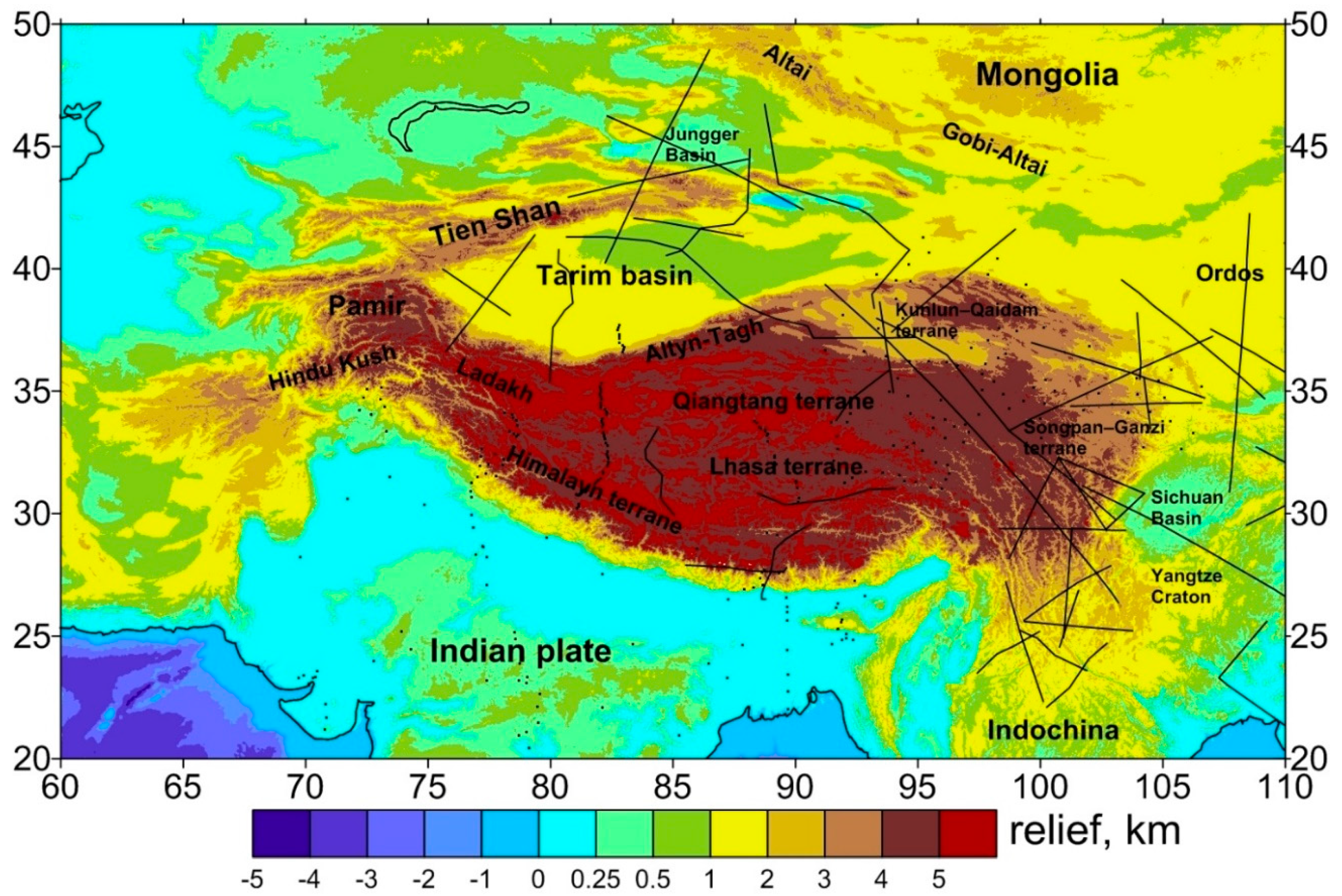
The gravity data analysis was conducted within the study area bounded by parallels 20 and 50 arc-deg of the northern latitude and meridians 60 and 110 arc-deg of the eastern longitude. It is noted that the seismic analysis was restricted by the availability of data (see Figure 1). The most prominent tectonic feature in this study area is an active continent-to-continent collision of the Indian plate with the Tibetan block, responsible for the uplift of the Himalayas. Tomographic evidence also suggests the southward subduction of the Eurasian lithosphere beneath the Tibetan block. A significant compressional tectonism due to these processes resulted in the uplift of the whole Tibetan Plateau. Major geological provinces include also continental basins (Indo-Ganges, Qaidam, Tarim, Sichuan) and orogens (Hindu Kush, Tien Shan). The geological setting of the study area is shown in Figure 1.
2.2. Seismic Data
For the Bengal lowland and the Shillong Plateau in the east of the Indian peninsula, we used receiver functions data from [37,38] and data from P and S waves prepared by [39]. According to these studies, the Moho depth under the Bengal lowland is 38–40 km, while it deepens to 48–50 km towards the collision zone between the Indian tectonic plate and the Tibetan block. For the western part of India, we used the receiver functions data from [40], showing that the Moho depth there is mostly within 36–44 km. For the central part of the Indian tectonic plate, we used the receiver functions data from [41,42,43,44,45]. The analysis of these data revealed a relatively complex Moho geometry with depths within a wide range from 35–48 km in the central part, deepening to 40–44 km towards north, and reaching 50–58 km at the beginning of the collision zone. Across the collision zone characterized also by a rising topography, the Moho deepens from 46 km to 56–58 km according to the analysis of receiver functions data from [5]. In Ladakh, Moho locally deepens to ~80 km [46]. To the east, Moho deepens from 38 km for the Indian plate to 44–48 km under the Himalayan foothills [47]. The receiver functions data from [47] also revealed that further north, Moho deepens under the greater Himalayas and southern Tibet to 65–70 km. Beneath the Lhasa terrane, Moho deepens locally to ~80 km. The analysis of receiver functions data from Pakistan also revealed a complex Moho geometry with depths ranging from 52 km in the Peshawar basin to 68–72 km in the higher Himalayas [47].
The seismic dataset for China comprises mainly the receiver functions data and the seismic profiles collected by [48,49,50,51]. Receiver functions calculated for data collected by the INDEPTH-IV seismic array [52] indicate an average Moho depth 65–70 km beneath north-eastern Tibet, 50–55 km for the Qaidam basin with an abrupt change (from 50–70 km) towards the Kunlun Mountains. The Moho topography detected from receiver functions data beneath western Tibet (ANTILOPE-1 profile) is rather uneven [53]. Moho there deepens from ~50 km to 75–78 km under margins of the Himalayas and then shallowing to 66–70 km under the central Lhasa terrane. For the Qiangtang terrane, the Moho depth is typically ~70 km, but abruptly shallows to 43–45 km at the beginning of the Tarim basin. The deep seismic sounding profiles from [54] exposed a sharp Moho depth change from 60 km under the east Kunlun to 48–50 km under the Zaige basin. For the north-eastern margin of the Tibetan Plateau, the receiver functions data from the ASCENT project [55] exhibited large Moho undulations within the range of 40–60 km. In the Qinling-Qilian block, Moho becomes shallower gradually from the west to the east. To the east of 105° E, the average Moho depth is ~45 km, whereas it exceeds 50 km to the west. Seismic data from [56,57,58,59,60,61], comprising the receiver functions data at 252 stations and the deep seismic sounding profiles, provide a detailed Moho map covering a broad region of the eastern part of the Tibetan Plateau and including also the Sichuan basin, the Ordos block, and the Yangtze Craton. According to these data, the Moho depth decreases from the eastern margin of the Tibetan Plateau (68–72 km) to the southern part of Yangtze Craton (28–30 km) and the Ordos block (38–42 km). Other regions are characterized by a complex Moho topography with depths: 52–56 km for the Qilian orogen, 40–44 km for the Qinling-Dabie orogen, 50–54 km for the Songpan-Ganzi terrane, 40–44 km for the Sichuan basin, 48–52 km for the Chuandian Plateau, and 28–36 km for the Yangtze Craton. According to results obtained from processing the receiver functions data by [62], the Moho depth under the north-east part of the Tibetan Plateau is typically within 50–52 km. Beneath the Liupan Mountains, Moho deepens to 52–54 km. Moho in the south-western part of the Ordos block is typically ~50 km. To the south, the deep seismic sounding profiles from [63,64,65,66] indicate that Moho changes from 34–44 km.
2.3. Gravity Data
The isostatic gravity disturbances used in this study for a gravimetric Moho inversion were computed according to numerical steps, explained next.
2.3.1. Free-Air Gravity Data
The free-air gravity disturbances δgFA were computed from the EIGEN-6C4 [67] gravitational coefficients Tn,m corrected for the GRS80 (Geodetic Reference System 1980) [68] normal gravity component using the following expression [69]:
where GM is the geocentric gravitational constant, R is the Earth’s mean radius, Yn,m are the surface spherical functions of degree n and order m, and is the upper summation index of spherical harmonics. The 3D position in Equation (1) and thereafter is defined in the spherical coordinate system ; where r is the radius and is the spherical direction with the spherical latitude φ and longitude λ.
2.3.2. Bouguer Gravity Data
The Bouguer gravity disturbances δgB were obtained from the free-air gravity disturbances δgFA after applying the topographic gT and stripping gravity corrections due to density contrasts of the ocean (i.e., bathymetry) gB, the ice gI, sediments gS, and the consolidated crust gC. Hence, we write:
The gravity corrections applied in Equation (2) were computed using the following generalized expression [70,71,72]:
The potential coefficients Vn,m are defined by:
where is the Earth’s mean density, and the coefficients {} read:
The coefficients { } in Equation (5) describe the geometry and density (or density contrast) distribution within a particular volumetric mass density layer.
Topographic and stripping gravity corrections due to the bathymetry and the ice were computed using the Earth2014 datasets [73]. A depth-dependent seawater density model was adopted in the definition of the ocean density contrast. For the reference crustal density of 2900 kg m−3 and the surface seawater density of 1027.91 kg m−3 [74], the nominal ocean density contrast (at zero depth) equals 1872.09 kg m−3. The depth-density parameters (up to the second-order density term) were given in [75,76]. The glacial density of 917 kg m−3 [77] was adopted to compute the ice-stripping gravity correction. The stripping gravity corrections attributed to sediments and the consolidated crust were computed from the CRUST1.0 global seismic crustal model [78]. It is noted that the atmospheric gravity correction is completely negligible in the context of the gravimetric Moho modelling, having maxima less than 1 mGal [79].
2.3.3. Isostatic Gravity Data
Finally, the isostatic gravity disturbances δgI were computed from the Bouguer gravity disturbances δgB by applying the compensation attraction gVMM, so that:
The compensation attraction gVMM in Equation (6) reads [34]:
where G is the Newton’s gravitational constant, Δρc/m is the Moho density contrast, and the values of the Moho depth D were used from a new seismic model (Section 3.1).
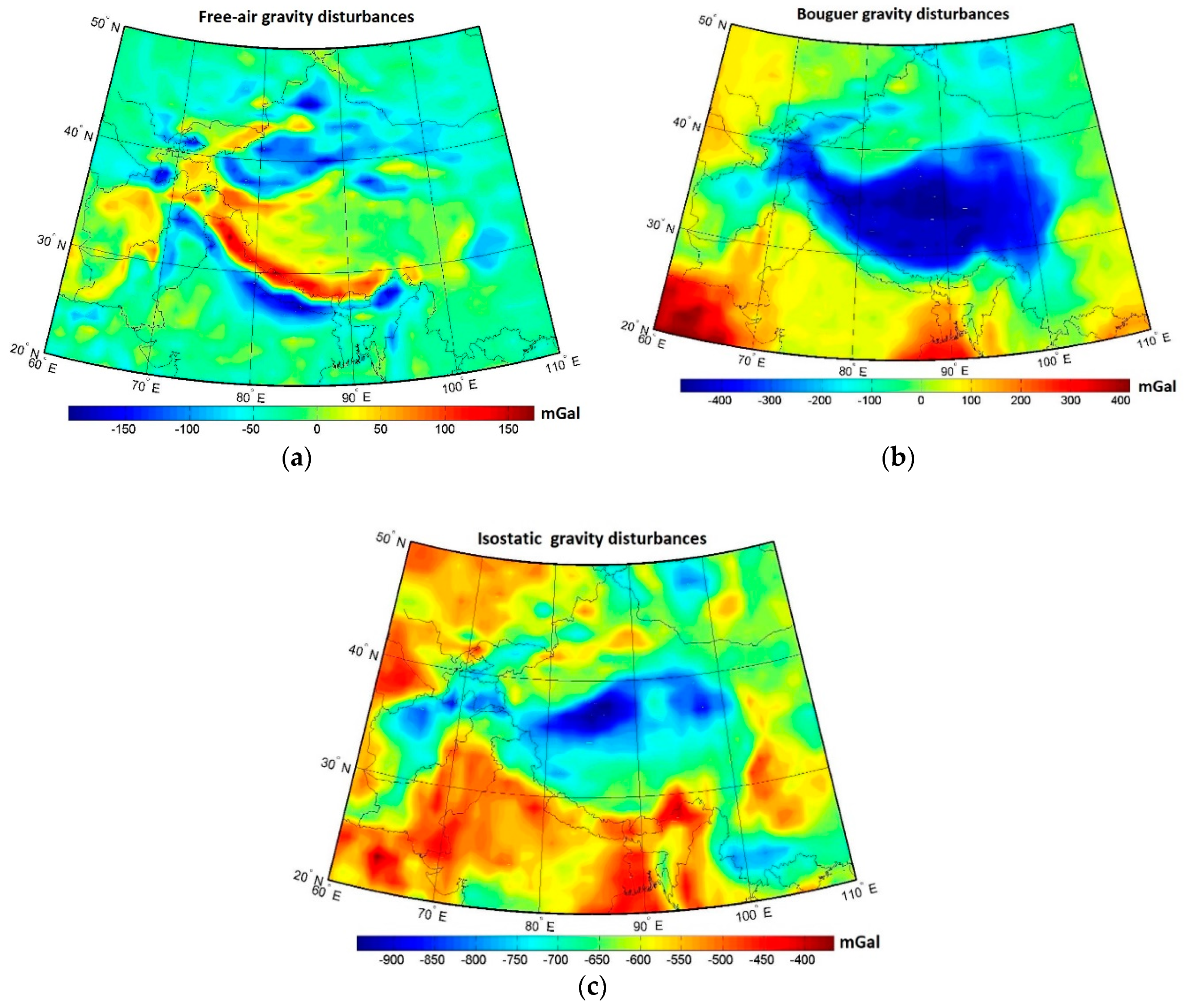
2.4. Gravity Maps
Regional maps of the free-air, Bouguer, and isostatic gravity disturbances are shown in Figure 2 (for statistics, see Table 1). All gravity computations were realized on a 1 × 1 arc-deg grid with a spectral resolution complete to the spherical harmonic degree of 180. Values of the free-air gravity disturbances were mostly within ±50 mGal, except for gravity highs over the Himalayas, Tien Shan, and Hindu Kush. Gravity lows were along the Indo-Ganges basin (Figure 2a). Negative values of the free-air gravity disturbances also prevailed over the Tarim, Qaidam, and Sichuan basins. The Bouguer gravity map reveals the isostatic signature of major orogens, marked by large negative values (Figure 2b). The isostatic gravity disturbances were everywhere negative, indicating a systematic bias mainly due to unmolded mantle density heterogeneities (Figure 2c).
3. Method
The methodology applied to compute the seismic and gravimetric Moho models and their combination is described in this section.
3.1. Seismic Moho Model
We used the seismic data to compile the Moho model by applying a processing strategy similar to that used for the construction of recent continental-scale crustal models, for instance, by [31]. For this purpose, we first inspected the quality of seismic data and then used them to generate the Moho contours by applying a standard kriging technique. This method was chosen from among others as a widely-applied geo-statistical technique. The idea behind this geo-statistical method is to reproduce trends that were estimated from combining the seismic data and the relief. The kriging parameters were chosen as follows: the interpolation area was 60°–110° E, 20°–50° N, grid step 1 degree, no anisotropy, with a linear variogram, while setting a scale factor equal to one. The linear variogram was intended to find a local vicinity of the observed point and for weighting the observed points used in the function interpolation at a given grid point.
3.2. Isostatic Moho Model
We used isostatic gravity disturbances δgI (Figure 2c) to determine the Moho depth by solving the VMM inverse problem of isostasy defined in the following generic form [35]:
where dσ is the surface integration element and σ is the solid angle. The kernel K in Equation (8) is a function of the spherical angle ψ, and the parameter s = 1 − D/R is a function of the Moho depth D. Its spectral form reads:
where the Legendre polynomials Pn are defined for the argument t = cos ψ.
The expression in Equation (8) is the (non-linear) Fredholm integral equation of the first kind. Its direct solution (up to a second-order term) was derived in the following form [34]:
The Moho term D1 in Equation (10) was computed from the isostatic gravity coefficients as follows:
The singularity for ψ → 0 in the third constituent on the right-hand side of Equation (10) was solved by applying the surface integration over the inner zone [34].
3.3. Combined Moho Model
We applied the method of [36] to constrain the gravimetric solution by seismic data. The principle of this method is to compute the non-isostatic gravity correction in order to account for differences between the gravimetric and seismic models. The non-isostatic gravity correction was then applied to the isostatic gravity disturbances. The resulting isostatic gravity disturbances obtained after applying the non-isostatic correction were then used to compute the combined Moho model according to the VMM isostatic model (Equations (10) and (11)).
4. Results
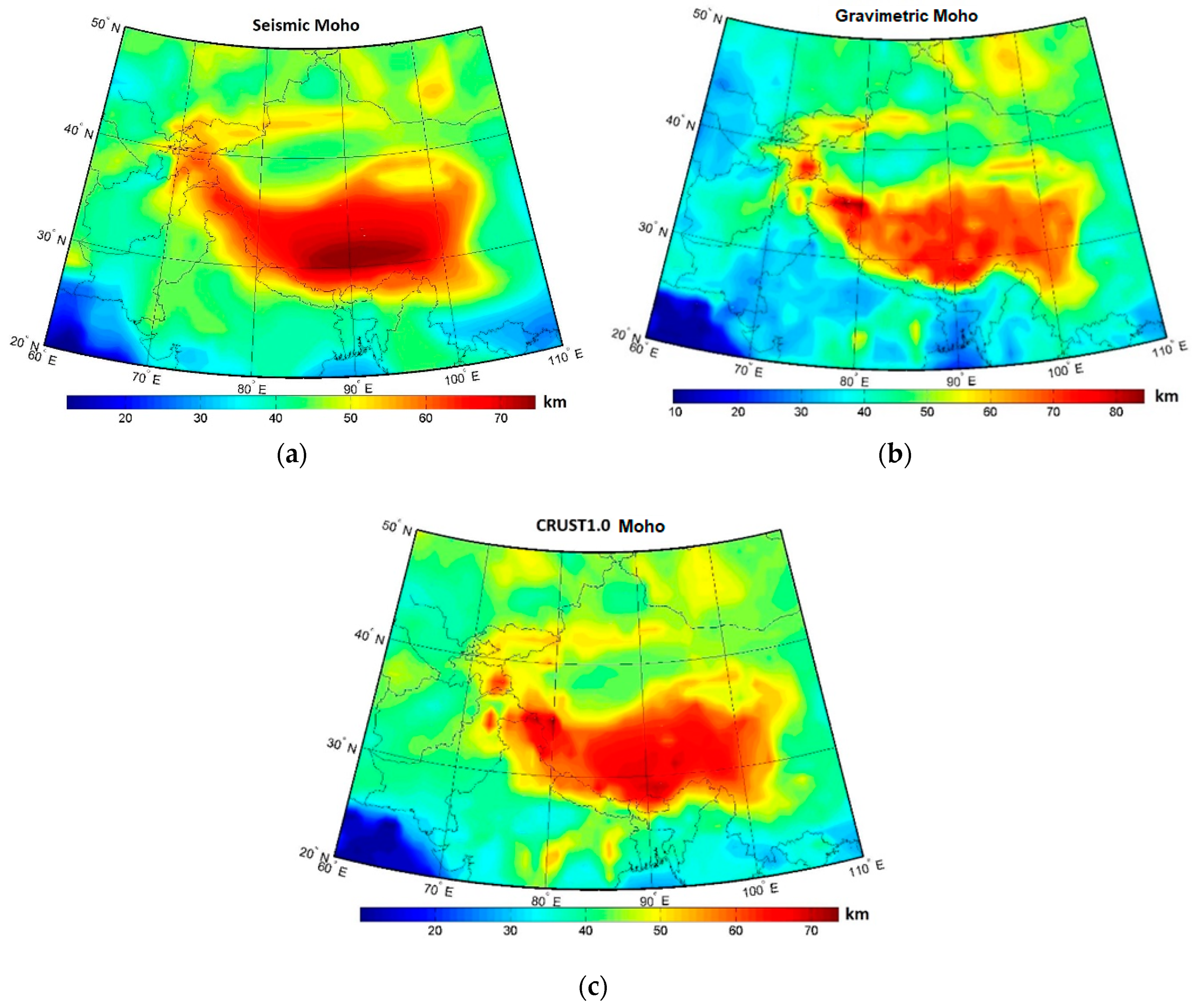
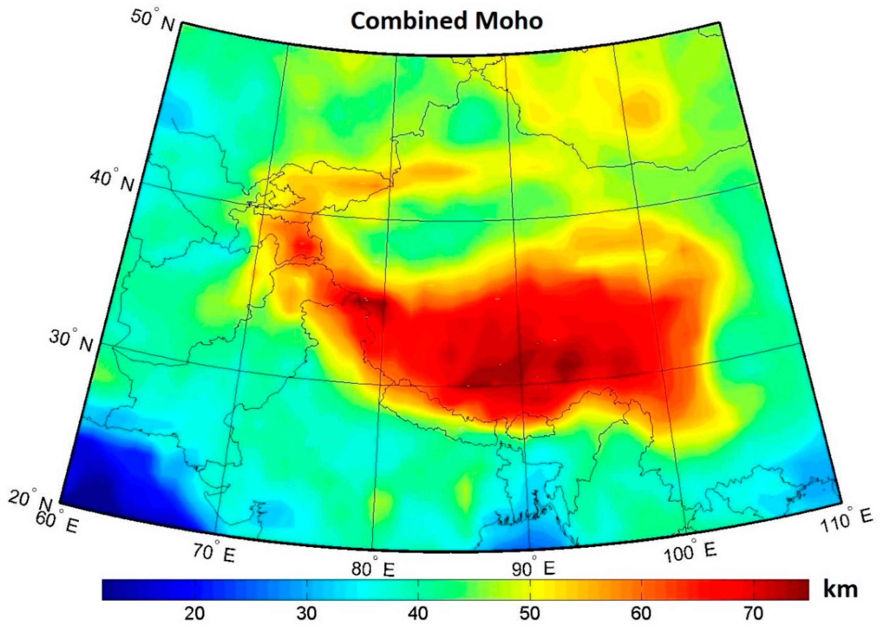
The seismic and gravimetric Moho models are shown in Figure 3 (for statistics, see Table 2). For the comparison, we also plotted the CRUST1.0 model. The final combined gravimetric-seismic Moho model is presented in Figure 4. Moho depth differences are plotted in Figure 5 (with the statistical summary given in Table 3).
The seismic Moho model (Figure 3a) exhibited a relatively smooth spatial pattern, partially due to the interpolation on a regular grid in areas where seismic data were sparse or missing. The Moho depth under the Indo-Ganges basin was mostly within 40–50 km. A similar Moho depth was found under the Tarim and Sichaun basins. The Moho depth in the Quadam basin exceeded 50 km. Major geological margins between orogens and basins were well pronounced with a significant Moho deepening under orogens. The orogenic belt of the Himalayas, Tibet, and Hindu Kush was characterized by a Moho depth exceeding 60 km and reaching the maximum depth of almost 76 km in the south and central Tibetan Plateau. This deep Moho extended eastwards under the western parts of the Hengduan Mountains. In contrast, the Tien Shan orogen was only slightly pronounced with the Moho depth reaching 52–56 km. The gravimetric Moho model (Figure 3b) revealed a more complex spatial pattern. Again, we could recognize a different crustal thickness of orogens and continental basins, but in this case, margins between geological provinces were much less pronounced in the Moho geometry. According to the VMM isostatic model applied in this study, the maximum Moho depending of ~86 km was detected under the Hindu Kush. Similarly, the maximum Moho deepening occurred there according to the CRUST1.0 seismic model (Figure 3c), but in this case to only ~75 km. The significant CRUST1.0 Moho deepening was also detected in parts of the south and central Tibetan Plateau.
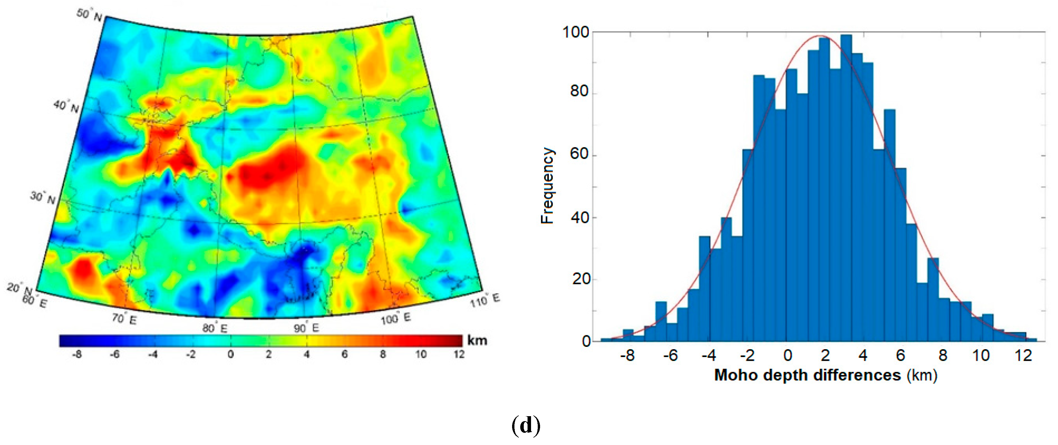
Compared to the seismic and gravimetric models (Figure 3a,b), the contrast between orogens and basins was much more pronounced in the combined Moho model (Figure 4). According to this result, the Moho depth under most of the Himalayas and the Tibetan Plateau typically varied within 60–70 km. The maximum Moho deepening to ~76 km occurred to the south of the Bangong-Nujiang suture under the Lhasa terrane. The Moho under Taksha at the Karakoram fault deepened to more than 70 km. Beneath the Hindu Kush and Tien Shan, the Moho depth was mostly within 55–65 km. The Tarim, Sichuan, and Indo-Ganges basins were characterized by a normal Moho with a typical depth of 38–47 km. The Moho depth in the Quadam basin slightly exceeded 50 km.
Comparison of Results
Despite overall similarities between the Moho solutions presented in Figure 3 and Figure 4, large localized differences existed (see Figure 5). As already stated, the seismic Moho model (Figure 3a) was relatively smooth with a maximum Moho deepening under the Lhasa terrane. The gravimetric Moho model (Figure 3b) exhibited a more complex Moho geometry, with a maximum deepening under the Karakoram fault. The combined Moho model (Figure 4) showed maxima of the Moho depth at both locations.
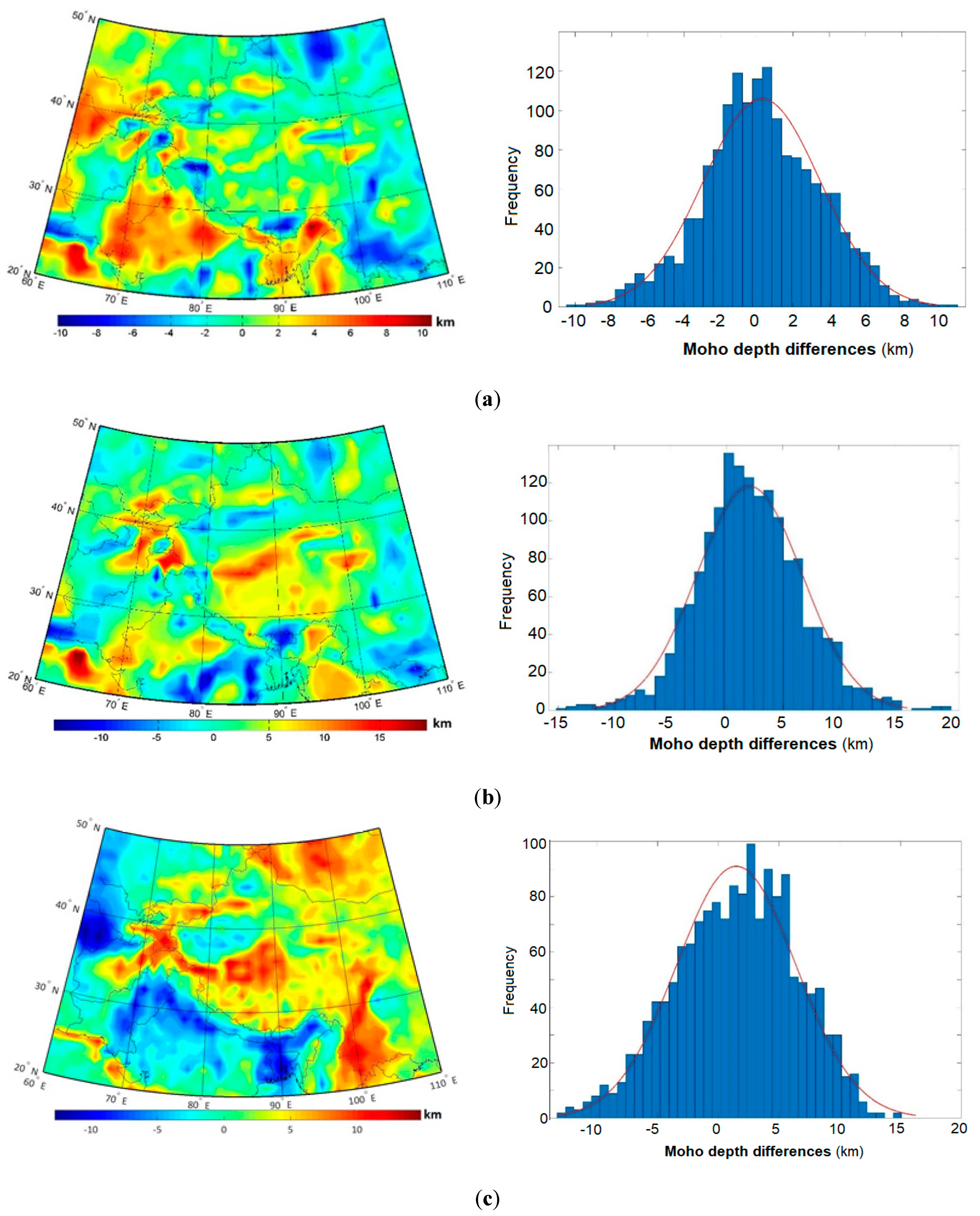
The interpolation of the Moho geometry in regions with a sparse seismic data coverage by using the gravity information modified the Moho solution only slightly within ±2 km for most of Tibet (Figure 5a). The corresponding modifications of the Moho geometry up to 8 km were, however, seen in the western and eastern parts of the Himalayas. Interestingly, the combined Moho model had a slightly better RMS fit with the CRUST1.0 than our gravimetric and seismic models (cf. Table 3).
5. Discussion
Our result based on the combined processing of gravity and seismic data (see Figure 4) revealed that the maximum Moho deepening of ~76 km occurred to the south of the Bangong-Nujiang suture under the Lhasa terrane. Deep Moho (~74 km) was also detected under Taksha at the Karakoram fault. This finding closely agrees with the results from teleseismic receiver function analysis of seismograms recorded on a ~700 km-long profile of 17 broadband seismographs traversing the north-west Himalayas conducted by [5]. They reported a progressive northward Moho deepening from ~40 km beneath Delhi south of the Himalayan foredeep to ~75 km beneath Taksha at the Karakoram fault. They also proposed that the Indian lithosphere might penetrate as far as the Bangong-Nujiang suture and possibly as far north as the Altyn Tagh. Alternative theories facilitated the hypothesis of crustal shortening and consequent crustal thickening attributed to the extrusion or escape tectonics mechanism [80]). According to these theories, the motion of the Indian plate pressed the Indochina block, and a proposed mechanism is that a large part of the crustal shortening was accommodated by thrusting and folding of the sediments of the passive Indian margin together with the deformation of the Tibetan crust [81].
A Moho depth largely between 60–70 km beneath most of the Himalayas and Tibet was reported in [7]. These values closely agree with our findings. Their result, however, indicated that the maximum Moho deepening of ~79 km occurred in the northern Tibet and the Himalayas. A maximum Moho deepening in northern Tibet along margins with the Tarim basin was also reported by [18]. According to their estimates, the Moho was more than 65 km deep under most of Tibet with maxima of ~82 km in its western part. A different Moho topography was presented by [21]. According to their result, the Moho depth in the west was deeper than that in the east, and the deepest Moho of ~77 km occurred beneath the western Qiangtang block. They also identified a Moho offset of approximately 5 km beneath the Yarlung-Zangbo suture at the juncture between the Himalayan and Lhasa blocks. Our combined Moho model also differed from the result presented by [14]. According to their result, the Moho depth under most of Tibet was largely within 70–75 km with the maximum deepening to ~80 km along margins of the plateau and a shallower depth of 65 km under the Bangong-Nujiang suture in central Tibet.
Accuracy Assessment
As follows from the discussion in the preceding paragraph, large inconsistencies exist between Moho models. Despite the assessment of accuracy of these models being generally not simple, two principal factors should be taken into consideration in this respect. These involve the quality of seismic and gravity data, as well as available information about the crustal density structure.
The best horizontal Moho resolution is typically inferred from reflection profiles [82], but such a technique is expensive, thus not widely used. The Moho detection from a two-way travel time might also be affected by a weak reflectivity. An intermediate spatial resolution could be obtained from a deep seismic sounding based on using refracted and wide-angle reflected waves. Uncertainties of detecting the Moho depth from the wide-angle reflection and refraction methods are typically 1–2 km. Another technique, which has become quite common during the last two decades, is based on inverting the P- or S-wave receiver functions [83,84]. The estimated uncertainty of this method is about 3 km. Intermediate-period surface waves are quite sensitive to crustal thickness, but are not able to discriminate it from the mantle velocity structure, thus they cannot be inverted uniquely [85,86].
To interpolate the Moho information over regions where seismic data are sparse or missing, we used the gravity data and information about the crustal density structure. Moho depth uncertainties attributed to errors in gravity data are relatively small, because the accuracy of the latest global gravitational models of about ±10 mGal or better is expected globally at a resolution of about 100 km [87,88]. Errors in topographic models are completely negligible in the context of a gravimetric Moho recovery. However, relative errors in the estimated Moho depth of 10% or more could be expected due to uncertainties within the CRUST1.0 sediment and consolidated crustal density layers [31].
6. Conclusions
We have used seismic, gravity, and topographic data to estimate the Moho depth of the orogenic formations of the Himalayas, Tibet, Hindu Kush, and Tien Shan, including also the surrounding continental basins of Indo-Ganges, Tarim, Sichaun, and Quadam. According to our combined gravimetric-seismic model, the Moho depth under the Himalayas and the Tibetan Plateau is mostly within 60–70 km. The maximum Moho deepening of ~76 km occurs to the south of the Bangong-Nujiang suture under the Lhasa terrane. The additional significant Moho deepening to ~74 km was detected beneath Taksha at the Karakoram fault. A large Moho depth of 60–65 km was also confirmed beneath the Hindu Kush and Tien Shan. In contrast to a large continental crustal thickness of these orogenic formations, the Tarim, Sichuan, and Indo-Ganges basins are characterized by a Moho depth typically within 38–47 km. Moho in the Quadam basin slightly exceeds the depth of 50 km. The mean Moho depth within the whole study area is estimated to be 46.5 km.
Reviewing seismic and gravimetric studies, we identified some significant discrepancies between existing Moho models of Tibet. Based on our assumptions, we expect that errors in estimated values of the Moho depth from the seismic data analysis are typically less than 5 km, but could reach as much as 10–15 km when interpolated using the gravity information. These large errors are mainly due to the fact that a Moho recovery from the gravity data requires the knowledge of crustal density structure. The accuracy of currently available global and regional crustal/lithospheric models is obviously restricted, with expected relative uncertainties of 10% or more, especially in geologically-complex regions. Another problem is that isostatic theories could not realistically reproduce a Moho geometry, especially along active tectonic margins. All these factors obviously affect the accuracy of the combined Moho model.
Author Contributions
A.B. and M.B. performed the numerical studies and validations; R.T. analyzed the results and compiled the manuscript.
Funding
This research was funded by the Hong Kong Research Grants Council, Project 1-ZE8F: Remote-sensing data for studying the Earth’s and planetary inner structure, and the Russian Foundation for Basic Research, grant: 16-55-12033.
Conflicts of Interest
The authors declare no conflict of interest. The founding sponsors had no role in the design of the study; in the collection, analyses, or interpretation of data; in the writing of the manuscript; nor in the decision to publish the results.
References
- Teng, J.W.; Yin, Z.X.; Wnag, X.T.; Lu, D.Y. Structure of the crust and upper mantle pattern and velocity distributional characteristics in the Northern Himalayan mountain region. Acta Geophys. Sin. 1983, 26, 525–540. [Google Scholar] [CrossRef]
- Tilmann, F.; Ni, J.; INDEPTH III Seismic Team. Seismic imaging of the downwelling Indian lithosphere beneath central Tibet. Science 2003, 300, 1424–1427. [Google Scholar] [CrossRef]
- Allègre, C.J.; Courtillot, V.; Tapponnier, P.A.; Hirn, M.; Mattauer, C.; Coulon, J.J.; Jaeger, J.; Achache, U.; Schärer, J.; Marcoux, J.P.; et al. Structure and evolution of the Himalaya-Tibet orogenic belt. Nature 1984, 307, 17–22. [Google Scholar] [CrossRef]
- Zhao, W.; Nelson, K.D.; Che, J.; Quo, J.; Lu, D.; Wu, C.; Liu, X. Deep seismic reflection evidence for continental underthrusting beneath southern Tibet. Nature 1993, 366, 557–559. [Google Scholar] [CrossRef]
- Rai, S.S.; Priestley, K.; Gaur, V.K.; Mitra, S.; Singh, M.P.; Searle, M. Configuration of the Indian Moho beneath the NW Himalaya and Ladakh. Geophys. Res. Lett. 2006, 33, L15308. [Google Scholar] [CrossRef]
- Wittlinger, G.; Vergne, J.; Tapponnier, P.; Farra, V.; Poupinet, G.; Jiang, M.; Su, H.; Herquel, G.; Paul, A. Teleseismic imaging of subducting lithosphere and Moho offsets beneath western Tibet. Earth Planet. Sci. Lett. 2004, 221, 117–130. [Google Scholar] [CrossRef]
- Tenzer, R.; Bagherbandi, M.; Hwang, C.H.; Chang, E.T.Y. Moho interface modeling beneath Himalayas, Tibet and central Siberia using GOCO02S and DTM2006.0. Special issue on geophysical and climate change studies in Tibet, Xinjiang, and Siberia from satellite geodesy. Terr. Atm. Ocean. Sci. 2013, 24, 581–590. [Google Scholar] [CrossRef]
- Reigber, C.; Bock, R.; Forste, C.; Grunwaldt, L.; Jakowski, N.; Lühr, H.; Schwintzer, P.; Tilgner, C. CHAMP Phase-B Executive Summary; STR96/13; G.F.Z.: Potsdam, Germany, 1996. [Google Scholar]
- Reigber, C.; Schwintzer, P.; Lühr, H. The CHAMP geopotential mission. Boll. Geofis. Teor. Appl. 1999, 40, 285–289. [Google Scholar]
- Reigber, C.; Lühr, H.; Schwintzer, P. CHAMP mission status. Adv. Space Res. 2002, 30, 129–134. [Google Scholar] [CrossRef]
- Tapley, B.D.; Bettadpur, S.; Watkins, M.; Reigber, C. The gravity recovery and climate experiment: Mission overview and early results. Geophys. Res. Lett. 2004, 31, L09607. [Google Scholar] [CrossRef]
- Drinkwater, M.R.; Floberghagen, R.; Haagmans, R.; Muzi, D.; Popescu, A. GOCE: ESA’s First Earth Explorer Core Mission. In Earth Gravity Field from Space-From Sensors to Earth Science; Beutler, G., Ed.; Kluwer Academic: Dordrecht, The Netherlands, 2003; Volume 18, pp. 419–432. [Google Scholar]
- Floberghagen, R.; Fehringer, M.; Lamarre, D.; Muzi, D.; Frommknecht, B.; Steiger, C.; Piñeiro, J.; da Costa, A. Mission design, operation and exploitation of the gravity field and steady-state ocean circulation explorer mission. J. Geod. 2011, 85, 749–758. [Google Scholar] [CrossRef]
- Braitenberg, C.; Zadro, M.; Fang, J.; Wang, Y.; Hsu, H.T. The gravity and isostatic Moho undulations in Qinghai-Tibet plateau. J. Geodyn. 2000, 30, 489–505. [Google Scholar] [CrossRef]
- Braitenberg, C.; Pettenati, F.; Zadro, M. Spectral and classical methods in the evaluation of Moho undulations from gravity data: The N-E Italian Alps and isostasy. J. Geodyn. 1997, 23, 5–22. [Google Scholar] [CrossRef]
- Braitenberg, C.; Drigo, R. A crustal model from gravity inversion in Karakorum. In Proceedings of the International Symposium on Current Crustal Movement and Hazard Reduction in East Asia and Soth-East Asia, Wuhan, China, 4–7 November 1997; pp. 325–341. [Google Scholar]
- Caporali, A. Buckling of the lithosphere in western Himalaya: Constraints from gravity and topography data. J. Geophys. Res. 2000, 105, 3103–3113. [Google Scholar] [CrossRef] [Green Version]
- Shin, Y.H.; Shum, C.K.; Braitenberg, C.; Lee, S.M.; Na, S.-H.; Choi, K.S.; Hsu, H.; Park, Y.-S.; Lim, M. Moho topography, ranges and folds of Tibet by analysis of global gravity models and GOCE data. Sci. Rep. 2015, 5, 11681. [Google Scholar] [CrossRef] [Green Version]
- Tenzer, R.; Bagherbandi, M.; Sjöberg, L.E.; Novák, P. Isostatic crustal thickness under the Tibetan Plateau and Himalayas from satellite gravity gradiometry data. Earth Sci. Res. J. 2015, 19, 97–106. [Google Scholar] [CrossRef]
- Tenzer, R.; Chen, W. Regional gravity inversion of crustal thickness beneath the Tibetan plateau. Earth Sci. Inform. 2014, 7, 265–276. [Google Scholar] [CrossRef]
- Xu, C.; Liu, Z.; Luo, Z.; Wu, Y.; Wang, H. Moho topography of the Tibetan Plateau using multiscale gravity analysis and its tectonic implications. J. Asian Earth Sci. 2017, 138, 378–386. [Google Scholar] [CrossRef]
- Parker, R.L. The rapid calculation of potential anomalies. Geophys. J. R. Astr. Soc. 1972, 31, 447–455. [Google Scholar] [CrossRef]
- Oldenburg, D.W. The inversion and interpretation of gravity anomalies. Geophysics 1974, 39, 526–536. [Google Scholar] [CrossRef]
- Tenzer, R.; Vajda, P. A global correlation of the step-wise consolidated crust-stripped gravity field quantities with the topography, bathymetry, and the CRUST 2.0 Moho boundary. Contr. Geophys. Geod. 2009, 39, 133–147. [Google Scholar] [CrossRef] [Green Version]
- Tenzer, R.; Bagherbandi, M. Theoretical deficiencies of isostatic schemes in modelling the crustal thickness along the convergent continental tectonic plate boundaries. J. Earth Sci. 2016, 27, 1045–1053. [Google Scholar] [CrossRef]
- Tenzer, R.; Chen, W.; Jin, S. Effect of the upper mantle density structure on the Moho geometry. Pure App. Geophys. 2015, 172, 1563–1583. [Google Scholar] [CrossRef]
- Zhang, Z.; Li, Y.; Wang, G.; Teng, J.; Klemperer, S.; Li, J.; Fan, J.; Chen, Y. East-west crustal structure and “down-bowing” Moho under the northern Tibet revealed by wide-angle seismic profile. Sci. Chin. Ser. D Earth Sci. 2002, 45, 550–558. [Google Scholar] [CrossRef]
- Li, X.; Wei, D.; Yuan, X.; Kind, R.; Kumar, P.; Zhou, H. Details of the doublet Moho structure beneath Lhasa, Tibet, obtained by comparison of P and S receiver functions. Bull. Seismol. Soc. Am. 2011, 101, 1259–1269. [Google Scholar] [CrossRef]
- Zhang, Z.; Wang, Y.; Houseman, G.A.; Xu, T.; Wu, Z.; Yuan, X.; Chen, Y.; Tian, X.; Bai, Z.; Teng, J. The Moho beneath western Tibet: Shear zones and eclogitization in the lower crust. Earth Planet. Sci. Lett. 2014, 408, 370–377. [Google Scholar] [CrossRef]
- Teng, J.; Zhang, Z.; Zhang, X.; Wang, C.; Gao, R.; Yang, B.; Qiao, Y.; Deng, Y. Investigation of the Moho discontinuity beneath the Chinese mainland using deep seismic sounding profiles. Tectonophysics 2013, 609, 202–216. [Google Scholar] [CrossRef]
- Baranov, A.; Tenzer, R.; Bagherbandi, M. Combined gravimetric-seismic crustal model for Antarctica. Surv. Geophys. 2018, 39, 23–56. [Google Scholar] [CrossRef]
- Vening Meinesz, F.A. Une nouvelle méthode pour la réduction isostatique régionale de Í intensité de la pesanteur. Bull. Geod. 1931, 29, 33–51. [Google Scholar] [CrossRef]
- Moritz, H. The Figure of the Earth; Wichmann: Karlsruhe, Germany, 1990. [Google Scholar]
- Sjöberg, L.E. Solving Vening Meinesz-Moritz inverse problem in isostasy. Geophys. J. Int. 2009, 179, 1527–1536. [Google Scholar] [CrossRef] [Green Version]
- Sjöberg, L.E. On the isostatic gravity anomaly and disturbance and their applications to Vening Meinesz-Moritz inverse problem of isostasy. Geophys. J. Int. 2013, 193, 1277–1282. [Google Scholar] [CrossRef]
- Sjöberg, L.E.; Bagherbandi, M. A method of estimating the Moho density contrast with a tentative application by EGM08 and CRUST2.0. Acta Geophys. 2011, 58, 1–24. [Google Scholar] [CrossRef]
- Mitra, S.; Priestley, K.; Bhattacharyya, A.; Gaur, V. Crustal Structure and Earthquake Focal Depths Beneath Norteastern India and Southern Tibet. Geophys. J. Int. 2005, 160, 227–248. [Google Scholar] [CrossRef]
- Mitra, S.; Bhattacharya, S.N.; Nath, S.K. Crustal structure of the Western Bengal Basin from joint analysis of teleseismic receiver functions and Rayleigh wave dispersion. Bull. Seismol. Soc. Am. 2008, 98, 2715–2723. [Google Scholar] [CrossRef]
- Maggi, A.; Jackson, J.; Priestley, K.; Baker, C. A Reassessment of Focal Depth Distributions in Southern Iran, the Tien Shan and Northern India: Do Earthquakes Really Occur in the Continental Mantle? Geophys. J. Int. 2000, 143, 629–661. [Google Scholar] [CrossRef]
- Mandal, P. Sedimentary and Crustal Structure Beneath Kachchh and Saurashtra Regions, Gujarat, India. Phys. Earth Planet. Int. 2006, 155, 286–299. [Google Scholar] [CrossRef]
- Kumar, R.; Saul, J.; Sarkar, D.; Kind, R.; Shulda, A. Crustal Structure of the Indian Shield: New Constraints from teleseismic receiver functions. Geophys. Res. Lett. 2001, 28, 1339. [Google Scholar] [CrossRef]
- Priestley, K.; Jackson, J.; McKenzie, D. Lithospheric Structure and Deep Earthquakes Beneath India, the Himalaya and Southern Tibet. Geophys. J. Int. 2008, 172, 345–362. [Google Scholar] [CrossRef]
- Saikia, C. Modeling of the 21 May 1997 Jabalpur Earthquake in Central India: Source Parameters and Regional Path Calibration. Bull. Seismol. Soc. Am. 2006, 96, 1396–1421. [Google Scholar] [CrossRef]
- Jagadeesh, J.; Rai, S. Thickness, composition, and evolution of the Indian Precambrian crust inferred from broadband seismological measurements. Precambrian Res. 2008, 162, 4–15. [Google Scholar] [CrossRef]
- Kayal, J.R.; Srivastava, V.K.; Kumar, P.; Chatterjee, R.; Khan, P.K. Evaluation of crustal and upper mantle structures using receiver function analysis: ISM broadband observatory data. J. Geol. Soc. India 2011, 78, 76–80. [Google Scholar] [CrossRef]
- Acton, C.E.; Priestley, K.; Mitra, S.; Gaur, V.K. Crustal structure of the Darjeeling–Sikkim Himalaya and Southern Tibet. Geophys. J. Int. 2011, 184, 829–852. [Google Scholar] [CrossRef]
- Li, A.; Mashele, B. Crustal structure in the Pakistan Himalaya from teleseismic receiver functions. Geochem. Geophys. Geosyst. 2009, 10, Q12010. [Google Scholar] [CrossRef]
- Li, Y.; Gao, M.; Wu, Q. Crustal thickness map of the Chinese mainland from teleseismic receiver functions. Tectonophysics 2014, 611, 51–60. [Google Scholar] [CrossRef]
- Baranov, A. A new crustal model for Central and Southern Asia. Izvest. Phys. Solid Earth 2010, 46, 34–46. [Google Scholar] [CrossRef]
- Li, S.; Mooney, W.; Fan, J. Crustal Structure of Mainland China from Deep Seismic Sounding Data. Tectonophysics 2006, 420, 239–252. [Google Scholar] [CrossRef]
- He, R.; Shang, X.; Yu, CH.; Zhang, H.; Van der Hilst, R. A unified map of Moho depth and Vp/Vs ratio of continental China by receiver function analysis. Geophys. J. Int. 2014, 199, 1910–1918. [Google Scholar] [CrossRef]
- Yue, H.; Chen, Y.J.; Sandvol, E.; Ni, J.; Hearn, T.; Zhou, S.; Feng, Y.; Ge, Z.; Trujillo, A.; Wang, Y.; Jin, G. Lithospheric and upper mantle structure of the northeastern Tibetan Plateau. J. Geophys. Res. 2012, 117, B05307. [Google Scholar] [CrossRef]
- Murodov, D.; Zhao, J.; Xu, Q.; Liu, H.; Pei, S. Complex N–S variations in Moho depth and Vp/Vs ratio beneath the western Tibetan Plateau as revealed by receiver function analysis. Geophys. J. Int. 2018, 214, 895–906. [Google Scholar] [CrossRef]
- Jia, S.; Zhang, X.; Zhao, J.; Wang, F.; Zhang, C.; Xu, Z.; Pan, J.; Liu, Z.; Pan, S.; Sun, G. Deep seismic sounding data reveal the crustal structures beneath Zoigê basin and its surrounding folded orogenic belts. Sci China Earth Sci. 2010, 53, 203–212. [Google Scholar] [CrossRef]
- Liu, Q.M.; Zhao, J.M.; Lu, F.; Liu, H. Crustal structure of northeastern margin of the Tibetan Plateau by receiver function inversion. Sci China Earth Sci. 2014, 57, 741. [Google Scholar] [CrossRef]
- Xu, X.M.; Ding, Z.F.; Shi, D.N.; Li, X.F. Receiver function analysis of crustal structure beneath the eastern Tibetan plateau. J. Asian Earth Sci. 2013, 73, 121–127. [Google Scholar] [CrossRef]
- Wang, C.Y.; Han, W.B.; Wu, J.P.; Lou, H.; Chan, W.W. Crustal structure beneath the eastern margin of the Tibetan Plateau and its tectonic implications. J. Geophys. Res. 2007, 112, B07307. [Google Scholar] [CrossRef]
- Xu, X.; Li, H.Y.; Gong, M.; Ding, Z.F. Three-dimensional S-Wave velocity structure in eastern Tibet from ambient noise Rayleigh and love wave tomography. J. Earth Sci. 2011, 22, 195–204. [Google Scholar] [CrossRef]
- Zhang, Z.J.; Yuan, X.H.; Chen, Y.; Tian, X.B.; Kind, R.; Li, X.Q.; Teng, J.W. Seismic signature of the collision between the east Tibetan escape flow and the Sichuan Basin. Earth Planet. Sci. Lett. 2010, 292, 254–264. [Google Scholar] [CrossRef] [Green Version]
- Xu, L.; Rondenay, S.; van der Hilst, R.D. Structure of the crust beneath the southeastern Tibetan Plateau from teleseismic receiver functions. Phys. Earth Planet. Int. 2007, 165, 176–193. [Google Scholar] [CrossRef] [Green Version]
- Xu, Q.; Zhao, J.M.; Cui, Z.X.; Pei, S.P.; Liu, H.B. Moho offset beneath the central Bangong–Nujiang suture of Tibetan Plateau. Chin. Sci. Bull. 2010, 55, 607–613. [Google Scholar] [CrossRef]
- Tong, W.; Wang, L.; Mi, N.; Ming, H.; Li, H.; Yu, D.; Li, C.; Liu, S.; Liu, M.; Sandvol, E. Receiver function analysis for seismic structure of the crust and uppermost mantle in the Liupanshan area, China. Sci. Chin. Ser. D Earth Sci. 2007, 50, 227. [Google Scholar] [CrossRef]
- Gao, Z.; Zhao, Y.; Deng, X.; Yang, Y. Crustal structure along the Zhenkang–Luxi deep seismic sounding profile in Yunnan derived from receiver functions. Geod. Geodyn. 2018, 9, 334–341. [Google Scholar] [CrossRef]
- Yan, Q.; Zhang, G.; Kan, R.; Hu, H. The crustal structure of Simao to Malong profile, Yunnan province, China. J. Seism. Res. 1985, 8, 249–280. [Google Scholar]
- Wang, C.; Lou, H.; Wang, X.; Qin, J.; Yang, R.; Zhao, J. Crustal structure in Xiaojiang fault zone and its vicinity. Earth Sci. 2009, 22, 347–356. [Google Scholar] [CrossRef]
- Zhang, X.; Wang, Y. Crustal and upper mantle velocity structure in Yunnan, Southwest China. Tectonophysics 2009, 471, 171–185. [Google Scholar] [CrossRef] [Green Version]
- Förste, C.; Bruinsma, S.L.; Abrikosov, O.; Lemoine, J.-M.; Marty, J.C.; Flechtner, F.; Balmino, G.; Barthelmes, F.; Biancale, R. EIGEN-6C4—The Latest Combined Global Gravity Field Model Including GOCE Data up to Degree and Order 2190 of GFZ Potsdam and GRGS Toulouse; GFZ Data Services; Tapley, B.D., Bettadpur, S., Watkins, M., Eds.; GFZ German Research Centre for Geosciences: Potsdam, Germany, 2014. [Google Scholar]
- Moritz, H. Geodetic Reference System 1980. J. Geod. 2000, 74, 128–162. [Google Scholar] [CrossRef]
- Heiskanen, W.A.; Moritz, H. Physical Geodesy; W.H. Freeman and Co.: San Francisco, CA, USA; London, UK, 1967. [Google Scholar]
- Tenzer, R.; Vajda, P. Global maps of the CRUST2.0 components stripped gravity disturbances. J. Geophys. Res. 2009, 114, B05408. [Google Scholar] [CrossRef]
- Tenzer, R.; Gladkikh, V.; Vajda, P.; Novák, P. Spatial and spectral analysis of refined gravity data for modelling the crust-mantle interface and mantle-lithosphere structure. Surv. Geophys. 2012, 33, 817–839. [Google Scholar] [CrossRef]
- Tenzer, R.; Chen, W.; Tsoulis, D.; Bagherbandi, M.; Sjöberg, L.E.; Novák, P.; Jin, S. Analysis of the refined CRUST1.0 crustal model and its gravity field. Surv. Geophys. 2015, 36, 139–165. [Google Scholar] [CrossRef]
- Hirt, C.; Rexer, M. Earth2014: 1 arc-min shape, topography, bedrock and ice-sheet models—Available as gridded data and degree-10,800 spherical harmonics. Int. J. Appl. Earth Obs. Geoinf. 2015, 39, 103–112. [Google Scholar] [CrossRef]
- Gladkikh, V.; Tenzer, R. A mathematical model of the global ocean saltwater density distribution. Pure Appl. Geophys. 2011, 169, 249–257. [Google Scholar] [CrossRef]
- Tenzer, R.; Novák, P.; Gladkikh, V. The bathymetric stripping corrections to gravity field quantities for a depth-dependent model of the seawater density. Mar. Geod. 2012, 35, 198–220. [Google Scholar] [CrossRef]
- Tenzer, R.; Vajda, P.; Hamayun, P. A mathematical model of the bathymetry-generated external gravitational field. Contrib. Geophys. Geod. 2010, 40, 31–44. [Google Scholar] [CrossRef] [Green Version]
- Cutnell, J.D.; Kenneth, W.J. Physics, 3rd ed.; Wiley: New York, NY, USA, 1995. [Google Scholar]
- Laske, G.; Masters, G.; Ma, Z.; Pasyanos, M.E. Update on CRUST1.0—A 1-degree global model of Earth’s crust. Geophys. Res. Abstr. 2013, 15, 2658. [Google Scholar]
- Tenzer, R.; Vajda, P.; Hamayun, P. Global atmospheric corrections to the gravity field quantities. Contr. Geophys. Geod. 2009, 39, 221–236. [Google Scholar] [CrossRef]
- Molnar, P.; Tapponnier, P. Cenozoic tectonics of Asia: Effects of a continental collision. Science 1975, 189, 419–426. [Google Scholar] [CrossRef] [PubMed]
- Dewey, J.F.; Cande, S.; Pitman, W.C. Tectonic evolution of the Indian/Eurasia collision zone. Eclog. Geol. Helv. 1989, 82, 717–734. [Google Scholar]
- Kanao, M.; Fujiwara, A.; Miyamachi, H.; Toda, S.; Tomura, M.; Ito, K.; Ikawa, T. Reflection imaging of the crust and the lithospheric mantle in the Lützow–Holm Complex, Eastern Dronning Maud Land, Antarctica, derived from the SEAL Transects. Tectonophysics 2011, 508, 73–84. [Google Scholar] [CrossRef]
- Zhu, L.; Kanamori, H. Moho depth variation in Southern California from teleseismic receiver functions. J. Geophys. Res. 2000, 105, 2969–2980. [Google Scholar] [CrossRef]
- Hansen, S.; Nyblade, A.; Pyle, M.; Wiens, D.; Anandakrishnan, S. Using S wave receiver functions to estimate crustal structure beneath ice sheets: An application to the Transantarctic Mountains and East Antarctic craton. Geoch. Geophys. Geosyst. 2009, 10, Q08014. [Google Scholar] [CrossRef]
- Danesi, S.; Morelli, A. Structure of the upper mantle under the Antarctic Plate from surface wave tomography. Geophys. Res. Lett. 2001, 28, 4395–4398. [Google Scholar] [CrossRef] [Green Version]
- Ritzwoller, M.H.; Shapiro, N.M.; Levshin, A.L.; Leahy, G.M. Crustal and upper mantle structure beneath Antarctica and surrounding oceans. J. Geophys. Res. B 2001, 106, 30645–30670. [Google Scholar] [CrossRef] [Green Version]
- Pail, R.; Goiginger, H.; Schuh, W.-D.; Höck, E.; Brockmann, J.M.; Fecher, T.; Gruber, T.; Mayer-Gürr, T.; Kusche, J.; Jäggi, A.; et al. Combined satellite gravity field model GOCO01S derived from GOCE and GRACE. Geophys. Res. Lett. 2010, 37, L20314. [Google Scholar] [CrossRef]
- Pail, R.; Bruinsma, S.; Migliaccio, F.; Förste, C.; Goiginger, H.; Schuh, W.-D.; Höck, E.; Reguzzoni, M.; Brockmann, J.M.; Abrikosov, O.; et al. First GOCE gravity field models derived by three different approaches. J. Geod. 2011, 85, 819–843. [Google Scholar] [CrossRef] [Green Version]
Figure 1.
Geological setting of the study area. Black lines represent seismic profiles and black dots receiver functions.
Figure 1.
Geological setting of the study area. Black lines represent seismic profiles and black dots receiver functions.

Figure 2.
Regional gravity maps: (a) the free-air gravity disturbances, (b) the Bouguer gravity disturbances, and (c) the isostatic gravity disturbances.
Figure 2.
Regional gravity maps: (a) the free-air gravity disturbances, (b) the Bouguer gravity disturbances, and (c) the isostatic gravity disturbances.

Figure 3.
Moho models of Tibet: (a) seismic, (b) gravimetric, and (c) CRUST1.0.

Figure 4.
Combined gravimetric-seismic Moho model of Tibet.

Figure 5.
Moho depth differences: (a) seismic vs. combined, (b) seismic vs. CRUST1.0, (c) gravimetric vs. CRUST1.0, and (d) combined vs. CRUST1.0.
Figure 5.
Moho depth differences: (a) seismic vs. combined, (b) seismic vs. CRUST1.0, (c) gravimetric vs. CRUST1.0, and (d) combined vs. CRUST1.0.


Table 1.
Statistics of the free-air, Bouguer, and isostatic gravity disturbances.
| Gravity Disturbance | Min (mGal) | Max (mGal) | Mean (mGal) | STD (mGal) |
|---|---|---|---|---|
| Free-air | −195 | 177 | 23 | 45 |
| Bouguer | −483 | 436 | 54 | 185 |
| Isostatic | −945 | -353 | -614 | 94 |
Table 2.
Statistics of the Moho models.
| Moho Model | Min (km) | Max (km) | Mean (km) | STD (km) |
|---|---|---|---|---|
| Seismic | 8.0 | 75.8 | 31.1 | 13.9 |
| Gravimetric | 9.7 | 85.9 | 46.3 | 12.0 |
| Combined | 11.7 | 76.3 | 46.5 | 10.9 |
| CRUST1.0 | 10.0 | 74.8 | 44.7 | 9.8 |
Table 3.
Statistics of the regional Moho depth differences.
| Moho Differences | Min (km) | Max (km) | Mean (km) | RMS (km) |
|---|---|---|---|---|
| Seismic-Combined | −10.3 | 10.9 | 0.3 | 3.2 |
| Seismic-CRUST1.0 | −14.5 | 19.9 | 2.0 | 5.1 |
| Gravimetric-CRUST1.0 | −13.2 | 15.1 | 1.5 | 5.1 |
| Combined-CRUST1.0 | −9.0 | 12.5 | 1.7 | 4.0 |
© 2018 by the authors. Licensee MDPI, Basel, Switzerland. This article is an open access article distributed under the terms and conditions of the Creative Commons Attribution (CC BY) license (http://creativecommons.org/licenses/by/4.0/).
Share and Cite
MDPI and ACS Style
Baranov, A.; Bagherbandi, M.; Tenzer, R. Combined Gravimetric-Seismic Moho Model of Tibet. Geosciences 2018, 8, 461. https://doi.org/10.3390/geosciences8120461
AMA Style
Baranov A, Bagherbandi M, Tenzer R. Combined Gravimetric-Seismic Moho Model of Tibet. Geosciences. 2018; 8(12):461. https://doi.org/10.3390/geosciences8120461
Chicago/Turabian StyleBaranov, Alexey, Mohammad Bagherbandi, and Robert Tenzer. 2018. "Combined Gravimetric-Seismic Moho Model of Tibet" Geosciences 8, no. 12: 461. https://doi.org/10.3390/geosciences8120461
Note that from the first issue of 2016, this journal uses article numbers instead of page numbers. See further details here.