Article

Local Variability of CO2 Partial Pressure in a Mid-Latitude Mesotidal Estuarine System (Tagus Estuary, Portugal)

by
Ana Paula Oliveira
1,2,
Tereza Pilar-Fonseca
1,
Graça Cabeçadas
1 and
Marcos Mateus
3,*
1
Instituto Português do Mar e da Atmosfera (IPMA), I. P., Av. Brasília, Lisboa 1449-006, Portugal
2
Instituto Superior de Educação e Ciências de Lisboa (ISEC Lisboa), Alameda das Linhas de Torres, 179, Lisboa 1750-142, Portugal
3
MARETEC, Instituto Superior Técnico, Universidade de Lisboa, Av. Rovisco Pais, Lisboa 1049-001, Portugal
*
Author to whom correspondence should be addressed.
Geosciences 2018, 8(12), 460; https://doi.org/10.3390/geosciences8120460
Submission received: 23 October 2018 / Revised: 29 November 2018 / Accepted: 1 December 2018 / Published: 5 December 2018
(This article belongs to the Special Issue Ocean-Atmosphere Interaction)

Abstract

:
Estuaries play a crucial role in regional carbon cycling. Until now, accurate estimations of the impact of environmental variables on estuarine air–water CO2 fluxes have been mostly characterized by a low spatial-temporal sampling resolution. This study reports on the variations of CO2 partial pressure (pCO2) and related environmental parameters, at both tidal and seasonal temporal scales, in the surface seawater of a station located in the lower section of the Tagus estuary, Portugal. The study was carried out from February to December 2007. Air–water CO2 fluxes suggest that the lower estuary acted as a relatively weak source of CO2 to the atmosphere, with an average rate of 7.2 mol∙m−2∙year−1, with highest fluxes occurring in winter. Over a tidal cycle, pCO2 was mainly influenced by tidal-induced mixing. Results suggest an influence of upper and central estuary inputs with higher pCO2 values. pCO2 varied seasonally, with values decreasing from ~890 µatm in winter to ~400 µatm in summer and increasing again to ~990 µatm in autumn. The generalized linear model (GLM) applied to the data set explained 69.3% of the pCO2 variability, pointing to the thermodynamic effect of temperature and biological activity as the most relevant processes in CO2 dynamics. Tidal variation of pCO2 corresponded to ~35% of its seasonal variability, denoting the importance of tide conditions on the dynamics of inorganic carbon. Results showed distinct patterns in the dynamics of CO2 at the tidal scale. This outcome suggests that disregarding tidal variability in the use of seasonal data sets may lead to significant errors in annual carbon budget estimations.

1. Introduction

Inner estuaries act as sources of CO2 to the atmosphere due to their heterotrophic ecosystem metabolic status [1,2,3,4]. A compilation of available air–water CO2 fluxes in inner estuaries indicates that these near-shore ecosystems emit CO2 to the atmosphere at an average of 20.8 mol∙C∙m−2∙year−1 [5,6,7]. Scaling up this value yields CO2 emissions of 0.10 Pg∙C∙year−1 [8], which is much lower than published values by Chen and Borges [9], for example, mainly because of the contribution of a considerable amount of unpublished or new data from Asia and the Arctic [10]. Oliveira et al. [11] have shown that the Portuguese western near-shore ecosystems emit 0.3 Tg∙C∙year−1 to the atmosphere, corresponding to ~0.3% of the total estimated CO2 worldwide emissions for near-shore ecosystems [8]. A relevant feature of these compilations is the great variability of CO2 partial pressure (pCO2), ranging between 143 and 11,335 µatm, and yielding air–water fluxes from 2.2 to 76.0 mol∙C∙m−2∙year−1. This variability in near-coast areas is significantly greater over space and time than typically observed in open ocean environments. Factors controlling pCO2 within estuaries may vary among systems according to environmental conditions. Moreover, it has been reported that pCO2 can present considerable spatial and temporal variations within the same estuary [12,13,14], due to the hydrodynamic and geomorphological complexity of such coastal areas.
Estuaries cover extensive areas of coastlines worldwide, playing a pivotal role in regional carbon cycling [2,12]. Previous studies have not been able to determine accurately the impact of environmental variables on estuarine air–water CO2 fluxes, mostly due to limited spatial-temporal sampling resolution. Consequently, studies with a high temporal resolution provide further clues into estuarine mechanisms, both natural and anthropogenic, that are susceptible to influence or even control significant carbon flows, as well as information on current CO2 source/sink patterns.
This paper focuses on the study of CO2 variability at different temporal scales of a mid-latitude estuarine system, the Tagus estuary (SW Portugal), contributing to characterize the dynamics of air–water CO2 fluxes with higher temporal resolution. The Tagus estuary is a particularly relevant system to perform such a CO2 study. The estuary is one of the largest on the west coast of Europe and supports important human communities and natural resources. Thus, this paper characterizes pCO2 variability on a tidal and seasonal scale and tackles the important processes controlling those variations, using data collected throughout the year 2007 in one monitoring station. Air–water CO2 exchanges were also estimated, and a generalized linear model was applied to evaluate the effect of different environmental variables on pCO2 variability.

2. Materials and Methods
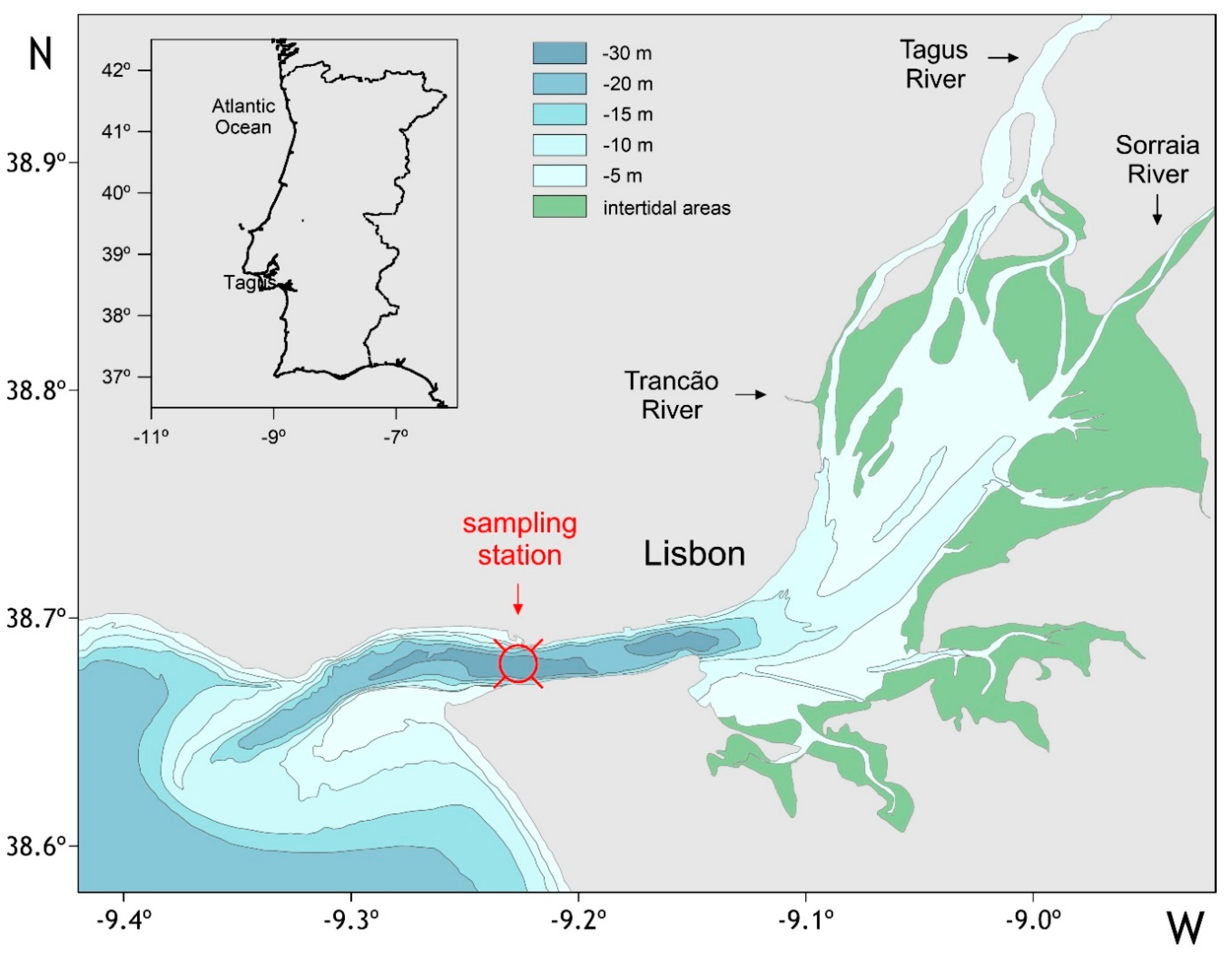
2.1. Study Area

The Tagus estuary is located on the densely populated west coast of Portugal, in the Iberian Peninsula (38°36′–39° N, 08°54′–09°24′ W) (Figure 1). The estuary is a relatively shallow and wide mesotidal lagoon-type estuary, connected with the Atlantic Ocean via a narrow and deep channel. It has extensive intertidal areas that comprise 20 to 40% of its total inner estuarine area. A fringe of salt marsh vegetation, covering approximately 13 km2, occupies the upper littoral zone. Hydrographic conditions are mainly determined by a considerable riverine input and the inflow of saline water from the Atlantic. Saline waters can be transported from 60 to 120 m depth since the coastal adjacent area is subjected to frequent upwelling events. The main freshwater source is the Tagus River with flows varying monthly from ~145 to ~815 m3∙s–1 [15], and other less important riverine discharges as the Sorraia and Trancão rivers. There are also a significant number of effluents from urban, industrial, and agricultural sources. The residence time of the waters in the estuary varies between 26 and 8 days [15]. Such features lead to a pronounced river plume extending in the coastal area [16]. Besides the fresh water inlets, an important driver of this mesotidal system hydrodynamics is the astronomic tide with a dominant semidiurnal period and maximum amplitude reaching 4.8 m in spring tide. Additionally, storm surges favoring a significant elevation of the water level (relative to astronomical tide) caused by meteorological forcing are reported to be frequent in the Tagus estuary lower section [17,18]. Wind predominance is from the south and southwest during winter, rotating progressively to the northwest and north during spring, and maintaining this direction throughout summer.

2.2. Sampling

Sampling was performed at a fixed station located in the lower section of the Tagus estuary (38°41.34′ N, 09°13.39′ W) (Figure 1). The lower estuary is connected to the coastal area by a channel, with depths over 30 m, having Lisbon (the Portuguese capital city) on its right bank. Sampling was conducted from February to December 2007 covering four seasons and included two tidal conditions (neap and spring). Surface water sampling (~1 m) was carried out at neap and spring tide every hour (approximately 13 h) with a Niskin horizontal bottle and a conductivity–temperature–depth (CTD) probe. A total of 101 observations were recorded. Sampling dates, hydrological information, and meteorological conditions are detailed in Table 1.

2.3. Meteorological Data

Wind speed and direction were measured in situ with a Vaisala® meteorological station (Datalogger Campbell Scientific CR510) (Campbell Scientific, Logan, UT, USA) coupled with a MetOne 034A (Campbell Scientific, Logan, UT, USA) anemometer. Continuous measurements were acquired with 1-min intervals at 11 m height. Wind speed was referenced to a height of 10 m (u10) [19] and a standard deviation of ±2 m∙s−1 was assumed as the wind speed error. Atmospheric CO2 data were measured at the Terceira Island’s reference station (Azores, Portugal, 38.77° N, 27.38° W), as part of the network of the National Oceanic and Atmospheric Administration (NOAA)/Climate Monitoring and Diagnostics Laboratory (CMDL)/Carbon Cycle Greenhouse Gases Group (CCGG) [20]. Dickson et al. [21] algorithms were used to convert observed atmospheric CO2 content in mole fraction (in dry air) to wet air values. Direct measurements of atmospheric CO2 partial pressure made on-board was only available for some sampling periods. Significant correlations were found out between Terceira data and shipboard data (r2 = 0.910, p < 0.05, n = 45) and the discrepancies occurred only between 3 and 13 µatm. The impact of using Terceira data on this study were considered negligible.

2.4. In Situ Measurements

Temperature (T) and salinity (S) parameters were determined in situ with a CTD Aanderaa (Bergen, Norway) probe. Salinity was calibrated with an AutoSal (OSIL, Hampshire, UK) salinometer using IAPSO standard seawater, with a variation coefficient of 0.003%. pH was measured immediately after sample collection at 25° C, using a Metrohm 704 (Metrohm, Herisau, Switzerland) pH-meter and a combination electrode (Metrohm) standardized against 2-amino-2-hydroxymethyl-1,3-propanediol seawater buffer (ionic strength of 0.7 M), at a precision of 0.005 pH units [21].

2.5. Chemical Analysis

Chlorophyll a (Chl a) was determined by filtering triplicate aliquots of ~150 mL water through Whatman GF/F(Sigma-Aldrich, Kawasaki, Japan) filters (0.7 µm) under a 0.2 atm vacuum, and immediately frozen and later extracted in 90% acetone for analysis in a fluorometer Hitachi F-7000 (Hong Kong, China), calibrated with commercial solutions of Chl a (Sigma-Aldrich, Kawasaki, Japan). The variation coefficient was 1.8%. Dissolved oxygen (DO) was analyzed following the Winkler method [22] using a whole-bottle manual titration, and the coefficient of variation associated with the method ranged from 0.08 to 0.25%. Total alkalinity (TA) samples were filtered through Whatman GF/F (0.7 μm) filters, fixed with HgCl2 and stored (refrigerated not frozen) until use. Samples were then titrated automatically with HCl (~0.25 M HCl in a solution of 0.45 M NaCl) past the endpoint of 4.5 [21], with an accuracy of ±2 μmol∙kg−1. The respective accuracy was controlled against certified reference material (batch 77, Marine Physical Laboratory, Scripps Institution of Oceanography, San Diego, CA, USA). Measured TA values (2260.91 µmol∙kg−1) differ from 2.7% from the theoretical values (2199.33 µmol∙kg−1).

2.6. Estimated Parameters

Current velocity and tidal height data at the Tagus estuary were calculated by running the MOHID model (information online at www.mohid.com) in hindcast mode, prescribing real forcing for river discharge, tide, and wind. The MOHID Water Modelling System is a 3D marine modelling platform that has been applied to the Tagus estuary in simultaneous hydrodynamic and biogeochemical studies (e.g., [16,23,24,25]). pH values corrected to in situ temperature were calculated from TA and in situ pH and temperature [26], using the carbon dioxide constants of Millero et al. [27]. TA values were normalized to a salinity of 35, being designated as nTA. Seawater pCO2 was calculated from in situ temperature, corrected pH and TA using the carbonic acid dissociation constants given by Millero et al. [27] and the CO2 solubility coefficient of Weiss, s [28]. Errors associated with pCO2 calculations were estimated to be ±10 µatm (accumulated errors on TA and pH).
The air–water CO2 fluxes (CO2 Flux) were computed according to the following equation [21]:
CO2 Flux = k·s·ΔpCO2 (mmol CO2 m−2∙d−1),
where k is the gas transfer velocity and ΔpCO2 is the air–water difference of pCO2. Positive CO2 flux indicates the emission of CO2 from water to the atmosphere and negative indicates otherwise. To determine the most likely value for k, calculations were based on a set of parameterizations: (1) Carini et al. [29] relationship (hereinafter referred to as C96), based on a SF6 release experiment in the Parker River estuary; (2) Raymond and Cole [30] relationship (hereinafter referred to as RC01), based on a compilation of published k600 values in various rivers and estuaries using different methodologies (floating chamber, natural tracers (CFC, 222Rn) and purposeful tracer SF6); and (3) Borges et al. [31] relationship (hereinafter referred to as B04) based on floating dome CO2 measurements in the Scheldt estuary, taking into account the contribution of the water current from the conceptual relationship of O’Connor and Dobbins [32].
All exploratory analysis and statistical modelling were implemented using the statistical software R 2.7.1 (Insightful Corp., 1999). A logarithmic transformation of the response variable pCO2 to linearity was necessary in order to perform subsequent analyses (Shapiro–Wilk test for normality, p < 0.05). The ANOVA (Analysis of Variance) was tested for significant differences in the following factors: tide (2 levels, neap and spring), tidal current (2 levels, ebb and flood), hours (variable was categorized into 3 levels, morning, noon, and afternoon), and season (4 levels, spring, summer, autumn, and winter). All explanatory variables were considered statistically different at a significance level of 0.05. Model building by variable selection was necessary to eliminate multicollinearity between independent variables. The backward elimination procedure was applied to obtain an ideal subset model. This method entered all four factors and their first-order effects (interactions between factors). Non-significant variables were removed according to the Akaike information criterion (AIC) [33].
A generalized linear model (GLM) with a log link function was applied to the entire data set to estimate the effects of various environmental variables (S, T, DO, and Chl a) on the response variable pCO2. The GLM, after a backward selection using the AIC, included the following factors: season, tide, tidal sequence, hours, and three interactions (between season and tide, season and tidal sequence, and hours and tide). When applying one-way ANOVAs for each of the four factors, the season and the tide were considered statistically significant (p < 0.05). An analysis of deviance was performed to assess the goodness-of-fit of the model.

3. Results

Ranges for measured physical-chemical and biological parameters are presented in Table 2.

3.1. Hydrodynamics

Generally, the Tagus river inputs reflect the common pattern of a mid-latitude system, with higher discharges in winter and lower ones in spring/summer (Table 1), despite the high degree of hydrological regime regularization imposed by a significant number of dams upstream. However, a relatively high discharge (109 m3∙s−1) at neap tide was noticed during summer. Inversely, reduced river discharges of only 17–18 m3∙s−1 were observed in autumn (Table 1). The impact of river inflows on the temperature and salinity at the estuary channel is depicted in the T-S diagram (Figure 2). Colder waters were observed in winter and autumn, whereas warmer waters were detected during the productive period (spring and summer). The occurrence of a relatively intense discharge in winter (370 m3∙s−1; Table 1) resulted in lower salinities (Table 2; Figure 2), whereas the exceptional high discharge in summer (Table 1) produced a decrease in salinity (Table 2; Figure 2). Tidal amplitude (Table 1) under neap conditions varied between 1.3 m (winter) and 2.1 m (summer) and under spring conditions between 3.0 m (summer) and 3.9 m (spring).

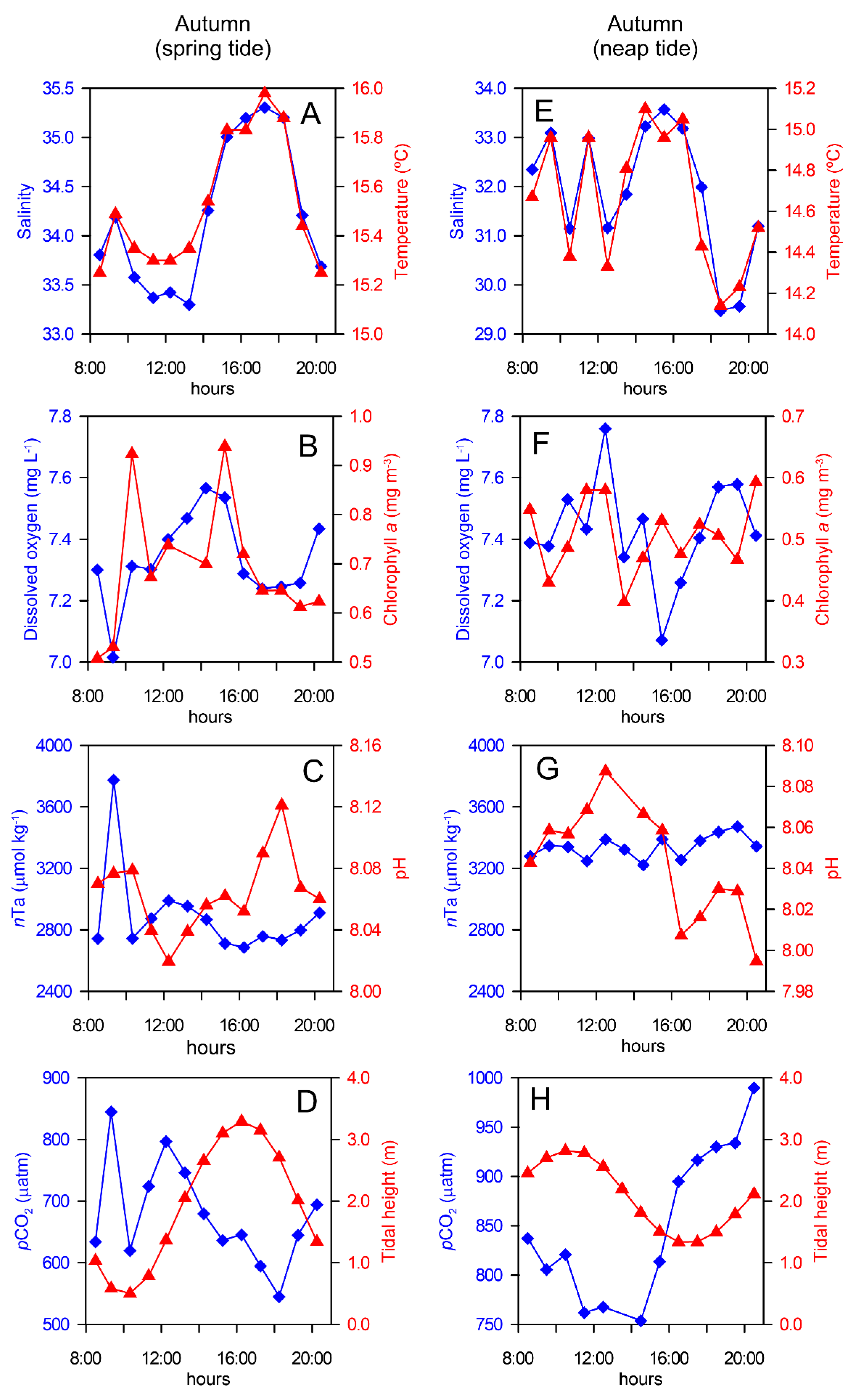
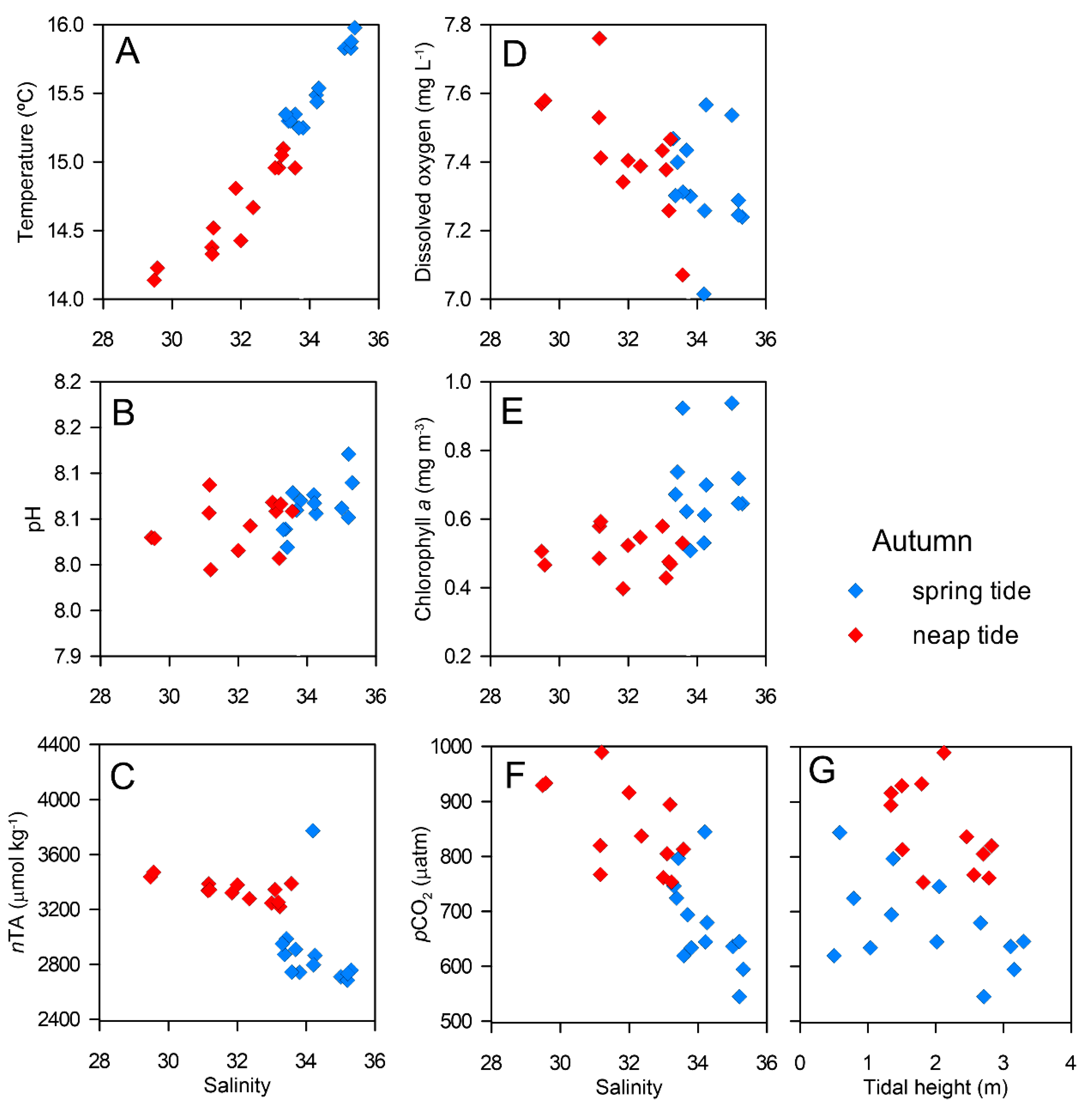
3.2. Tidal Variability

Data were recorded in the fixed station in autumn 2007, when river discharge reached the lowest flow values under both tide conditions (Table 1), to assess the semidiurnal tidal variability of pCO2 in the estuary. Figure 3 shows the semidiurnal tidal cycle effect on T, S, DO, Chl a, nTA, pH, and pCO2 parameters at spring and neap tide.
Most sampling campaigns were carried out at flood during the spring tide. Results showed that salinity tracked the tidal advection with its maximum and minimum practically coincident with high and low tide (Figure 3A). The semidiurnal tidal cycle was followed by other variables as well. In general, maximum values of T, Chl a, and pH were attained simultaneously with minimum values of nTA at high tide (Figure 3A–C). This occurrence indicated that warmer, and biologically more productive marine waters impoverished in alkalinity, were transported to the estuary by the flooding tidal current. During neap tide most of the sampling occurred at ebb, but a slight lag between the salinity maximum and the high tide was observed. Minima values of S and T were reached at the initial hours of flood (Figure 3E). Such features were reflected on the trends of Chl a, DO, pH, and nTA (Figure 3F,G). The plots of temperature, pH, nTA, DO, and Chl a versus salinity (Figure 4) in autumn revealed that warmer and more productive offshore waters with higher pH dominated the lower estuary at flood (spring tide). The influence of colder, more oxygenated, less productive, and carbonate-enriched Tagus estuarine waters was observed during ebb (Figure 4A–E).
Estuarine levels of CO2 follow the tidal cycle in autumn: an increase in pCO2 values at ebb, both under spring and neap tide conditions (Figure 3D,H), indicates the transport of CO2-enriched estuarine waters to the coast.
Such features are also evidenced on the plots of pCO2 against salinity (Figure 4F) and, although not so obviously, with tidal elevation (Figure 4G). For this period of the year, the tidal influence on the variability of pCO2 was statistically significant (Fisher’s test, p < 0.001, n = 26). Considering all samples for 2007 (n = 101), the difference of the average ranges of tidal pCO2 was 208 µatm. This value was calculated as the average of the difference between the lower and higher values at each tidal cycle.

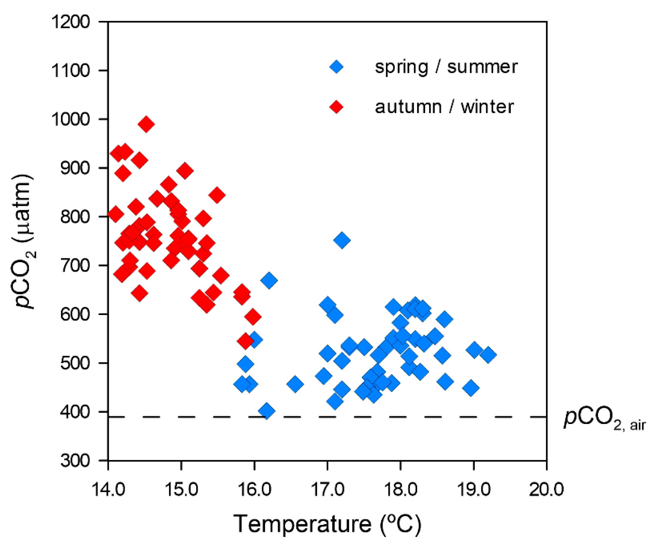
3.3. Seasonal Variability

Seasonal variation is detected in all the analyzed parameters, a pattern detected in the box plots with the physical-chemical and biological water properties for the four periods sampled in 2007 (Figure 5). Temperature and salinity increased from winter to spring/summer. Temperature ranged from 14.1 to 19.2 °C and salinity from 21.2 to 35.3 (Figure 5A,B; Table 2). Salinity values were strongly controlled by river discharges and showed considerable variability (Figure 5B; Table 1), showing lower values in winter. Maximum Chl a concentrations were measured during the productive period, peaking at 10.2 mg∙m−3, reached in spring tide, associated with high variability. During the non-productive period, the values of Chl a hardly attained 1 mg∙m−3 (Figure 5C; Table 2). pH varied from 7.88 to 8.19, with the highest values recorded during spring and summer (Figure 5D; Table 2). The lowest values of nTA were also attained during spring and summer (Figure 5E, Table 2).
Mean values of pCO2 ranged from 402 to 990 µatm throughout the year and displayed maximum values during the non-productive period (Figure 5F; Table 2). The amplitude of pCO2 seasonal signal was 588 µatm. The relationship between surface water pCO2 and temperature (Figure 6) showed different patterns regarding the productive and non-productive periods: pCO2 was higher at the low temperature during autumn and winter, and showed the opposite pattern during the productive period, with lower pCO2 associated with higher temperatures.
The effect of different environmental variables (S, T, DO, and Chl a) on pCO2 response was assessed by applying the GLM to the complete data set, and the following equation was obtained:
log (E(pCO2) = 7.50 + 0.05 × DO − 0.08 × T – 0.04 × Chl a,
where E is the expected (mean) value of pCO2 in µatm, T in °C, DO in mg∙L−1, and Chl a in mg∙m−3. The respective model explains 69.3% of pCO2 variability, where temperature and chlorophyll a accounted for 58.4% and 7.6% deviance, respectively (Table 3).

3.4. Air–Water CO2 Fluxes

Daily average CO2 air–water fluxes for each tidal cycle sampling, and respective fluxes against the wind speed, are presented in Figure 7. These values were estimated according to the three mentioned parameterizations (Section 2.6). In general, the highest fluxes were observed during more intense wind speed, except for three samplings during the productive period (Figure 7B). The averaged CO2 fluxes estimated by the three parameterizations ranged from 2 mmol∙m−2∙d−1 in spring to 56 mmol∙m−2∙d−1 in winter, following a seasonal pattern (Fisher’s test, p < 0.001, n = 101). In general, the lowest fluxes were obtained when applying the C96 relationship, followed by RC01 and B04 with the highest estimates (Figure 7A).
On average, the fluxes estimated by the RC01 and B04 algorithms differed from those obtained from C96, respectively by 22% and 36%. An exception was observed when the wind speed was low, as in spring (24 April) (Figure 7A).

4. Discussion

4.1. Tidal Variability

The evolution of monitored environmental variables was distinct along tidal cycles and under different tide conditions (neap/spring) in the Tagus estuary, clearly revealing significant tidal variability. These patterns were shaped by the effects of tide amplitude alone, or in combination with a tidal asymmetric behavior, since flood is typically one hour longer than ebb in the estuary, leading to higher current velocities during ebbs [34]. An examination of the temporal distribution of environmental variables together with tidal data from autumn 2007 revealed some typical features of dynamics of the estuary, namely, a dominant east-west current transporting CO2-rich water from the inner to the lower estuary, while the reverse tidal current imported saltier and more productive (phytoplankton-rich) seawater into the estuary (Figure 3 and Figure 4). When river discharge was minimum (autumn 2007), salinity amplitude in surface water varied between 1.6 and 8.4 along a 13-h cycle. Considering that vertical stratification was absent (corroborated by CTD profiles, data not shown), variations in salinity were mostly controlled by horizontal mixing and advection. The effect of such physical processes along the tidal cycle was noticed in the concentration trends of the water properties. Similar water advection control was also reported in the Guadalquivir estuary (SW Spain), for properties such as TA, dissolved inorganic carbon and apparent oxygen utilization [35].
As previously noted, the range of pCO2 variation also suggested that this property changed as a function of tide amplitude. Higher variability was, in general, observed in association with spring tide data (Figure 5F). For example, when higher tide amplitude occurred (Δ = 2.5 m) on 17 April (Table 1, spring data), the amplitude of pCO2 over the tidal cycle was 330 µatm. By contrast, on 24 April when the tidal range was only 1.4 m (Table 1), pCO2 amplitude was only 100 µatm. Differences in variability were not, however, so significant in summer and autumn, a pCO2 amplitude difference of ~21% being observed between tides, contrasting with 70% obtained in spring.
The tendency of elevated pCO2 at low tides in the Tagus channel can also be attributed to biogeochemical processes, namely, the inorganic carbon respiration in the upper/central estuary. High loadings of organic matter and nutrients (data not shown) originating in the shallow inner estuarine areas could reach the study site at low tide, supporting in situ production of CO2. Several authors have concluded that benthic mineralization processes can be a major source of CO2 to the water column in different coastal systems (e.g., Hammond et al. [36], Cai et al. [37], and Forja et al. [38]). The Tagus estuary is no exception [39,40,41,42]. Moreover, the relatively low correlation between pCO2 and Chl a (r = −0.574, p < 0.05) agrees with the GLM results (6.5% deviance for Chl a).
The thermodynamic impact of temperature on pCO2 variation using an average temperature for each sampling period [43] yields a correction of 2% of the measured value on average, suggesting that the difference in the magnitude of pCO2 between tides is not affected by thermodynamic effects. Hence, the variability of CO2 on a tidal scale in the Tagus estuary is essentially influenced by variables (e.g., salinity) and processes such as tidal advection and horizontal mixing of the two water masses—estuarine water and oceanic water. Biological activity seems to account to a lesser extent to such variability. More accurate studies on the dynamics of the lower Tagus estuary would be necessary to expand on these assumptions. However, such studies require an increase in the sampling frequency and/or the presence of mooring buoys with physicochemical sensors, both limiting by their operational and financial costs.

4.2. Seasonal Variability

All studied variables reflect typical seasonal variations of a mid-latitude system (Figure 5). The highest observed pCO2 value in winter was 890 µatm, corresponding to an oversaturation of ~230% of pCO2 (calculated using the annual mean of atmospheric pCO2, air of 389.2 µatm). During spring and summer pCO2 values dropped to 402 µatm and increased again to a maximum of 990 µatm in autumn, showing an oversaturation of ~250%. These values fall within the ranges reported for other coastal systems [9,11,44].
The GLM applied to the entire data set (n = 101; Table 3) points to the thermodynamic effect of temperature and, to a lesser extent, to the biological activity, as the main factors controlling pCO2 variability. The slope of the plot for pCO2 vs. T is 19.4 µatm∙°C−1 (r = 0.487, p < 0.05) in summer (Figure 6), close to the thermodynamic value of 13 µatm∙°C−1 determined empirically by Takahashi et al. [43]. This suggests that pCO2 is independent of temperature in that period of the year. The negligible phytoplankton production might have contributed to the elevated pCO2 values during autumn and winter. Actually, when a statistical GLM was exclusively applied to the productive period data set (n = 52), pCO2 variability was found to be satisfactorily explained by chlorophyll a and dissolved oxygen (33% of the variability), therefore associated with biological activity. Although the interpretation of GLM results should be done with caution due to the relatively low number of observations under analysis, the decrease of pCO2 values during the productive period is, most likely, the result of phytoplankton blooms and the related photosynthetic assimilation of CO2.
Studies on the inorganic carbon systems in coastal areas have reported high pCO2 associated with upwelled waters, suggesting that upwelling is a source of both nutrient-rich and high CO2 levels [45,46]. This occurrence, however, is not evident in the results, probably due to the strong influence of inner estuarine waters, frequently characterized by the same combination of nutrients and high pCO2.

4.3. Air–Water CO2 Exchange

The results showed significant variation in the magnitude of estimated CO2 fluxes emitted from the Tagus, depending on the algorithm used to estimate the gas transfer velocity (Figure 7). Lower CO2 fluxes are obtained using the C96 algorithm, due to the lower k values, probably because of strong fetch limitation and low tidal currents in the Parker River estuary [29]. Fluxes estimated by the three algorithms differed significantly, similarly to what has been observed in numerous CO2 studies [31,47,48]. It has been pointed out that the greatest source of uncertainty in the calculation of gas fluxes arises from the rate term k in both open and coastal environment processes [31]. In shallow coastal sites, however, where important sources of turbulence exist (e.g., boundary friction, current velocity), one or more of these processes may control the air–water exchanges. In macrotidal estuaries specifically, tidal currents were found to significantly affect k, especially under low wind conditions [31,48,49,50].
Inherent differences in various measurement techniques is another source of uncertainty, leading to the emergence of new alternatives for standard formulations for the solubility and gas transfer velocities across air–water surfaces (e.g., [51,52,53,54]). However, such formulations require more comprehensive simulations of atmosphere–ocean interactions, and further calibration and validation. For this reason, some authors [31,48,49,50,55] concluded that a simple parameterization of k as a function of wind speed should be site-specific in estuaries, and that the use of generic relationships to estimate air–water fluxes could lead to substantial errors. Nevertheless, the variability of the calculated air–water CO2 fluxes throughout the tidal cycle is larger (50–80%) than the variability of fluxes using different parameterizations, as a result of fluctuations in both ΔpCO2 and wind speed. Hence, for estimates of CO2 sinks and sources in the Tagus estuary, or for areas and seasons characterized by strong diurnal cycles of temperature and productivity, it is preferable to perform measurements that account for short time variability.
Despite the different values coming from the various parameterizations, CO2 fluxes show a clear seasonal pattern. The highest fluxes were attained in winter (24.5–65.5 mmol∙m−2∙d−1) and the lowest in spring (0.4–21.3 mmol∙m−2∙d−1). Another common feature was the highest emissions, coincident with the highest wind speed (Figure 7B), indicating that CO2 exchanges were, to a large extent, driven by wind. Some exceptions were noticed during the productive period (Figure 7B), when high wind speed was associated with a decrease in pCO2. This phenomenon is explained by low ΔpCO2 (Figure 5F), most likely due to carbon uptake by primary producers, as suggested by the higher values of chlorophyll a observed for that period (spring and summer, Figure 5C).
Throughout the year 2007, the part of the Tagus estuary directly influenced by marine waters acted as a weak source of CO2 to the atmosphere, at an average rate of 7.2 mol∙C∙m−2∙year−1 (average value for the three parameterizations). This value is within the range reported for near-shore ecosystems [9,11].

5. Conclusions

Several interrelated factors and processes, occurring at tidal and seasonal scales, control the CO2 dynamics in the lower estuarine areas under direct influence of marine waters. The generalized linear model applied to the lower Tagus estuary 2007 data set (n = 101) explained 69.3% of the pCO2 variability, pointing to the thermodynamic effect of temperature and biological activity as the most important processes in CO2 dynamics. The tidal variation of pCO2 was found to correspond to ~35% of the seasonal range of variability, emphasizing the importance of tidal fluctuations on carbon variability in the estuary. As a consequence, the use of seasonal data sets without daily quantifications and characterizations of tidal trends may lead to significant errors in annual carbon fluxes and budget calculations. Lower pCO2 values consistently occurred in high tides. Thus, the use of “single-point” monthly or seasonal data collected during low tide to calculate a CO2 gas-flux budget might overestimate the flux of CO2 to the atmosphere at this specific location. Similarly, the use of monthly or seasonal data collected during high tides at high solar radiation could underestimate the flux of CO2 to the atmosphere.
Overall, at the time of sampling, the lower Tagus estuary acted as a relatively weak source of CO2 to the atmosphere, at an average rate of 7.2 mol∙m−2∙year−1 (average value for the three parameterizations), with highest fluxes in winter. On average, the fluxes estimated by the RC01 and B04 algorithms differed from those obtained from C96, respectively by 22% and 36%. Despite the different values coming from the various parameterizations, CO2 fluxes showed a clear seasonal pattern: highest fluxes in winter (24.5–65.5 mmol∙m−2∙d−1) and lowest in spring (0.4–21.3 mmol∙m−2∙d−1). Another common feature was the highest emissions to be, in general, coincident with the highest wind speed, indicating that CO2 exchanges are, to a large extent, driven by wind speed.
The results strongly illustrate the need for higher temporal resolution data for the assessment of coastal carbon fluxes for this estuary, supporting previous similar claims by other researchers referring to other ecosystems [14,46,56,57,58]. Therefore, the combination of seasonal point and transect evaluations with periodic diurnal measurements of system parameters will improve annual carbon budget calculations and may provide better numeric modelling of water quality. Furthermore, it may provide additional insights on why the continental shelves might have switched from a source to a sink of CO2 over the last century [59].
Finally, the methodological approach presented here can be improved in future works, to reflect recent findings in the study of CO2 air–water fluxes. Such enhancements can include, for example, the calculation of the upwelling index to obtain a better insight on the influence of this source of CO2 at the monitored areas, as done by Ribas-Ribas et al. [45], as well as the estimate of the uncertainty propagation associated with pCO2 calculations, as proposed by Orr et al. [60].

Author Contributions

Conceptualization, A.P.O. and G.C.; Data curation, A.P.O.; Formal analysis, A.P.O., T.P.-F., and M.M.; Funding acquisition, A.P.O., G.C., and M.M.; Investigation, A.P.O. and M.M.; Methodology, A.P.O., G.C., and T.P.-F.; Project administration, G.C.; Writing—original draft preparation, A.P.O. and M.M.; Writing—review and editing, A.P.O., G.C., and M.M.

Funding

Ana Paula Oliveira was financed by a PhD grant from FCT—Foundation for Science and Technology under contract SFRH/BD/28507/06, and by E.U. Project POPesca/MARE 22-05-01-FDR 00015. Marcos Mateus was funded by ERDF Funds of the Competitiveness Factors Operational Programme—COMPETE and by national funds from the FCT—Foundation for Science and Technology project UID/EEA/50009/2013.

Acknowledgments

The authors would like to thank Ana Cristina Oliveira, Célia Gonçalves, Conceição Araújo, Isaura Franco, João Garcês, Luís Palma Oliveira, Maria Rosa Pinto, Sara Costa, and Vanda Franco for sampling, technical, and analytical assistance.

Conflicts of Interest

The authors declare no conflict of interest.

References

  1. Kemp, W.M.; Smith, E.M.; Marvin-DiPasquale, M.; Boynton, W.R. Organic carbon balance and net ecosystem metabolism in Chesapeake Bay. Mar. Ecol. Prog. Ser. 1997, 150, 229–248. [Google Scholar] [CrossRef] [Green Version]
  2. Gattuso, J.P.; Frankignoulle, M.; Wollast, R. Carbon and carbonate metabolism in coastal aquatic ecosystems. Annu. Rev. Ecol. Syst. 1998, 29, 405–434. [Google Scholar] [CrossRef]
  3. Gazeau, F.; Smith, S.V.; Gentili, B.; Frankignoulle, M.; Gattuso, J.P. The European coastal zone: Characterization and first assessment of ecosystem metabolism. Estuar. Coast. Shelf Sci. 2004, 60, 673–694. [Google Scholar] [CrossRef]
  4. Hopkinson, C.S.J.; Smith, E.M. Estuarine respiration: An overview of benthic, pelagic and whole system respiration. In Respiration in Aquatic Ecosystems; del Giorgio, P.A., Williams, P.J.L., Eds.; Oxford University Press: Oxford, UK, 2005; pp. 123–147. [Google Scholar]
  5. Cai, W.-J. Estuarine and Coastal Ocean Carbon Paradox: CO2 Sinks or Sites of Terrestrial Carbon Incineration? Annu. Rev. Mar. Sci. 2011, 3, 123–145. [Google Scholar] [CrossRef]
  6. Laruelle, G.G.; Dürr, H.H.; Slomp, C.P.; Borges, A.V. Evaluation of sinks and sources of CO2 in the global coastal ocean using a spatially-explicit typology of estuaries and continental shelves. Geophys. Res. Lett. 2010, 37, 15. [Google Scholar] [CrossRef]
  7. Laruelle, G.G.; Dürr, H.H.; Lauerwald, R.; Hartmann, J.; Slomp, C.P.; Goossens, N.; Regnier, P.A.G. Global multi-scale segmentation of continental and coastal waters from the watersheds to the continental margins. Hydrol. Earth Syst. Sci. 2013, 17, 2029–2051. [Google Scholar] [CrossRef]
  8. Chen, C.T.A.; Huang, T.H.; Chen, Y.C.; Bai, Y.; He, X.; Kang, Y. Air-sea exchanges of CO2 in the world’s coastal seas. Biogeosciences 2013, 10, 6509–6544. [Google Scholar] [CrossRef]
  9. Chen, C.-T.A.; Borges, A.V. Reconciling opposing views on carbon cycling in the coastal ocean: Continental shelves as sinks and nearshore ecosystems as sources of atmospheric CO2. Deep Sea Res. Part II Top. Stud. Oceanogr. 2009, 56, 578–590. [Google Scholar] [CrossRef]
  10. Chen, D.; Zuo, T.; Chen, J.N. Variation of Air-Sea Heat Fluxes over the Kuroshio Area and Its Relationship with the Flood Season Precipitation in Qingdao. In Proceedings of the 2013 IEEE International Geoscience and Remote Sensing Symposium, Melbourne, Australia, 21–26 July 2013. [Google Scholar]
  11. Oliveira, A.P.; Cabeçadas, G.; Pilar-Fonseca, T. Iberia coastal ocean in the CO2 sink/source context: Portugal case study. J. Coast. Res. 2012, 28, 184–195. [Google Scholar] [CrossRef]
  12. Frankignoulle, M.; Abril, G.; Borges, A.; Bourge, I.; Canon, C.; DeLille, B.; Libert, E.; Theate, J.M. Carbon dioxide emission from European estuaries. Science 1998, 282, 434–436. [Google Scholar] [CrossRef]
  13. Abril, G.; Etcheber, H.; Borges, A.V.; Frankignoulle, M. Excess atmospheric carbon dioxide transported by rivers into the Scheldt estuary. Comptes Rendus de l’Académie des Sci. Ser. IIA Earth Planet. Sci. 2000, 330, 761–768. [Google Scholar] [CrossRef] [Green Version]
  14. Dinauer, A.; Mucci, A. Spatial variability in surface-water pCO2 and gas exchange in the world’s largest semi-enclosed estuarine system: St. Lawrence Estuary (Canada). Biogeosciences 2017, 14, 3221–3237. [Google Scholar] [CrossRef]
  15. Braunschweig, F.; Martins, F.; Chambel, P.; Neves, R. A methodology to estimate renewal time scales in estuaries: The Tagus Estuary case. Ocean Dyn. 2003, 53, 137–145. [Google Scholar] [CrossRef]
  16. Oliveira, A.; Mateus, M.; Cabecadas, G.; Neves, R. Water-air CO2 fluxes in the Tagus estuary plume (Portugal) during two distinct winter episodes. Carbon Balance Manag. 2015, 10, 2. [Google Scholar] [CrossRef]
  17. Gama, C.; Dias, J.; Ferreira, O.; Taborda, R. Analysis of storm surge in Portugal, between June 1986 and May 1988. In Proceedings of the Littoral 94, Lisboa, Portugal, 26–29 September 1994; pp. 381–387. [Google Scholar]
  18. Sebastião, P.; Guedes Soares, C.; Alvarez, E. 44 years hindcast of sea level in the Atlantic Coast of Europe. Coast. Eng. 2008, 55, 843–848. [Google Scholar] [CrossRef]
  19. Johnson, H.K. Simple expressions for correcting wind speed data for elevation. Coast. Eng. 1999, 36, 263–269. [Google Scholar] [CrossRef]
  20. Conway, T.J.; Lang, P.M.; Masarie, K.A. Atmospheric Carbon Dioxide Dry Air Mole Fractions from the NOAA ESRL Carbon Cycle Cooperative Global Air Sampling Network, 1968–2006. Available online: ftp://ftp.cmdl.noaa.gov/ccg/co2/flask/event/ (accessed on 15 April 2008).
  21. Dickson, A.G.; Sabine, C.L.; Christian, J.R. Guide to Best Practices for Ocean CO2 Measurements; North Pacific Marine Science Organization: Sidney, BC, Canada, 2007; p. 191. [Google Scholar]
  22. Carrit, D.E.; Carpenter, J.H. Comparison and evaluation of currently employed modifications of the Winkler method for determining oxygen in seawater. A NASCO Report. J. Mar. Res. 1966, 24, 286–318. [Google Scholar]
  23. Martins, F.; Leitão, P.; Silva, A.; Neves, R. 3D modelling in the Sado estuary using a new generic vertical discretization approach. Oceanol. Acta 2001, 24, 51–62. [Google Scholar] [CrossRef]
  24. Vaz, N.; Mateus, M.; Dias, J.M. Semidiurnal and spring-neap variations in the Tagus Estuary: Application of a process-oriented hydro-biogeochemical model. J. Coast. Res. 2011, 64, 1619–1623. [Google Scholar]
  25. Mateus, M.; Vaz, N.; Neves, R. A process-oriented model of pelagic biogeochemistry for marine systems. Part II: Application to a mesotidal estuary. J. Mar. Syst. 2012, 94, 90–101. [Google Scholar] [CrossRef]
  26. Hunter, K.A. The temperature dependence of pH in surface seawater. Deep Sea Res. Part I Oceanogr. Res. Pap. 1998, 45, 1919–1930. [Google Scholar] [CrossRef]
  27. Millero, F.J.; Graham, T.B.; Huang, F.; Bustos-Serrano, H.; Pierrot, D. Dissociation constants of carbonic acid in seawater as a function of salinity and temperature. Mar. Chem. 2006, 100, 80–94. [Google Scholar] [CrossRef]
  28. Weiss, R.F. Carbon dioxide in water and seawater: The solubility of a non-ideal gas. Mar. Chem. 1974, 2, 203–215. [Google Scholar] [CrossRef]
  29. Carini, S.; Weston, N.; Hopkinson, C.; Tucker, J.; Giblin, A.; Vallino, J. Gas exchange rates in the Parker River estuary, Massachusetts. Biol. Bull. 1996, 191, 333–334. [Google Scholar] [CrossRef]
  30. Raymond, P.A.; Cole, J.J. Gas exchange in rivers and estuaries: Choosing a gas transfer velocity. Estuaries 2001, 24, 312–317. [Google Scholar] [CrossRef]
  31. Borges, A.V.; Delille, B.; Schiettecatte, L.S.; Gazeau, F.; Abril, G.; Frankignoulle, M. Gas transfer velocities of CO2 in three European estuaries (Randers Fjord, Scheldt, and Thames). Limnol. Oceanogr. 2004, 49, 1630–1641. [Google Scholar] [CrossRef]
  32. O’Connor, D.J.; Dobbins, W.E. Mechanism of reaeration in natural streams. Trans. Am. Soc. Civ. Eng. 1958, 123, 641–684. [Google Scholar]
  33. Hastie, T.J.; Pregibon, D. Generalized linear models. In Statistical Models in S; Chambers, J.M., Hastie, T.J., Eds.; Chapman & Hall/CRC: Boca Raton, FL, USA, 1993. [Google Scholar]
  34. Fortunato, A.; Oliveira, A.; Baptista, A.M. On the effect of tidal flats on the hydrodynamics of the Tagus estuary. Oceanol. Acta 1999, 22, 31–44. [Google Scholar] [CrossRef]
  35. De la Paz, M.; Gómez-Parra, A.; Forja, J. Inorganic carbon dynamic and air–water CO2 exchange in the Guadalquivir Estuary (SW Iberian Peninsula). J. Mar. Syst. 2007, 68, 265–277. [Google Scholar] [CrossRef]
  36. Hammond, D.E.; Giordani, P.; Berelson, W.M.; Poletti, R. Diagenesis of carbon and nutrients and benthic exchange in sediments of the Northern Adriatic Sea. Mar. Chem. 1999, 66, 53–79. [Google Scholar] [CrossRef]
  37. Cai, W.J.; Zhao, P.S.; Wang, Y.C. pH and pCO(2) microelectrode measurements and the diffusive behavior of carbon dioxide species in coastal marine sediments. Mar. Chem. 2000, 70, 133–148. [Google Scholar] [CrossRef]
  38. Forja, J.M.; Ortega, T.; DelValls, T.A.; Gómez-Parra, A. Benthic fluxes of inorganic carbon in shallow coastal ecosystems of the Iberian Peninsula. Mar. Chem. 2004, 85, 141–156. [Google Scholar] [CrossRef]
  39. Canário, J.P.; Vale, C.D.; Caetano, M.D.N. Distribution of monomethylmercury and mercury in surface sediments of the Tagus Estuary (Portugal). Mar. Pollut. Bull. 2005, 50, 1142–1145. [Google Scholar] [CrossRef]
  40. Brotas, V.; Catarino, F. Microphytobenthos primary production of Tagus estuary intertidal flats (Portugal). Netherland J. Aquat. Ecol. 1995, 29, 333–339. [Google Scholar] [CrossRef]
  41. Tobias, C.; Giblin, A.; McClelland, J.; Tucker, J.; Peterson, B. Sediment DIN fluxes and preferential recycling of benthic microalgal nitrogen in a shallow macrotidal estuary. Mar. Ecol. Prog. Ser. 2003, 257, 25–36. [Google Scholar] [CrossRef]
  42. Cabrita, M.T.; Brotas, V. Seasonal variation in denitrification and dissolved nitrogen fluxes in intertidal sediments of the Tagus estuary, Portugal. Mar. Ecol. Prog. Ser. 2000, 202, 51–65. [Google Scholar] [CrossRef] [Green Version]
  43. Takahashi, T.; Olafsson, J.; Goddard, J.G.; Chipman, D.W.; Sutherland, S.C. Seasonal variation of CO2 and nutrients in the high-latitude surface oceans—A comparative study. Glob. Biogeochem. Cycles 1993, 7, 843–878. [Google Scholar] [CrossRef]
  44. Borges, A.V.; Schiettecatte, L.S.; Abril, G.; Delille, B.; Gazeau, E. Carbon dioxide in European coastal waters. Estuar. Coast. Shelf Sci. 2006, 70, 375–387. [Google Scholar] [CrossRef] [Green Version]
  45. Ribas-Ribas, M.; Hernández-Ayón, J.M.; Camacho-Ibar, V.F.; Cabello-Pasini, A.; Mejia-Trejo, A.; Durazo, R.; Galindo-Bect, S.; Souza, A.J.; Forja, J.M.; Siqueiros-Valencia, A. Effects of upwelling, tides and biological processes on the inorganic carbon system of a coastal lagoon in Baja California. Estuar. Coast. Shelf Sci. 2011, 95, 367–376. [Google Scholar] [CrossRef]
  46. Ribas-Ribas, M.; Anfuso, E.; Gómez-Parra, A.; Forja, J.M. Tidal and seasonal carbon and nutrient dynamics of the Guadalquivir estuary and the Bay of Cádiz (SW Iberian Peninsula). Biogeosciences 2013, 10, 4481–4491. [Google Scholar] [CrossRef] [Green Version]
  47. Abril, G.; Borges, A.V. Carbon dioxide and methane emissions from estuaries. In Greenhouse Gases Emissions from Natural Environments and Hydroelectric Reservoirs: Fluxes and Processes; Tremblay, A., Varfalvy, L., Roehm, M., Garneau, M., Eds.; Springer-Verlag: New York, NY, USA, 2004; pp. 187–207. [Google Scholar]
  48. Borges, A.; Vanderborght, J.-P.; Schiettecatte, L.-S.; Gazeau, F.; Ferrón-Smith, S.; Delille, B.; Frankignoulle, M. Variability of the gas transfer velocity of CO2 in a macrotidal estuary (the Scheldt). Estuaries 2004, 27, 593–603. [Google Scholar] [CrossRef]
  49. Zappa, C.J.; McGillis, W.R.; Raymond, P.A.; Edson, J.B.; Hintsa, E.J.; Zemmelink, H.J.; Dacey, J.W.H.; Ho, D.T. Environmental turbulent mixing controls on air-water gas exchange in marine and aquatic systems. Geophys. Res. Lett. 2007, 34, 10. [Google Scholar] [CrossRef]
  50. Zappa, C.J.; Raymond, P.A.; Terray, E.A.; McGillis, W.R. Variation in surface turbulence and the gas transfer velocity over a tidal cycle in a macro-tidal estuary. Estuaries 2003, 26, 1401–1415. [Google Scholar] [CrossRef]
  51. Vieira, V.; Jurus, P.; Clementi, E.; Mateus, M. The FuGas 2.3 Framework for Atmosphere–Ocean Coupling: Comparing Algorithms for the Estimation of Solubilities and Gas Fluxes. Atmosphere 2018, 9, 310. [Google Scholar] [CrossRef]
  52. Bigdeli, A.; Hara, T.; Loose, B.; Nguyen, A.T. Wave Attenuation and Gas Exchange Velocity in Marginal Sea Ice Zone. J. Geophys. Res. Oceans 2018, 123, 2293–2304. [Google Scholar] [CrossRef]
  53. Shuiqing, L.; Dongliang, Z. Gas transfer velocity in the presence of wave breaking. Tellus B Chem. Phys. Meteorol. 2016, 68, 27034. [Google Scholar] [CrossRef] [Green Version]
  54. Wang, B.; Liao, Q.; Fillingham, J.H.; Bootsma, H.A. On the coefficients of small eddy and surface divergence models for the air-water gas transfer velocity. J. Geophys. Res. Oceans 2015, 120, 2129–2146. [Google Scholar] [CrossRef] [Green Version]
  55. Kremer, J.N.; Reischauer, A.; D’Avanzo, C. Estuary-specific variation in the air-water gas exchange coefficient for oxygen. Estuaries 2003, 26, 829–836. [Google Scholar] [CrossRef]
  56. Cai, W.J.; Pomeroy, L.R.; Moran, M.A.; Wang, Y.C. Oxygen and carbon dioxide mass balance for the estuarine-intertidal marsh complex of five rivers in the southeastern US. Limnol. Oceanogr. 1999, 44, 639–649. [Google Scholar] [CrossRef]
  57. Borges, A.V.; Frankignoulle, M. Daily and seasonal variations of the partial pressure of CO2 in surface seawater along Belgian and southern Dutch coastal areas. J. Mar. Syst. 1999, 19, 251–266. [Google Scholar] [CrossRef]
  58. Yates, K.K.; Dufore, C.; Smiley, N.; Jackson, C.; Halley, R.B. Diurnal variation of oxygen and carbonate system parameters in Tampa Bay and Florida Bay. Mar. Chem. 2007, 104, 110–124. [Google Scholar] [CrossRef]
  59. Laruelle, G.G.; Cai, W.-J.; Hu, X.; Gruber, N.; Mackenzie, F.T.; Regnier, P. Continental shelves as a variable but increasing global sink for atmospheric carbon dioxide. Nat. Commun. 2018, 9, 454. [Google Scholar] [CrossRef]
  60. Orr, J.C.; Epitalon, J.-M.; Dickson, A.G.; Gattuso, J.-P. Routine uncertainty propagation for the marine carbon dioxide system. Mar. Chem. 2018, 207, 84–107. [Google Scholar] [CrossRef]
Figure 1. Map of Tagus estuary (SW Portugal) showing the location of the fixed sampling station.
Geosciences 08 00460 g001
Figure 2. Temperature–salinity diagram for the surface waters sampled at the fixed station in 2007.
Geosciences 08 00460 g002
Figure 3. Tidal variation of: (A,E) salinity and temperature, (B,F) chlorophyll a and dissolved oxygen, (C,G) normalized alkalinity (nTA) and pH, and (D,H) CO2 partial pressure (pCO2) and tidal height, in spring and neap tide in the Tagus fixed station, for autumn 2007.
Geosciences 08 00460 g003
Figure 4. Autumn 2007 data for (A) temperature, (B) pH, (C) normalized alkalinity (nTA), (D) dissolved oxygen, (E) chlorophyll a, (F) CO2 partial pressure (pCO2), and (G) pCO2 versus tidal height.
Geosciences 08 00460 g004
Figure 5. Box plots of (A) temperature, (B) salinity, (C) chlorophyll a, (D) pH, (E) normalized alkalinity (nTA), and (F) CO2 partial pressure (pCO2) for the sampling periods at the Tagus fixed station. Values are median with quartiles in boxes, 90% confidence limits are shown as bars, and observations outside 90% confidence limits are shown as diamonds (outliers).
Geosciences 08 00460 g005
Figure 6. Distribution of CO2 partial pressure (pCO2) as a function of surface temperature for all sampling periods in the Tagus fixed station. The dashed horizontal line represents the mean atmospheric CO2 pressure (pCO2, air = 389.2 µatm) for the year 2007.
Geosciences 08 00460 g006
Figure 7. Average CO2 fluxes for (A) all seasons sampled during 2007, and (B) as a function of wind speed (u10). Positive values denote a flux from the water to the atmosphere. The values were calculated with three parameterizations: Carini et al. (1996) algorithm (C96), Raymond and Cole (2001) algorithm (RC01), and Borges et al. (2004a) algorithm (B04). Diamonds on panel A show average air–water fluxes for each parameterization.
Geosciences 08 00460 g007
Table 1. Sampling dates and ranges of hydrologic and wind data recorded for each sampling period in the Tagus estuary fixed station during 2007. Q represents Tagus river flow and u10 the wind speed referenced to a height of 10 m (expressed in m∙s−1, see Section 2.4).
SeasonSampling DatesTide# of SamplesTidal Ampl. (m)Q 1 (m3∙s−1)u10 (m∙s−1)
Winter13 Feb. 2007neap121.3940.15–7.84
22 Feb. 2007spring113.2370
Spring 217 Apr. 2007spring133.9150.00–6.55
24 Apr. 2007neap131.424
Summer 22 Jul. 2007spring133.0262.05–9.06
9 Jul. 2007neap132.1109
Autumn26 Nov. 2007spring133.5180.00–5.37
3 Dec. 2007neap131.717
1 Tagus river flow, taken from Almourol station (the most downstream hydrological station, ~85 km upstream the estuary mouth). On-the-spot water discharge data were not available. Values were obtained from the Portuguese Environment Agency (APA, I.P.) accessed in a public database (http://snirh.apambiente.pt/); 2 Upwelling was present at the adjacent coastal shelf.
Table 2. Range of physical-chemical and biological parameters in each sampling period during year 2007 in the Tagus estuary fixed station.
SeasonSampling DatesST (°C)Chl a (mg∙m−3)DO (mg∙L−1)pHnTA (µmol∙kg−1)pCO2 (µatm)
Winter13 Feb. 200721.2–30.814.1–15.10.4–1.17.44–8.787.88–8.042762–3985644–890
22 Feb. 2007
Mean (SE) 125.2 (3.0)14.6 (0.3)0.7 (0.2)8.2 (0.3)7.98 (0.03)3397 (394)756 (58)
Spring17 Apr. 200732.1–35.216.0–18.60.5–10.27.13–9.068.05–8.182506–3570422–752
24 Apr. 2007
Mean (SE) 133.7 (0.8)17.6 (0.6)3.7 (2.9)8.1 (0.7)8.10 (0.03)2756 (248)568 (67)
Summer2 Jul. 200730.4–35.215.8–19.21.3–9.76.86–7.498.08–8.192433–2808402–557
9 Jul. 2007
Mean (SE) 133.0 (1.4)17.7 (1.0)3.0 (1.6)7.2 (0.2)8.13 (0.03)2597 (105)481 (39)
Autumn26 Nov. 200729.5–35.314.1–16.00.4–0.97.02–7.767.99–8.122671–4111545–990
3 Dec. 2007
Mean (SE) 133.1 (1.6)15.1 (0.5)0.6 (0.1)7.4 (0.2)8.05 (0.03)3317 (452)762 (119)
Year mean (SE) 231.4 (3.9)16.3 (1.6)2.0 (2.2)7.7 (0.6)8.1 (0.1)3009 (470)638 (143)
1 season mean and standard error (SE) (n = 23 in winter; n = 26 in each of the remaining seasons); 2 year mean and standard error (SE) (n = 101).
Table 3. Analysis of deviance for the generalized linear model (GLM) fitted (with Gaussian family and link log) of pCO2 (n = 101). Abbreviations of variables are referred to in Section 2.3, Section 2.5, and Section 2.6. Terms (variables) are added sequentially (first to last). Akaike information criterion (AIC) = 1200. Coefficient estimates and corresponding standard error for the final model.
Model% Deviance ExplainedResidual DevianceF-ValueProbability of FFinal Model
EstimateStd. Error
NULL 2,002,703 7.50148 10.32882
DO3.31,936,67310.085<0.0010.050300.02701
T61.7767,122178.632<0.0001−0.083830.01139
Chl a69.3615,44323.167<0.0001−0.041350.00921
1 intercept coefficient estimate.

